ACCIDENT PRONENESS - PDF document

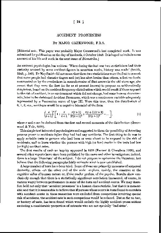
ACCIDENT PRONENESS BY MAJOR GREENWOOD, P.R.S. [Editorial note. This paper was probably Major Greenwood's last completed work. It was submitted for publication on the day of his death, 5October 1949. Itis hoped to include some account of his life and work in the next issue of Bimetrilca.] An eminent psychologist The first results of such an inquiry appeared in 1926 (Farmer & Chambers 1926), and several other reports This difficulty is not peculiar to the study of accident proneness. It is found in all attempts at a priori selection of persons suitable for occupations. But it is a serious difficulty because, until it is overcome, it means that we cannot by purely arithmetical methods discover the true frequency distribution of the variable we call accident proneness, because we only have the distribution of accidents. We can only guess. We know empirically that a very large proportion of accident distributions give some of the criteria a negative binomial, viz. the appropriate first and second moments of such a distribution. We know nothing more. E. M. Newbold (1927, pp. 504-5) in her classical memoir found in eleven instances that the proneness distribution was either in the type VI, or type I, area for ten cases while for one case it was in the 'impossible area', when the first four moments of the accident distributions were used. She justly remarks that, owing to the large probable errors of the higher moments and the fact that type I11 is at the dividing line of two areas, all one could say was that type I11was a reasonable choice. Readers of Biometrika do not need be told that because an aggregation of frequency distributions, made by summing the zeroes, the l's, the 2's, etc., of the separate distributions, give a negative binomial, the finding is no proof that proneness was responsible. We should necessarily reach a negative binomial if the items so aggregated were Poissons-unless, of course, they were identical Poissons (Pearson, 1917, p. 139). Some beginners have overlooked this. It may, perhaps, be worth noting that if the com- ponents aggregated-all 0's together, all 1's together, et~.-were Poissons, the variance of the resulting negative binomial will be smaller than it would have been if the several com- ponents were themselves negative binomials with the same means. There is an oddity about equation (1)as practically applied which has not been noticed. As the constants of the proneness distribution are deduced from those of the accident dis- tribution, they must vary from factory to factory if the external risk varies. But, by hypo- thesis, proneness is a character of the individual, a psycho-physiological property which exists whether he is subjected to the hazard of accidents or not. This did not affect the use of the method made by Greenwood & Yule, who assumed that in each factory the risk was constant, but it does make comparison of factory with factory difficult. Suppose then that we put the fundamental Poisson in the form e-kx(l+kx/l !+k2x2/2!+k3$/3 ! ...), (2) where k is constant for any one factory or department of a factory, but different for different factories or departments. Then our accident distribution will become cr/(c+k)'(l+kr/(c+k) 1!+k2r(r+ l)/(~+k)~2! (3) ...). At first sight, this is merely trivial; if we write in (2) y = kx, we simply have a straight Poisson in y, and if we write ck for c in (3) we are back to (1). But it does make some comparison between different sets of data possible and admits a process akin to the standardization of death-rates. Suppose we take an accident distribution, any accident distribution pro- vided it is effectively a negative binomial distribution with a mean m, and adopt this as the standard form, viz. assume its k to be unity. We take now another accident distribution having a different mean m' which again is a negative binomial. Now put k = m'/m and sub- stitute for the c of the standard form c/k = C.We shall have again a negative binomial having the required mean. Does this effectively graduate the experience? Trials on some of New- bold's data (Newbold, 1926) showed that this very naive plan did not give bad results, but they were not at all convincing because the range of means was narrow. She had, however, one pair of observations from the same factory, a manufactory of sweets, where the length of a k constant for any one factory department, but changing from department to depart- ment. But if we take as standard population any population with a greater mean and variance than the population to be standardized, then-provided the accident distribution of the latter is fairly well fitted by a negative binomial-we should expect the process to give us a fairly good fit. Common sense, however, tells us both selection of workers and differences of environmental risk are involved. After all, we know nothing more than the accident distri- butions given by samples, and not very large samples, of two populations; too much room for guessing remains even for those whose algebra is better than mine. Since the publication of Newbold's memoir, field workers have not bothered about a deter- - minist approach on these lines and have used Newbold's stochastic results. To these, with certain exceptions to be noted (see p. 28), little has been added; it has, however, been pointed out that the algebra would have been simplified by working with factorial instead of power moments. m Newbold defined statistical proneness as meaning that in unit population SfA,= 1, the 0 accidents happening to the subfrequency fA, will be distributed by a Poisson law with para- meter &, so that the 'accident universe' will be an aggregate of Poissons. What we have is a sample of persons from a universe so defined; from such a sample we can stochastically estimate the parameters of the 'universe'. By definition, the best available estimate of the mean X is the mean of accidents, A, and it is easy to see that if N (the number exposed to risk) is so large that N-1 does not differ appreciably from N, the best estimate of the variance of h is the variance of accidents less the mean. In the particular case leading to equation (1)this is obvious. The variance of the gamma function is r/c2, that of the accident distribution, r/c2+r/c. If Ai = A+ + ei,where s, is a sampling error and if hiand E, are not correlated, we have If some other variable, x,say the scoring of a person in a test, is correlated with his accident score, then These are the relations which have been used by field workers, whose object has been to reach a test, or battery of tests, which correlates highly with A. The difficulty of non-comparability of data collected under different environments of course remains. For instance, suppose correlations of test scores and,accidents vary signi- ficantly between different studies. Is that due to selection? Dr Irwin has pointed out to me how that question could be answered, if one had rather more adequate numerical data. But the variation of what I have called external risk remains. Any statistics of accidents must contain a number of events which have no connexion with the personal qualities of the exposed to risk. We may safely infer from what we already know that the proportion is not large, but it must vary with the occupation. I suppose a minute--and objective-record of every accident entered on the statistical statement might enable us to eliminate these, but it would be a statistician's paradise in which such information was available. Between 1927 and 1941 no important additions were made to the field-worker's statistical took, but at least two mathematical statisticians pointed out that a negative binomial REFERENCES CHAMBERS, E. G. (1941). J.R. Statist. Soc. Suppl. 7, 89, 95. FARMER, E. G. (1926). Rep. Industr. Fatig. Rcs. Bd, no. 38. E. & CHAMBERS, H.AI.S.0. FARMER,E. & CHAMBERS, E. G. (1939). Rep. Industr. HltA 12es. Bd, no. 84. GREENWOOD, M. (1941). J.R. Statist. Soc. Suppl. 7, 107. GREENWOOD, M. & YULE,G. U. (1920). J.R. Statist. Soc. 83,255. IRWIN,J.0.(1941). J.R. Statist. Soc. Suppl. 7, 101. NEWBOLD, E. M. (1926). Rep. Industr. Fatig. Res. Bd, no. 34. H.M.S.O. NEWBOLD, E. M. (1927). J.R. Statist. Soc. 83,255. PEARSON, K.(1917). Biometrika, 11, 139. SMITH,MAY(1943). An Introduction to Inrl~~trial Lond~r. Psychology. YULE,G. U. (1941). J.R. Statist. Soc. Suppl. 7, 91.