Comparing more than two means and figuring out which are different Analysis of Variance ANOVA Despite the name the procedures compares the means of two or more groups Null hypothesis is that the group means are ID: 243718
Download Presentation The PPT/PDF document "Analysis of Variance and Multiple Compar..." is the property of its rightful owner. Permission is granted to download and print the materials on this web site for personal, non-commercial use only, and to display it on your personal computer provided you do not modify the materials and that you retain all copyright notices contained in the materials. By downloading content from our website, you accept the terms of this agreement.
Slide1
Analysis of Variance and Multiple Comparisons
Comparing more than two means and figuring out which are differentSlide2
Analysis of Variance (ANOVA)
Despite the name, the procedures compares the means of two or more groups
Null hypothesis is that the group means are
all
equal
Widely used in experiments, it is less common in anthropologySlide3
ANOVA in Rcmdr
Statistics | Means | One-way ANOVA
Accept or change the model name
Select a group (only factors are listed here)
Select a response variable (only numeric variables are listed here)
Check
Pairwise
comparison of meansSlide4
> AnovaModel.1 <-
aov
(Area ~ Segment, data=Snodgrass)
> summary(AnovaModel.1)
Df
Sum Sq Mean Sq F value Pr(>F)
Segment 2 432327 216164 51.817 1.344e-15 ***
Residuals 88 367107 4172
---
Signif
. codes: 0 '***' 0.001 '**' 0.01 '*' 0.05 '.' 0.1 ' ' 1
>
numSummary
(
Snodgrass$Area
, groups=
Snodgrass$Segment
,
+ statistics=c("mean", "
sd
"))
mean
sd
n
1 317.3711 76.08797 38
2 166.7946 59.99526 28
3 192.7900 48.18188 25Slide5
Results
Since the ANOVA statistic is less than our critical value (.05), we reject the null hypothesis that the mean Areas of Segments 1 = 2 = 3
But we usually want to know more
Since we did not make predictions in advance our comparisons are post hocSlide6
Multiple Comparisons
To find out which means are different from each other we have to compare the various combinations: 1 with 2, 1 with 3, and 2 with 3
(we could also perform other comparisons such as 1 and 2 with 3 but they are rare in anthropologySlide7
More Kinds of Errors
Our statistical tests have focused on setting the Type I error rate at .05 – the
comparisonwise
error rate
But this error rate holds for a single test. If we do many tests, the chance that we will commit at least one Type 1 error will be higher – the
experimentwise
error rateSlide8
Calculating Errors
If the probability of a Type I error is .05, the probability of not making a Type I error is (1 - .05) = .95
The probability of not making a Type I error twice is .95
2
= .9025, three times - .95
3
= .8574, four times - .95
4
= .8145Slide9
Calculating Errors
The probability of making at least one Type I error is
Twice – (1 - .9025) = .0975
Thrice – (1 - .8574) = .1426
Four times – (1 - .8145) = .1855
The probability of making at least one Type I error increases with each additional testSlide10Slide11
curve((1-(1-.05)^x), 1, 50, 50,
yaxp
=c(0, .9, 9),
xaxp
=c(0, 50, 10),
xlab
="Number of Comparisons",
ylab
="Type I Error Rate",
las
=1,
main="
Experimentwise
Error Rate")
curve((1-(1-.01)^x), 1, 50, 50,
lty
=2, add=TRUE)
text(30, .92, expression(p == 1-(1-.05)^x), pos=4)
text(30, .37, expression(p == 1-(1-.01)^x), pos=4)
abline
(h=
seq
(.1, .9, .1), v=
seq
(0, 50, 5),
lty
=3,
col
="gray")
legend("
topleft
", c("
Comparisonwise
p = .05",
"
Comparisonwise
p = .01"),
lty
=c(1, 2),
bg
="white")Slide12
Multiple Comparisons
Multiple Comparisons procedures take
experimentwise
error into account when comparing the group means
There are a number of methods available, but we’ll stick with
Tukey’s
Honestly Significant Differences (aka
Tukey’s
range test)Slide13
Tukey’s HSD
One of the few multiple comparison tests that can adjust for different sample sizes among the groups
You requested this test in
Rcmdr
when you checked “
Pairwise
comparison of the means”Slide14
> .Pairs <-
glht
(AnovaModel.1,
linfct
=
mcp
(Segment = "
Tukey
"))
> summary(.Pairs) #
pairwise
tests
Simultaneous Tests for General Linear Hypotheses
Multiple Comparisons of Means:
Tukey
Contrasts
Fit:
aov
(formula = Area ~ Segment, data = Snodgrass)
Linear Hypotheses:
Estimate Std. Error t value Pr(>|t|)
2 - 1 == 0 -150.58 16.09 -9.361 <1e-04 ***
3 - 1 == 0 -124.58 16.63 -7.490 <1e-04 ***
3 - 2 == 0 26.00 17.77 1.463 0.313
---
Signif
. codes: 0 '***' 0.001 '**' 0.01 '*' 0.05 '.' 0.1 ' ' 1
(Adjusted p values reported -- single-step method)Slide15
>
confint
(.Pairs) # confidence intervals
Simultaneous Confidence Intervals
Multiple Comparisons of Means:
Tukey
Contrasts
Fit:
aov
(formula = Area ~ Segment, data = Snodgrass)
Quantile
= 2.383
95% family-wise confidence level
Linear Hypotheses:
Estimate
lwr
upr
2 - 1 == 0 -150.5764 -188.9093 -112.2435
3 - 1 == 0 -124.5811 -164.2161 -84.9460
3 - 2 == 0 25.9954 -16.3553 68.3460Slide16Slide17
NonParametric ANOVA
The non-parametric alternative to ANOVA is the
Kruskal
-Wallis Rank Sum Test
The null hypothesis is that the medians of the groups are equal
If the test is significant, a multiple comparison method is available to identify which groups are differentSlide18
Kruskal-Wallis in Rcmdr
Statistics | Nonparametric tests |
Kruskal
-Wallis test
Select a group (only factors are listed here)
Select a response variable (only numeric variables are listed here)Slide19
Multiple Comparisons
If there are significant differences the function
kruskalmc
()
in package
pgirmess
will tell you what groups are differentSlide20
>
kruskal.test
(Area ~ Segment, data=Snodgrass)
Kruskal
-Wallis rank sum test
data: Area by Segment
Kruskal
-Wallis chi-squared = 50.4427,
df
= 2, p-value = 1.113e-11
library(
pgirmess
)
>
kruskalmc
(Area ~ Segment, data=Snodgrass)
Multiple comparison test after
Kruskal
-Wallis
p.value
: 0.05
Comparisons
obs.dif critical.dif difference
1-2 43.125940 15.74873 TRUE
1-3 35.227368 16.28369 TRUE
2-3 7.898571 17.39936 FALSE