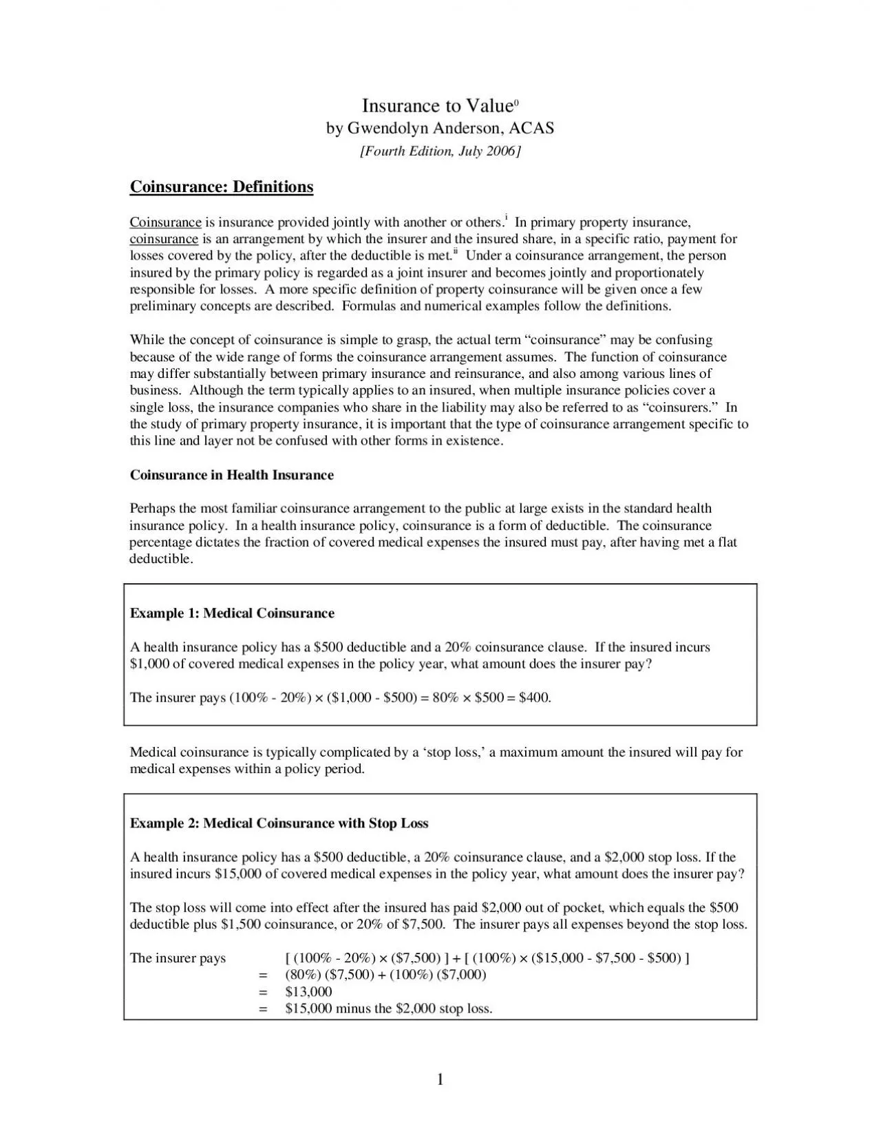
mplicated by a stop loss a maximum amount the insured will pay for - PDF document

mplicated by a ‘stop loss,’ a maximum amount the insured will pay for medical expenses within a policy period. Example 2: Medical Coinsurance with Stop Loss = (80%) ($7,500) + (100%) ($7,000) = $13,000 = $15,000 minus the $2,000 stop loss. The maximum coinsurance apportionment ratio is . The designated insurance (represented in the numerator of the coinsurance apportionment ratio) may be: the face amount of the policy requiring insurance, the total face amounts of the insuunder provisional reporting form policies, full insurance on the property values last reported is any policy provision that establishes a coinsurance arrangement. The coinsurance requirement is the least amount of insurance for which the coinsurance apportionment ratio will equal ing with the format apportionment ratio, the coinsurance requirement may be either (i) a stated sum, or (ii) a specified percentage of the value of the insured property. Under a provisional reporting form policy, the requirement may equal the true aggregate value of all property at the date of the latest report.

As stated previously, when the coinsurance requirement is met, the coinsurance clause will not reduce indemnity for is the amount by which a coinsurance requirement exceeds the carried insurance presently applicable to the coinsurance requirement. is the amount, greater than zero, by which an indemnity payment for a loss is is an insured that fails to meet a coinsurance requirement, and is thus exposed to possible coinsurance penalties. A coinsurer provides a higher level of ‘self-insurance’ than an insured that meets the coinsurance requirement. A loss ncoinsurer; according to the terms ofoviding protection up to the maximum deficient policy is paid, the insured bears a portion of the loss but as a coinsurer. An insured with less than full coverage may be entitled to the full face amount of the policy whapplies, and in that case, no coinsurance penalties are considered to exist. exists if property is insured to the exact extent assumed in the premium rate calculation. The rate calculation may assume that the average level of coverage is less than 100% of th

e value of the property means insurance to only if 100% coverage is assumed in the rate computation. Underinsurance is coverage less than that assumed, and overinsurance is coverage beyond that assumed. As the concept of insurance to value is so closely tied to the premium rate calculation, it will become clearer later in the paper once the appropriate equations have been derived. The following variables will be used to define simple coinsurance relationships: = the indemnity received by the insured for a loss = the dollar amount of the loss (after the flat deductible is met) = the face amount of insurance = the dollar value of the property = the coinsurance percentage may be insured under periodic reporting forms. These types of policies have no face amounts, but description and value of the covered property at each location and the amount and terms of specific insurance.Reports are typically made on a monthly basis. The standard coinsurance mechanism may be represented by a simple formula. The coinsurance clause establishing the most general coinsurance arran

gement provides that: = = F / cV ]. [Equation 5.a] subject to two constraints: I ≤ F [Equation 5.c] Equation 5.a dictates that losses are apportioned between the insurer and its insured according to the standard definition of coinsurance, such that the insurer pays a fraction of the insured loss equal to the coinsurance apportionment ratio. The first constraint is that the indemnity payments be limited to the loss amount. This constraint is due to the principle of indemnity , the concept that no insured should profit from any loss. It also follows mathematically from Equation 4 and the limitation of coinsurance apportionment ratio, [ ]: if the ratio were allowed to exceed one, the amount indemnified could exceed the loss amount; but the indemnity payment must never exceed the loss amount, ng to insure beyond the coinsurance requirement. The second constraint limits the indemnity payment to the which sets the overall limit on the amount of insurance payable on a single occurrence. Coinsurance PenaltiesBy definition, a policyholder is deemed a simply by holdin

g a policy with a deficiency to arise: a covered loss greater than zero must occur whamount greater than zero is payable beyond the flat deductible and any other restrictions on the policy: � 0 ; [Equation 6.a] (2) a coinsurance deficiency must exist on the policy insuring the loss, i.e. - the insured must fail to meet the coinsurance requirement, such that: ; andd (3) as no coinsurance penalty is said to exist if the indemnity is Equation 5.b), it follows that for a coinsurance penalty to exist, the indemnity payable must fall = = F / cV ] c By definition, the coinsurance penalty ceases to exist at the point where the indemnity payable equals the policy face. The loss amount corresponding to this indemnity payment may be fully derived as follows: = a L F [ F [ cV 7 Example 5: The Standard Coinsurance Clause Immediately before a fire breaks out, a property is valued at $500,000. The coinsurance requirement for the policy is 80% of the property value. The building suffers a covered loss of $450

,000. What is the indemnity payment on the loss, and what is the coinsurance penalty, if the insured carries a policy with (1) a $300,000 face value? (2) a $500,000 face value? (1) = ($450,000) × [ $300,000 ÷ (80%) × ($500,000) ] = ($450,000) × (0.75) = $337,500 but $300,000, the policy face amount. = $300,000 = the indemnity payment = $0 �= no coinsurance penalty exists (2) = ($450,000) × [ $500,000 ÷ (80%) × ($500,000) ] = ($450,000) × (1.25) = $562,500, but the coinsurance apportionment ratio can not exceed $450,000, the loss amount. = $450,000 = the indemnity payment = $450,000 - $450,000 = $0 �= no coinsurance penalty exists 25,00050,00075,000100,0000100,000200,000300,000400,000500,000 Loss Amount The coinsurance penalty for a given coinsurance requirement is an increasing function of the loss amount up to the policy face. For loss amounts greater than the policy face, the penalty is a decreasing function up to the coinsurance requirement. For losses equal to or exceeding the coinsurance requirem

ent, the full face value is paid and no coinsurance penalty exists. Graph 1 is based on the values in Example 4. Conditional and Unconditional Probability Distributions A probability distribution outcomes and for each outcome specifies a probability, the total value of which sum to , that is, to one hundred percent.A conditional probability distribution outcomes have been restriAn unconditional probability distribution has no restrictions on the set of outcomes. Conditional probability may be defined mathematically. Suppose that A and B are two sets of outcomes. The probability of B under the condition that A has happened, denoted by P(B | A) is given by: P(B | A) = P(A and B) [Equation 9] P(A) Generalized Loss-Severity Functions The following variables were previously defined: = the dollar amount of the loss (after the flat deductible is met) = the face amount of insurance = the dollar value of the property By assumption, each propertpolicy, and no policy insures more than one property. The unconditional probability of a loss of size insure

d, and, of these, suffer a loss greater than zero during a policy period, is the probability some nonzero loss during that period. The unconditional probability of a loss of denoted as p(given by: ) = () = [Equation 10] represents the frequency of loss, and the function s() represents the loss-severity distribution.Since few risks suffer a loss during a policy period, the integral of the unconditionalprobabilities from more than zero to is much less than , but over the range to loss”: [Equation 11]and it equals ounts for all possible outcomes.severity function s(conditionaloccurred, and excludes the outcome of ‘zero’ losses, that is, that no loss occurs. ) represent the percentage of all losses from a given peril that are of size may be represented either by the dollar amount of loss or its fraction of the property value. Then s() is the 11Coinsurance Illustrations This section demonstrates the function of coinsurance arrangement, as well as its short-comings, in solving or preventing problems of underinsurance.examine the inequities that could result if in

sureds were to purchase less insurance coverage than the amount assumed in the calculation of the pure premium rate. In the absence of coinsurance, policyholders might find they benefit by carrying low levels of insurance, and an insurer with a number of underinsured risks might not collect sufficient premium to meet its liabilities. The illustrations show how the coinsurance mechanism may be implemented to help the insurer collect adequate premiums, how coinsurance provides incentive for policyholders to maintain full coverage on insured property, and how coinsurance serves to promote equity among insureds. Following the illustrations, the case studyexample of the extreme troubles that can strike insurers and insureds alike when underinsurance is severe, far beyond remedy by Consider two people who own similar homes valued at $500,000 each. Anna insures her home for full to pay lower monthly premiums. Blanca knowingly retains the upper layer of risk for losses beyond $250,000. Neither policy contains any form of deductible. mnified equivalently for any fire loss under

$250,000. Blanca has paid a lower premium, but has received the same level of protection on any face. Is this arrangement “fair?” For simplicity, assume that the severity distribution is uniform, that all sizes of loss are equally likely. A loss above $250,000 is equally likely as a loss below $250,000. Assuming the insurer believes that all of its insureds are purchasing full coverage, it will charge Blanca exactly half the pure premium it charges and Blanca would receive the same indemnity payment equal to the loss amount; this case applies to losses of up to $250,000. In the other half of the instances, full amount of the loss while Blanca would receive her policy face of $250,000. Anna’s expected indemnity payment is equal to her expected loss of $250,000, while Blanca’s expected indemnity payment is $187,500. Note that this amount is 50% higher than half of Anna’s. While Blanca pays only half of the full-coverage premium, she can expect to be indemnified by more than half of the loss amount for any loss size short of a total loss. Blanca has selected less covera

ge but is clearly getting a better deal for the price. If these were the only two insureds, Anna’s premiums would subsidize some of Blanca’s exposure to loss. Anna would have clear incentive to lower Since the insurer has assumed in its premium rate d will maintain coverage equal to 100% of their property’s value, the insurer could remedy the situation by adding a coinsurance clause to the policy establishing a 100% coinsurance requirement. If such a requirement were added to the policy, Blanca’s coinsurance apportionment ratio would be 50%. She would coinsure half of every partial requirement which in this case is the total property value. On a fire loss of $200,000, Blanca would be indemnified $100,000, suffering a coinsurance penalty of $100,000. Such indemnity payments would balance with the premium payments. Similar results would follow even if all loss amounts were not equally likely. In half of the instances, Blanca receives the policy face average payment is uniformly distributed from $0 to $250,000. Blanca’s average indemnity payment is therefore ent is there

fore ()× ($250,000) + (0.50) × ($125,000)] = $187,500. 13 Case Study: The Oakland Firesiii,iv On October 20, 1991, a firestorm swept the hills of Oakl Francisco Bay. In the fires, 25 people were killed and 150 injured, and a total of 3,354 dwellings were destroyed at once with damages estimated at over $1.5 billion. In the aftermath, many homeowners were shocked to find their properties grossly underinsured. The Oakland fires were characterized by underinsurance so severe as to arouse panic surrounding the Claimants who had paid insurance premiums for years feared most of their losses - their homes, cars, and all of their possessions - would be irrecoverable. The policyholders of one insurance group estimated the cost of rebuilding their homes at $150 to $300 per square foot, but found their insurance would pay only $66 to $93 per square foot. Payments made on behalf of the forty insureds of another company fell short by an average of $130,000 per insured structure. In a survey of 27 insurance companies concerning 2,465 of the covered structures, 49% f

elt that the structures included in the survey had been underinsured by an average of $102,000. In a separate survey of 665 homeowners, 83% felt they were underinsured by an average of $194,000. Insurance companies said that under the law, it is the homeowner’s responsibility to make sure they have enough coverage. Many of the policyholders said that they had not understood the promise of “guaranteed replacement coverage” in their contract which had been denied. Appraisal methods used by some insurers to establish replacement cost, such as a method of appraising the structures room by room, were found to be te its were numerous. In the end, sting insurance companies $80 million. Two insurance groups received commendations from the California Department of Insurance. One of these, the California Casualty Group, made a decision early in the process to cover all policyholders to the full extent of their losses, regardless of the varying extents to which they were underinsured. The decision was based largely on the group’s claims philosophy, described by

Ed McKeon, Vice President of Corporate Relations: “Find a way to pay the claim, not California Casualty Group specializes in educator and public safety associations and does not insure “every third home on the street,” it felt an extra-contractual obligation to its insureds. At the time, California Casualty would not have expected its policyholders to be carrying enough insurance to recover from such an extreme situation. “Insurance appraisers aren’t expecting foundations to crumble and driveways to slide ure remains [following a fire].” There were drawbacks to the decision. McKeon felt that the California Casualty Group set a standard that the Department of Insurance used as a basis for measuring the performance of other companies not specializing in associations and not sharing the same claims philosophy, creating some tension within the local industry. Similar friction arose within the group, as some underinsured claimants in single family fires following the Oakland disaster expected similar treatment from the group. Clearly, it would not be feasible to

provide full coverage to underinsured policyholders under all circumstances. Since the Oakland fires, many improvements have been made both in coverage terms and in the tools and techniques of appraisal. Some policies contain a clause which, in the event of a total or near-total loss, allow the policyholder to be reimbursed by a proportional amount in excess of the face amount if they have maintained the required coverage level. Appraisals have become far more accurate so the face amount is not left entirely up to the insured to determine as might have been the case in the past. “Today, most underinsureds are people who have made improvements and upgrades or to tell us,” said McKeon. Large settlements emphasize the importance for insurance companies to monitor the level of insurance train employees, appraisers and agents to properly advise insureds, inform them of contract terms, take accurate measurements a 15 re similarly shaped, and basis for developing a premium rate schedule if this were the case. This assumption will not always be reasonable, and

other types of distortions may be introduced into such a model. numerous attributes. One variation straightforward to imagine is the physical size. Properties which are small in size are more prone to total and near total losses than large structures. For instance, imagine a small historic home in an upscale urban area which is appraised at an equivalent dollar value as a modern ranch house five times its size in a remote, low-cost rural area. While the two structures may be insured by policies with equivalent face values, both their loss frequencies and their size of loss distributions differ. The territory relativities applied in rating these policies will most likely account for the difference in frequencies; this may be due to the greater fire hazard in historic areas caused by faulty old wiring or the great spread in densely populated regions. Should both buildings incur fire damage, it is more likely that the small home will be damaged to a greater extent or completely destroyed than the large ranch house, simply because it is comprised of far less mater

ials taking less time to burn. Territory relativities applied as straight factors will generally not adjust for differences in the shape of loss distributions. It is not a common practice to separate small- versus large-sized properties in developing premium rates, but greater accuracy in rate making could A common practice is to separate properties into di property values. This practice could eliminate much of the distortion in combined distributions, whether losses are reflected in dollar amounts or as percentages of the property value. Such a division may even serve as a reasonable proxy to size, depending on how well territories delineate variations in cost levels and how territorial differences are addressed. "Small" properties"Large" properties Assume for simplicity the loss-severity distributions of all properties are similarly shaped, linear and downward sloping. It ispricing properties of any size. Scaling the losses, by representing each loss as a percentage of its property value, can eliminate this type of distortion if the loss distributions fo

r the individual properties are similarly shaped. The shape of among properties which are dissimilar in various ways including in their physical size, immediate su The homogeneity of insured properties dictates that the properties of a given class have the same relative frequency of loss, and the same loss size distributions, s(). In reality, these rate determinants for a given property are unknown. For example, a home with a fire hydrant directly in front of it may follow a different severity function than homes two and three blocks from the hydrant, yet all of the homes in this neighborhood may be deemed similar enough to group in the same class for rating purposes. To develop the rating model, it is assumed that the frequency and severity variables for the given property class are known and are not subject to changes due to dynamic influences (e.g. technological advances, changes in economic conditions, etc.). For the coinsurance mechanism to function accurately, it is necessary to be determinable and for coinsurance penalties to beand loss adjustment are assumed to b

e precise in order to arrive at presumably accurate pure premium rates. The complication of pro-ration among insurers can be eliminated from the model through a simple assumption. Assuming that the property is covered by one policy only, the estimation of the expected value of indemnity payments is greatly simplified. The model also ignores interest on pure premiums collected for the sake of simplicity. Pure premium is usually collected at the beginning of the policy period, or at quarterly or monthly intervals, while the loss payment would occur at the middle of the period on average. A greater degree of precision could be achieved by adding interest to the model, but this rating determinant does not benefit the study of coinsurance and therefore does not warrant the increased complexity. Although it will be assumed otherwise, it is definitely to incur more than one loss in a policy period. The model accounts for this by incorporating multiple lossethe frequency variable. The loss frequency is estimated by studying the total number of losses to many properties over

many policy periods. The relative frequency selected to represent the loss potential assumed for a single property is actually based on data that reflects multiple losses to a single property during a single policy period. The exclusion of multiple losses simplifies rate computation, avoiding the problem of double weight being given to multiple losses, an error to which the formula is prone, and ultimately avoiding an inflated redundant aggregate premiums. The following variables and notations were previously defined: = the dollar amount of the loss = the face amount of insurance = the dollar value of the property = the probability of any loss of whatever size greater than zero, to each insured property per policy period. s() = the percentage of losses exactly equaling , or the conditional probability of a loss of , given some loss greater than zero (L) = f) = the unconditional probability of a loss exactly equal to to The following variables and notations are now defined: = the pure premium charged each insured per policy period =

the pure premium rate per dollar of face amount per policy period ( can take on only discrete integer values, or: E) = [Equation 16.b] if the values of are continuous. The second element of an insurer’s expected indemnity payments, the limit times the probability of losses multiplied by the difference between one and the percentage of losses not E) = = 1 – Σ s(L)] [Equation 17.a] L 1 – Σ s(L) ] can take only discrete integer values, or: E) = = 1 – ∫ s(L)dL] [Equation 17.b] 1 – ∫ s(L) dL]

is a continuous variable. Note that Equation 17 simplifies to Combining the above expressions, the total of an insurer’s expected indemnity payments under one policy during one policy period can be expressed as: E EΣ s(L)]) [Equation 18.a] =1 Third, if the insured’s loss and the insurer’s liability are limited only by the property value, the numerator on the right-hand side of Equation 19 is the expected value of losses from zero to full value. The second, bracketed, element in the numerator of Equation 18 Automobile physical damage insurance is a common example. L=V V R 0 [Equation 21.a] [Equation 21.b] A variation of this case is a policy with an agreed amount endorsement. Since, under an agreed amount y value determined by anace can be presumed impossible. each $100 of an agreed amount of insurance,

L=F R /100 [Equation 22.a] [Equation 22.b]policy face, which may be less than where property values and amounts of insurance are definite and separable, that entails the topic of insurance to value. A special problem arises whpremium rate can be appropriate only if each insured med in the premium rate lution to the problem of insureds selecting policy faces different from that assumed in the premium rate computation. exists if property is insured to the exact extent, either dollar amount or percentage of value, as assumed in the premium rate calculation. The rate calculation may assume that the average level of coverage is less than 100% of the value of the property means insurance to only if 100% coverage is assumed in the rate computation. The term “value” refers to the value of the property, on the same basis used in indemnifying losses; that basis is usually actual cash value. The replacement value of property is equal to the amount it would cost to fully

repair or replace the property if it must be The actual cash value (ACV) is equal to the “…replacemenenubtracting an amount that reflects depreciation. …The actual cash value of an item can be depressingly small after only a brief period of ownership.” If the premium rate is based on 80 percent insurance to replacement cost, neither coverage to 90 percent of replacement cost constitutes “insurance to than replacement cost; in the second instance, the property is overinsured relative to the insurance to value relationship assumed in the premium rate. her property will be an amount quite a bit greater than half of the full coverage pure premium. Although the illustrations assumed a uniform loss size distribution, the equitable premium for the significantly underinsured the full-coverage premium than the proportion of the property value insured. Premium gradation may be viewed as an alternative to coinsurance; however, such a method requires the red property and determine when and by how much it is changing. The pure premium rate was derived using both discrete and con

tinuous notations to represent loss amounts. Since every currency has a smallest monetary unit, such as the in the United States, the continuous case is not technically valid. Since fractional cents are not possible loss amounts, the continuity of the loss severity distribution is broken at the regular small increments of the cent. However, this technicality does tion since the smallest monetary unit is generally very small in relation to typical loss sizes. In light of penny increments, the shape of the size of loss distribution can be expected to at least approach the continuous case. A greater hindrance to achieving an ncy for loss amounts to cluster. Insurers and insureds alike tend to settle for and to prefer round values such as $10,000 instead of $9,765.24 or $10,014.12; or $50,000 as opposed to $49,983.87 or $50,374.28. the loss variable which are difficult to describe in the discrete notation. One example is the mathematical derivation of the change of rate with face. The assumption that continuous variable will be assumed in this instance whdis

crete notation. Change of Rate with FaceWhenever losses less than the pure premium rate should fall as the policy face increases, either absolutely or relative to value. This property holds regardless of the shape of the size of loss distribution, and even if large losses predominate. In the words of the Merritt Committee ReportThe principle that the rate falls as the ratio of insurance to value increases relatively more frequent than small ones. e first derivative of the premium rate = = ∫ s(L) dL] )} [Equation 19.b] the derivative is: F dR = F s(F) + (1 – ∫ s(L)dL ) + F (– s(F)) ] F F – ∫ L s(L) dL + F ( 1 – ∫ s(L)dL ) ] 0 0 (continued) V 200,000 = 180 [ 0 = 0.18 ( - 5.0 10 -11 3 + 10 -5 3 2 = ( - 3.0 = - 24,000 + 36,000 = $12,000 (3) R

R∫ s(L) dL] }) / 100) RR∫ ( -5.0 × 10 -11 ) L + (10 -5 )dL] }) ( / 100) R / 3 + (10 / 2] + { 10 -11 2/2 - (10 -5 ] }) ( / 100) R / 3 + (10 / 2] + [1 - / 2 + (10 ] ) R18] = (1.5 10 -10 2 - ( 9.0 10 -5 10 1 ) 18 = $ 10.50 +18 = $ 10.20 = (1.5 dR/dF = ( 3.0 dR/d(100,000) = ( 3.0 ) = 6.0 (5,000)(6.0 ) = -$0.30 $10.50 - $10.20 = -$0.30 (continued) (continued) (continued) (1) Graph the two functions on the interval 0 200,000, to confirm graphically that small losses predominate for s(L) while large losses predominate for v(L). (2) Show mathematically that s(L) is a decreasing function of L and v(L) is an increasing function of L. (3) Find the equation for the pure premium rate per $100 of insurance, , ba

sed on the loss size function, v( (4) Graph the pure premium rates for s(L) and v(L) using the equations found in Part (3) of Example 8 and Part (3) of this example. (5) Find the second derivatives of the pure premium rates for s(L) and v(L), and explain what the second derivatives imply about the shape of the pure premium rate curves. 0.00000.00010.00020.00030.00040.00050.00060.00070.00080.00090.0010$10,000$20,000$30,000$40,000$50,000$60,000$70,000$80,000$90,000$100,000$110,000$120,000$130,000$140,000$150,000$160,000$170,000$180,000$190,000$200,000Percent of Losses Large Losses Predominate Small Losses Predominate s(L) = (-5.0 * 10^-11) L + 10^-5 v(L) = (5.0 * 10^-11) L (2) Find the first derivatives of the two linear functions: s ' ( s(L) is a decreasing function of L v ' () = 5.0 � 0 v(L) is an increasing function of L (3) RR∫ v(L) dL] }) / 100) (continued) (continued) (continued) R[v(L)] was found in Part (3) of this example: R[v(L)] = ( - 1.5 dR[v(L)] /dF = ( - 3.0 R[v(L)] /dF = ( - 3

.0 R[v(L)] is concave down. R[s(L)] /dF is positive, R[s(L)] is concave up and rates are decreasing at a decreasing rate. R[v(L)] /dF is negative, R[v(L)] is concave down and Pure Premium Coinsurance Rates As stated earlier, a particular pricing problem arisespremium rates can be appropriate only if each insured chooses the policy face assumed in the rate are computed on the assumption coinsurance requirement. If the policy face is less thssumed, the coinsurance mechanism will balance pure premiums and expected indemnity payments. While the coinsurance mechanism can ensure balance below the level assumed in that which is assumed. Since proper pure premium rates vary inversely with coinsurance requirements, the insured who selects coverage exceeding that requirement will be pae policy will never indemnify beyond property value. A coinsurance rate for full coverage must be made available to ensure equity to all insureds. Note that the insured may collect total indemnity payments greater than the full property value when “additional coverages,” such as debris remov

al, apply. Such coverages may be included in a homeowner’s Under a percentage of value coinsura, from those percentages made available. Recall that the coinsurance requirement, , is given by: C = ; Since the pure premium coinsurance rate relativities are determined by the distribution of losses as percentages of value, any property value, tion. Because the assumed policy , the premium rate equations, from Equations 19.a and 19.b, become: L=C L=CCΣ s(L) dL] }) [Equation 24.a] F is discrete, The question is whether or not gross premium rates decline in the same manner as pure premium rates, as outlined in Table I? Rating formulas will often represent loadings as a constant percentage of pure premium. Alternatively, expense loadings may also commonly be fixed in amount. If all loadings are a constant percentage of the pure premium rate, gross rates will be a constant multiple of pure rates; the gross rates will have the same red. Loadings that are a fixed amount represent a decreasing percentage of the premium rate as the p

oWhen small losses outnumber large ones, as in case (a) of Table I, fixed loadings will cause gross rates to still decrease at a decreasing rate, although faster than the underlying pure rates. When large losses outnumber small ones, as in case (c), whether the rate of decrease in gross rates is increasing or decreasing will depend on both the skewness of the size of loss distribution and the amount of the fixed loadings.Fixed loadings will more certainly impact case (b), where loss sizes are uniform, causing the gross rates to decrease at a In most size of loss distributions, small losses - losses that are small percentages of value - outnumber large ones. This property will lead to both pure and gross coinsurance rates which decrease by decreasing amounts as the coinsurance requirement increases over equally-sized increments. This will be true whether loadings are variable or fixed.A premium reversal incremental premium rates is more insurance is less than the cost of less insurance.in the gross premium rate ease in the policy face, a premium revepremium reversal will le

ad to a negative marginal revenueng that the marginal cost of that additional insurance is also negative. As this can not be the case, most premium reversals are actuarially incorrect and should be avoided. There are a few normal circumstances under which minor premium reversals may occur. In the instance boundaries of the bands. For example, if coinsurance percentages are grouped in bands at 10 percent intervals, a premium reversal could exist between 89 and 90 percent of coverage, such that the policy would cost less at 90 percent coinsurance than at 89 percent coinsurance. Even so, no reversals should be within the range from 80 to As noted earlier, the coinsurance mechanism balances premium rates with expected indemnity payments so that rates will be equitable and just adequate. While the coinsurance mechanism allows for rate adequacy below the level assumed in the rates, such a result is not achieved that which is assumed.For coinsurance to function as intended, the insurer must provide a full range of coinsurance requirements and credits. Each coinsurance requi

rement should specify a separate rate which dictates the appropriatecredit. The coinsurance requirements should be offered at small intervals to the greatest extent practical. A coinsurance clause should be attached to even the smallest of policies to create a balance of expected indemnity and pure premium. Insurance to value exists if property is insured to the exact extent assumed in the premium rate calculation. Maintaining insurance to value defines the goal of maintaining coverage among insureds at a level equal to that assumed within the actuarial premium rate calculations. Endnotes: The source of the core definitions and equations used in this paper is Insurance to Value , by George L. Head, CPCU, CLU, published by the S. S. Huebner Foundation for Insurance Education © 1971. Source: The Random House Dictionary of the ERandom House, Inc. Source: www.insure.com Source: The Oakland Tribune, April 1, 1992, page A-3, and April 2, 1992, page A-1, and June 11, 1992, Source: Interview with Ed McKeon, Vice President of Corporate Relations, California Casualty Group, Ma