/
259 Lecture 15 Introduction to MATLAB 259 Lecture 15 Introduction to MATLAB

259 Lecture 15 Introduction to MATLAB - PowerPoint Presentation

tatyana-admore
tatyana-admore . @tatyana-admore
Follow
369 views
Uploaded On 2018-03-14

259 Lecture 15 Introduction to MATLAB - PPT Presentation

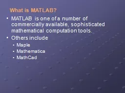
2 What is MATLAB MATLAB which stands for MATrix LABoratory is a highperformance language for technical computing It integrates computation visualization and programming in an easytouse environment where problems and solutions are expressed in familiar mathematical notation ID: 650355

matrix matlab octave command matlab matrix command octave file plot commands type array window inv function functions matrices colon

Share:

Link:

Embed:

Download Presentation from below link

Download Presentation The PPT/PDF document "259 Lecture 15 Introduction to MATLAB" is the property of its rightful owner. Permission is granted to download and print the materials on this web site for personal, non-commercial use only, and to display it on your personal computer provided you do not modify the materials and that you retain all copyright notices contained in the materials. By downloading content from our website, you accept the terms of this agreement.


Presentation Transcript

Slide1

259 Lecture 15

Introduction to MATLABSlide2

2

What is MATLAB?

MATLAB, which stands for “MATrix LABoratory” is a high-performance language for technical computing.

It integrates computation, visualization, and programming in an easy-to-use environment where problems and solutions are expressed in familiar mathematical notation.

Typical uses include:

Math and computation

Algorithm development

Data acquisition

Modeling, simulation, and prototyping

Data analysis, exploration, and visualization

Scientific and engineering graphics

Application development, including graphical user interface buildingSlide3

3

What is MATLAB?

MATLAB is an interactive system whose basic data element is an array that does not require dimensioning.

In many university environments, it is the standard instructional tool for introductory and advanced courses in mathematics, engineering, and science.

In industry, MATLAB is the tool of choice for high-productivity research, development, and analysis. Slide4

4

What is MATLAB?

MATLAB features a family of add-on application-specific solutions called

toolboxes

, which allow you to learn and apply specialized technology.

Toolboxes are comprehensive collections of MATLAB functions (M-files) that extend the MATLAB environment to solve particular classes of problems.

Areas in which toolboxes are available include signal processing, control systems, neural networks, fuzzy logic, wavelets, simulation, and many others.Slide5

5

The MATLAB System

The MATLAB system consists of these main parts:

Desktop Tools and Development Environment

The MATLAB Mathematical Function Library

The MATLAB Language (syntax)

Graphics

The MATLAB External Interfaces/Application Programming Interface (used to design software)Slide6

Octave – A Free MATLAB Clone

One of the “drawbacks” to MATLAB is that it is very

expensive (~$500

for an academic license).

One possible alternative to MATLAB is OCTAVE, which is a

free

clone of MATLAB (i.e. Octave mimics the functionality of MATLAB, often in the exact same way).

For more information on Octave (technically GNU Octave), see:

Octave downloads from Source Forge (both Windows and Mac OS X installers can be found here:

http://octave.sourceforge.net/

Octave Homepage:

http://www.gnu.org/software/octave/

6Slide7

7

MATLAB Desktop

Enter Commands here

in the Command Window

Current Directory

Window

Command History

WindowSlide8

Octave (CLI) – “Old Interface”

8Slide9

Octave (GUI) – “New Interface”

9Slide10

10

Calling MATLAB Help

To call Help in MATLAB, either click on the MATLAB Help link, or type “helpdesk” in the Command Window.

Octave does NOT have a built-in help file, so “helpdesk” doesn’t apply!

Notice that the Command History window keeps track of all of the commands you type!Slide11

11

Ending a MATLAB Session

To end a MATLAB session, type “exit” or “quit”.Slide12

12

MATLAB Basics

If you forget how to use a command, but can remember the command name, such as “plot”, type “help plot”.

A description of the command, along with syntax, options, related commands, and examples will appear!Slide13

13

MATLAB Basics

In MATLAB, another way to get information about a command is via “doc”, which gives more detailed information than “help”.

Try “doc plot

”.Slide14

14

MATLAB Basics

Many MATLAB functions are created from M-files, which are programs that contain a set of commands.

These commands are run in order to implement the function.

To see the contents of an m-file, use the “type” command.

This command does not work as well in Octave!

Try “type

linspace

”.Slide15

15

MATLAB Basics

To re-enter a command, use the up or down arrow, or type the first few letters of the command, and hit return!

To clear out your Command Window, use “

clc

”.

Commands in the Command History can be re-entered by double-clicking on them!

The Octave GUI must be on for this to work!Slide16

16

Entering Matrices

Matrices are the basic “building blocks” of MATLAB - essentially everything MATLAB does is based on calculations involving a matrix.

The most basic way to enter a matrix is by typing in the entries, inside square brackets, with row entries separated by spaces and new rows designated by semicolons.

Try entering these!Slide17

17

The Colon Operator

Another way to enter a matrix is via the colon, which is used to define increments within a vector.

Try each of the following:

x = [1:5]

y = [1:0.1:5]

z = [0:pi/4:2*pi]Slide18

18

The Colon Operator

We can “pull out” parts of a matrix with the colon!

Try each of the following:

A(2,:) is row 2 of matrix A.

A(:,3) is column 3 of matrix A.

B(1:2:3,:) is rows 1 and 3 of matrix B.Slide19

19

The Colon Operator

A(2,:) = [] removes the second row from A.

To insert the row back in, we can

concatenate

matrices via

A = [A(1,:); 0 -1 6; A(2,:)].

Try w = [x x].

For more information on the colon operator, type “help colon”.Slide20

20

Matrix Operations

To re-display matrix A, type “A”.

Matrix Operations:

Addition: +

Subtraction: -

Matrix Multiplication: *

Matrix Power: ^

Transpose – i.e. switch columns and rows (conjugate transpose in the complex case): ’

To transpose a matrix with complex entries, use .’

Inverse of a square matrix A: inv(A).

Matrix Left Division: \ (usage A\B = inv(A)*B)

Matrix Right Division: / (usage A/B = A*inv(B))

Example 1: Try each of the following!

A

B

A+A

A-A

A+B

A*B

B*A

inv(A)

A*inv(A)

A/A

A\A

A\B

inv(A)*B

A^3

A*A*A

A’

A(1,1) = 2+i

A’

A.’Slide21

21

Matrix Operations - Example 1 (cont.)Slide22

22

Array Operations

Scalar Multiplication: k*A with k a scalar.

“Normal” arithmetic works as expected with the usual order of operations – each number is a 1 x 1 matrix.

Array Multiplication, i.e. entry-wise multiplication of matrices of the same size: A.*B

Array Division, i.e. entry-wise division of matrices of the same size: A./B

Array Exponentiation, i.e. entry-wise exponentiation of matrices of the same size: A.^B

Example 2: Try each of the following!

A(1,1)=1

C = 5*A

C(:,1) = [1 1 1]

A.*C

A./C

A.*B

A.^C

A.*inv(A)

A.^3

1+2/3*4^7Slide23

23

Array Operations – Example 2 (cont.)Slide24

24

Special Matrices and Matrix Functions

“eye(n)” gives an n x n identity matrix

“zeros(m,n)” gives an m x n matrix of 0’s.

“ones(m,n)” gives an m x n matrix of 1’s.

“det(A)” computes the determinant of an n x n matrix A. (Recall that for A to be invertible, det(A)

0 must hold!)

To clear matrix A out of the Workspace, use “clear A”. To clear ALL variables out of the Workspace, use “clear all”.Slide25

25

Linear Systems of Equations

MATLAB can be used to solve systems of linear equations.

Example 3: Solve the system

x + 2y = 1

3x + 4y = -1

Solution: This system can be written in matrix form AX=b with:Slide26

26

Linear Systems of Equations

Example 3 (cont.)

Check if

det

(A)

0.

If so, then X = inv(A)*b will follow!Slide27

27

Making a Table of Values for a Function

MATLAB can be used to evaluate functions at input values entered as a vector!

For multiplication, division, and powers, use the array versions of these operators.

Example 4: Try the following commands to make a table of values of the function y = (x*sin(x

2

)-4)/(x+1).

x = [1:0.5:5]; % The ; suppresses output to the screen!

y = (x.*sin(x.^2)-4)./(x+1); % Array operators used here.

[x; y] % Concatenate the two vectors.

[x; y]’ % Transpose the matrix with x in column 1 and y in column 2 to get our table!Slide28

Creating an M-file

One of the most powerful features of MATLAB is the M-file, which is a file containing a set of commands that can be executed by MATLAB.

M-files syntax: *.m

These can be created as a text file and saved as an M-file.

To call the editor to make an M-file, type “edit”.

M-files can also be made from within MATLAB via pull-down menus File->New-

>Script

or by highlighting the commands in the Command History window.

In the Octave GUI, choose File->New

Script.

Create an M-file that contains the commands used to make the table in Example 4 above!

Save it on the Desktop as example4.m

28Slide29

29

MATLAB’s Path and Running an M-file

To run the M-file we created, we need to put the directory containing the file in MATLAB’s path.

To do this, type “

addpath

‘DIRECTORY’ ”,

where the ‘DIRECTORY’ is where the file is located, for example, a command like this should be used: “

addpath

‘C:\Users\MAK\Desktop’”

In MATLAB, this can also be done via the pull-down menus File->Set Path.

To run the set of commands, type the name of the M-file in the Command Window!Slide30

30

The Plot Command

MATLAB’s “plot” command is used to draw graphs of functions.

This is done by plotting (x, y) ordered pairs on a coordinate plane.

To plot the table created above, use the command “plot(x,y)”.

Notice that the graph we get is very jagged – to smooth it out, add more x-values and corresponding y-values to the vectors x and y!Slide31

31

The Plot Command

To the right is the same graph as above, with the commands:

x = [1:0.05:5];

y = (x.*sin(x.^2)-4)./(x+1);

plot

(

x,y

)

To

add

a

title

,

axes

labels

, and a

grid

to

the

graph

, use

the

title

”, “

xlabel

”, “

ylabel

”, and “

grid

commands

!

title

(‘y = f(x)’)

xlabel

(‘x’)

ylabel

(‘y’)

grid

on

Try

these

,

then

put

them

into

your

example4 M-

file

.

Try

plotting

y = x*

cos

(x)

on

the

interval

[-

,3

].Slide32

32

Plotting More Than One Function

To plot more than one function on the same graph, use the plot command with the sets of input and output variables listed in order: plot(x,y,x1,y1).

Colors and plot styles can also be specified – to see a complete list of the available options, type “help plot” or “doc plot”.

Here is how to plot the functions f(x) = x^2 and f’(x) = 2x on the same graph!

x = [-1:0.1:2];

y = x.*x;

y1 = 2*x;

plot(x,y,’ro’,x,y1,’b-’)

title(‘y = f(x) and y = f’’(x)’)

xlabel

(‘x’)

ylabel

(‘y’)

legend(’y=x^2’,’y’’=2x’)Slide33

33

Piecewise Defined Functions

In order to plot a piecewise defined function, we concatenate the separate pieces.

x1 = [-2:0.1:0];

y1 = x1.^2 + 1;

x2 = [0:0.1:2];

y2 = sin(x2) +1;

x = [x1 x2];

y = [y1 y2];

plot(

x,y,’g

’)

xlabel

(‘x’)

ylabel

(‘y’)

title(’f(x)=x^2, if x is in [-2,0]; sin(x) + 1, if x is in (0,2]’)Slide34

34

References

Using MATLAB in Calculus by Gary Jenson

MATLAB Help Files – Getting Started

MATLAB Tutorial from the University of Utah at

http://www.math.utah.edu/lab/ms/matlab/matlab.html

Octave

http://octave.sourceforge.net/

http://www.gnu.org/software/octave/