PDF-RESEARCH ARTICLES CURRENT SCIENCE, VOL. 91, NO. 3, 10 AUGUST 2006 296

Author : tatyana-admore | Published Date : 2015-08-01

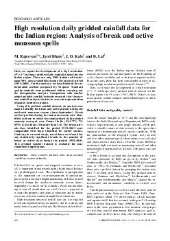
For correspondence email rajeevanimdpunegovin High resolution daily gridded rainfall data for the Indian region Analysis of break and active monsoon spells M Rajeevan1

Presentation Embed Code

<iframe width="560" height="315" src="https://www.docslides.com/embed/98056" frameborder="0" allowfullscreen></iframe>

Download Presentation

Download Presentation The PPT/PDF document "RESEARCH ARTICLES CURRENT SCIENCE, VOL...." is the property of its rightful owner. Permission is granted to download and print the materials on this website for personal, non-commercial use only, and to display it on your personal computer provided you do not modify the materials and that you retain all copyright notices contained in the materials. By downloading content from our website, you accept the terms of this agreement.

RESEARCH ARTICLES CURRENT SCIENCE, VOL. 91, NO. 3, 10 AUGUST 2006 296: Transcript

Download Document

Here is the link to download the presentation.
"RESEARCH ARTICLES CURRENT SCIENCE, VOL. 91, NO. 3, 10 AUGUST 2006 296"The content belongs to its owner. You may download and print it for personal use, without modification, and keep all copyright notices. By downloading, you agree to these terms.