PDF-An example of state feedback for an unstable and uncontrollable but stabilizable system

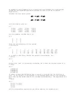
Consider the state space system with the A matrix given by a 65000 05000 65000 65000 05000 55000 55000 55000 05000 05000 05000 65000 05000 05000 55000 05000 For this example consider when B is b1 0 1 0 2 1 2 3 4 3 3 2 3 Check the controllability o. 1 Introduction to Eigenvalues Linear equations come from steady state problems Eigenvalues have their greatest importance in dynamic problems The solution of dt is changing with time growing or decaying or oscillating We cant 64257nd it by eliminat De64257nition 2 Computation and Properties 3 Chains brPage 3br Generalized Eigenvectors Math 240 De64257nition Computation and Properties Chains Motivation Defective matrices cannot be diagonalized because they do not possess enough eigenvectors to Reservation points have no other relationship with or com parison to vacation points and are established for convenience of reference only Reservation points are per person based on double occupancy and apply to 1 st and 2 nd passenger Ranges shown 1 Eigenvalues and the Characteristic Equation Given a matrix if 611 where is a scalar and is a nonzero vector is called an eigenvalue of and an eigenvector It is important here that an eigenvector should be a nonzero vector For the zero vector ace decdadcd good pe ni worthes, but mon ycan not moue, I keepe a fayer, but 8 good pe ni worthes but mon ycan not moue, Ikeepe a fayer but good pe ni worthes, but mon ycan not moue, Ikeep a fayer, bu KarlineSoetaert3example(image3D)example(contour3D)example(colkey)example(jet.col)example(perspbox)example(mesh)example(trans3D)example(plot.plist)example(ImageOcean)example(Oxsat)2.Functionsimage2Dand Review of properties of vibration and buckling modes. What is nice about them?. Sensitivities of eigenvalues are really cheap! . Sensitivities of . eigevectors. . . Why bother getting them? . Think of where you want your car to have the least vibrations. . can. be . interpreted. as a file of data. A . matrix. . is. a . collection. of . vectors. and . can. be . interpreted. as a data . base. The. red . matrix. . contain. . three. . column. Control . Systems. STATE FEEDBACK CONTROLLER DESIGN. Design . via. . Pole. . Placement. Design . via. . Pole. . Placement. Open . loop. . control. . system. Design . via. . Pole. . Placement. EIGEN … THINGS. (values, vectors, spaces … ). CONVENTION: . From now on, unless otherwise spec-. ified. , all matrices shall be square, i.e. . . . Another, less simple example:. . What are these . Bamshad Mobasher. DePaul University. Principal Component Analysis. PCA is a widely used data . compression and dimensionality reduction technique. PCA takes a data matrix, . A. , of . n. objects by . Prepared by Vince Zaccone. For Campus Learning Assistance Services at UCSB. Prepared by Vince Zaccone. For Campus Learning Assistance Services at UCSB. Consider the equation . , where A is an . nxn. MAT 275. A . linear system . is two or more linear equations in two or more variables taken together.. For example, . is a system of two linear equations in two variables.. A . solution of a system . Mark Hasegawa-Johnson. 9/12/2017. Content. Linear transforms. Eigenvectors. Eigenvalues. Symmetric matrices. Symmetric positive definite matrices. Covariance matrices. Principal components. Linear Transforms.