PDF-The Macroeconomics of HappinessRafael Di TellaHarvard Business SchoolR

Author : trish-goza | Published Date : 2017-02-05

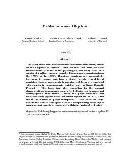
Corresponding author Rafael Di Tella Morgan Hall Soldiers Field Boston MA 02163 USA Forhelpful discussions we thank George Akerlof Fernando Alvarez Danny Blanchflower

Presentation Embed Code

Download Presentation

Download Presentation The PPT/PDF document "The Macroeconomics of HappinessRafael Di..." is the property of its rightful owner. Permission is granted to download and print the materials on this website for personal, non-commercial use only, and to display it on your personal computer provided you do not modify the materials and that you retain all copyright notices contained in the materials. By downloading content from our website, you accept the terms of this agreement.

The Macroeconomics of HappinessRafael Di TellaHarvard Business SchoolR: Transcript

Corresponding author Rafael Di Tella Morgan Hall Soldiers Field Boston MA 02163 USA Forhelpful discussions we thank George Akerlof Fernando Alvarez Danny Blanchflower Andrew Clark BenFri. Taggert J. Brooks. Module 02. Introduction to Macroeconomics. The Business Cycle. The . business cycle. is the short-run alternation between economic downturns and economic upturns. . US Business cycle dates from the NBER. FCS 3450. Spring 2015. Unit 1. Examples:. 1. Why do some couples choose to have three children while others elect to have none?. 2. Why do some families carry life insurance while others do not?. 3. Why do some families save to purchase major appliances while others buy them on credit?. Steve Keen. University of Western Sydney. Debunking Economics. www.debtdeflation.com/blogs. www.debunkingeconomics.com. Macroeconomics . Before . the Crisis: Triumphalism. “Macroeconomics . was born as a distinct field in the 1940's, as a part of the intellectual response to the Great . Forrest Stegelin. Agricultural & Applied Economics. University of Georgia. What is a “dashboard”?. In management information systems, a dashboard is . “an easy to read, often single page, real-time user interface, showing a graphical presentation of the current status (snapshot) and historic trends of an organization’s key performance indicators to enable instantaneous and informed decisions to be made at a glance.”. Module 35. What You Will Learn in this Module. Explain why . classical macroeconomics wasn’t adequate for the problems posed by the Great Depression. Discuss how . Keynes and the experience of the Great Depression legitimized . Junhui. Qian. Intermediate Macroeconomics. Content. Overview. GDP. Expenditure. Income. Inflation. CPI. GDP Deflator. Unemployment. Intermediate Macroeconomics. The importance of data. Sherlock Holmes: . La gamme de thé MORPHEE vise toute générations recherchant le sommeil paisible tant désiré et non procuré par tout types de médicaments. Essentiellement composé de feuille de morphine, ce thé vous assurera d’un rétablissement digne d’un voyage sur . Merin. Joy. Ph.D. Scholar in Economics, Government College . Kottayam. , . joy.mmerin@gmail.com. T. .M Jacob Memorial Government College, . Manimalakunnu. , . Koothattukulam. National Conference on Recent Macroeconomic Developments in India: Issues, Challenges and Remedies – 6-7, December-2017. PB 202 . MACROECONOMICS. Continuous Assessment . CA. Total. . Chapter. %. Quiz . Minimum. 3. Chapter. 1, 6, 7. 20. Test . Minimum 1. Chapter 1-4. 20. Tutorial . Minimum 2. Chapter 2&3. 20. Case study . 4 th H en June 23 rd to 24 th 2 01 8 On June 23 rd and 24 th 2018 , the Center for Financial Development and Stability (CFDS) at Henan University and the International Network for Economic Research for students attending the NU Bound Program These courses are for the Spring 2022 semesterfourof the following courses with the NU Bound England Program Calculus for Business MATH 1231 Calculus for MATCHES THE LATEST EXAM!Let us supplement your AP classroom experience with this easy-to-follow study guide!The immensely popular 5 Steps to a 5: AP Macroeconomics guide has been updated for the 2021-22 school year and now contains: 3 full-length practice exams (available in the book and online) that reflect the latest examAccess to a robust online platformComprehensive overview of the AP Macroeconomics exam formatHundreds of practice exercises with thorough answer explanationsReview material and proven strategies specific to each section of the testA self-guided study plan including flashcards, games, and more online Chapter 1 of . Macroeconomics. , 10. th. edition, by N. Gregory . Mankiw. ECO62. . Udayan. Roy. What Macroeconomists Study. Why are some countries rich and others poor?. Why have some countries’ incomes grown rapidly over the past decade while others have stagnated?. Booking business class flights has never been easier than with BuyBusinessClass. Their user-friendly platform allows you to browse through a wide range of options, view details of various airlines, and compare prices effortlessly.

Download Document

Here is the link to download the presentation.
"The Macroeconomics of HappinessRafael Di TellaHarvard Business SchoolR"The content belongs to its owner. You may download and print it for personal use, without modification, and keep all copyright notices. By downloading, you agree to these terms.