
1 State-Level Transportation Repricing to Reduce
T
Published · 13 slides · 0 views
1 / 1
Description
1 State-Level Transportation Repricing to Reduce Congestion Improve Affordability Presented by: Allen Greenberg, FHWA Office of Operations Federal Highway Administration Office of Operations 2025 Modeling Mobility Conference Minneapolis,
Related Topics
Share
Embed code
Download this presentation From Below
"1 State-Level Transportation Repricing to Reduce" is the property of its rightful owner. Permission is granted to download and print the materials on this website for personal, non-commercial use only, and to display it on your personal computer provided you do not modify the materials and that you retain all copyright notices contained in the materials. By downloading content from our website, you accept the terms of this agreement.
Presentation Transcript
01
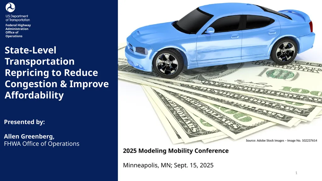
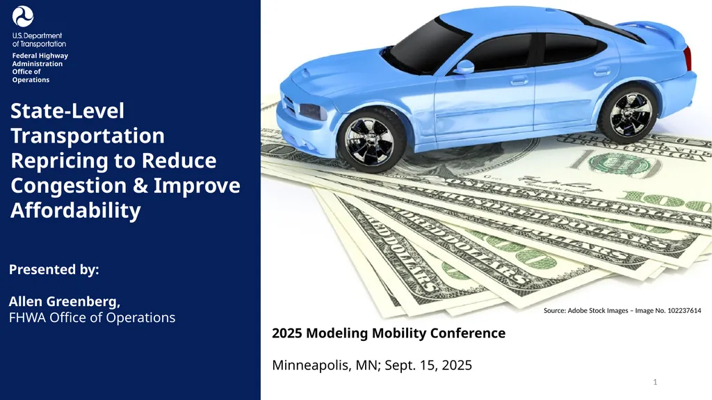
1 State-Level Transportation Repricing to Reduce Congestion & Improve Affordability Presented by:
Allen Greenberg,
FHWA Office of Operations Federal Highway Administration Office of Operations 2025 Modeling Mobility Conference
Minneapolis, MN; Sept. 15, 2025 Source: Adobe Stock Images – Image No. 102237614<br>
Allen Greenberg,
FHWA Office of Operations Federal Highway Administration Office of Operations 2025 Modeling Mobility Conference
Minneapolis, MN; Sept. 15, 2025 Source: Adobe Stock Images – Image No. 102237614<br>
02
Disclaimer The U.S. Government does not endorse products, manufacturers, or outside entities. Trademarks, names, or logos appear here only because they are considered essential to the objective of the presentation. They are included for informational purposes only and are not intended to reflect a preference, approval, or endorsement of any one product or entity.
Except for any statutes or regulations cited, the contents of this presentation do not have the force and effect of law and are not meant to bind the public in any way. This presentation is intended only to provide information regarding existing requirements under the law or agency policies. 2<br>
03
Project Background Reducing vehicle-miles traveled (VMT) offers benefits related to congestion, safety, emissions, and affordability
Flat fees, bundled costs, and parking-only commute benefits encourage driving by keeping the marginal cost of additional vehicle use low
By introducing opportunities to save, transportation repricing strategies (converting fixed transportation costs to variable ones) are effective at reducing VMT through encouraging mode shift and driving discretion
Transportation leaders seek tools to better understand the effects that different state-level choices would have on VMT and related driving externalities 3<br>
04
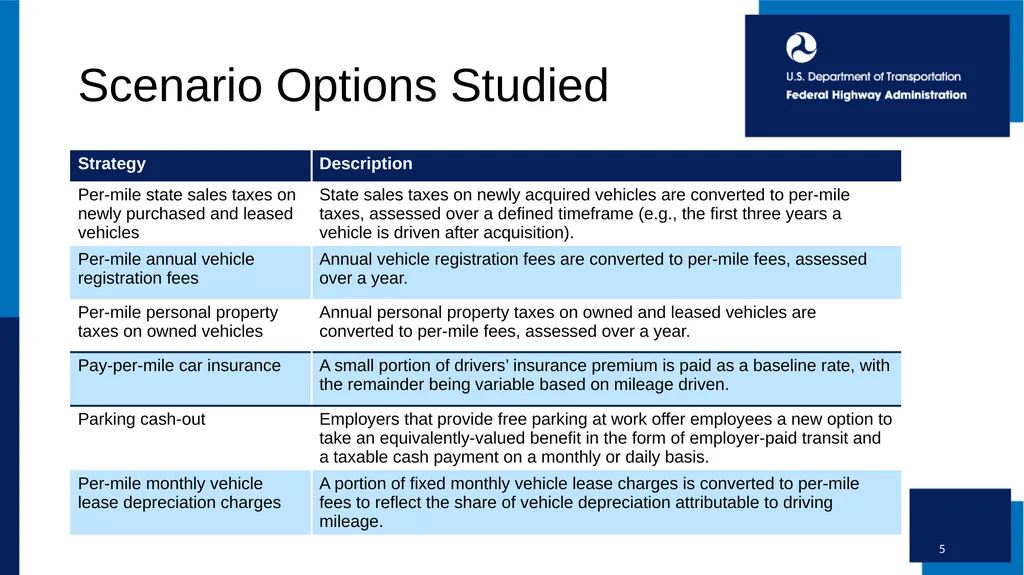
Project Goal Develop a model and supporting report to aid state policymakers in understanding and advancing six repricing strategies
The analysis is in the form of a spreadsheet elasticity model that yields VMT reduction projections for each component of the transportation repricing scenario bundle, and for the bundle as a whole, in each of 50 states and the District of Columbia
VMT reductions are translated to personal cost savings and reductions in congestion, crashes, and other externalities
Effects of the scenarios on transportation affordability are also explored
The model was compared to VisionEval analysis of the policies 4<br>
05
Scenario Options Studied 5<br>
06
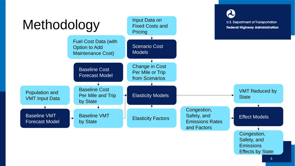
6 VMT Reduced by State Elasticity Models Elasticity Factors Change in Cost Per Mile or Trip from Scenarios Scenario Cost
Models Baseline Cost Forecast Model Fuel Cost Data (with Option to Add Maintenance Cost) Input Data on Fixed Costs and Pricing Baseline VMT
by State Baseline Cost Per Mile and Trip by State Effect Models Congestion, Safety, and Emissions Rates and Factors Congestion, Safety, and Emissions Effects by State Baseline VMT Forecast Model Population and VMT Input Data Methodology<br>
07
Key 7 State Data Input National Data Input Key Assumptions Swap for State- Specific Inputs Model Output Intermediate Value<br>
08
Baseline Cost Per-Mile Model (2030 forecast) Model reflects forecasted 2030 fuel economy.
This model defaults to excluding maintenance expenses in per-mile driving costs, but users can override that choice which would significantly dampen modeled results.
The exclusion is justified because elasticity values derived from observed changes in VMT, responding to changes in driving costs, were typically calculated using only fuel costs.
The 2030 projected baseline fleetwide average per-mile vehicle operating costs incorporate the anticipated degree of vehicle electrification.
Lower electric vehicle operating costs lead to more forecasted baseline driving (as traditionally modeled). 8<br>
09
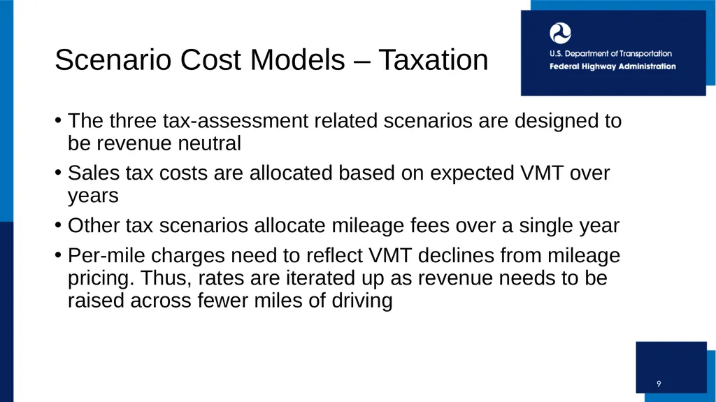
Scenario Cost Models – Taxation The three tax-assessment related scenarios are designed to be revenue neutral
Sales tax costs are allocated based on expected VMT over years
Other tax scenarios allocate mileage fees over a single year
Per-mile charges need to reflect VMT declines from mileage pricing. Thus, rates are iterated up as revenue needs to be raised across fewer miles of driving 9<br>
Sales tax costs are allocated based on expected VMT over years
Other tax scenarios allocate mileage fees over a single year
Per-mile charges need to reflect VMT declines from mileage pricing. Thus, rates are iterated up as revenue needs to be raised across fewer miles of driving 9<br>
10
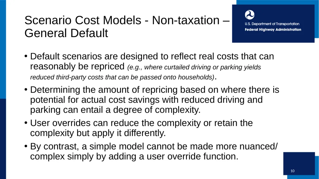
Scenario Cost Models - Non-taxation – General Default Default scenarios are designed to reflect real costs that can reasonably be repriced (e.g., where curtailed driving or parking yields reduced third-party costs that can be passed onto households).
Determining the amount of repricing based on where there is potential for actual cost savings with reduced driving and parking can entail a degree of complexity.
User overrides can reduce the complexity or retain the complexity but apply it differently.
By contrast, a simple model cannot be made more nuanced/ complex simply by adding a user override function. 10<br>
11
Scenario Cost Models - Non-taxation – Default Insurance For pay-per-mile (PPM) insurance, the complexity of the cost model focuses on the proportion of different categories of insurance to reprice.
Liability and collision risk is directly related to mileage, and the default is to reprice 90% of coverage costs to mileage-based (a small portion of coverage costs are strictly related to the number of policies written).
Comprehensive risk is mostly not mileage related (e.g., damage from a storm when a vehicle is parked) but occasionally is (e.g., windshield cracks typically occur when driving). Here, using claims’ causal data, the model defaults to 33% of premiums being mileage-based. 11<br>
12
Scenario Cost Models - Non-taxation –Default Parking Cash-Out Preexisting state-level (e.g., California) and city-level (Washington, DC) parking cash-out requirements inform the default policy that is modeled.
Distinct parking values are used for urban and non-urban areas in each state, using national parking cost data where available or otherwise modeling such costs based on relative housing prices.
The default policy exempts employers with fewer than 10 employees, requires monthly parking cash-out in firms with 10-99 employees, and obligates a daily cash-out offer for employers with 100 or more employees. 12<br>
13
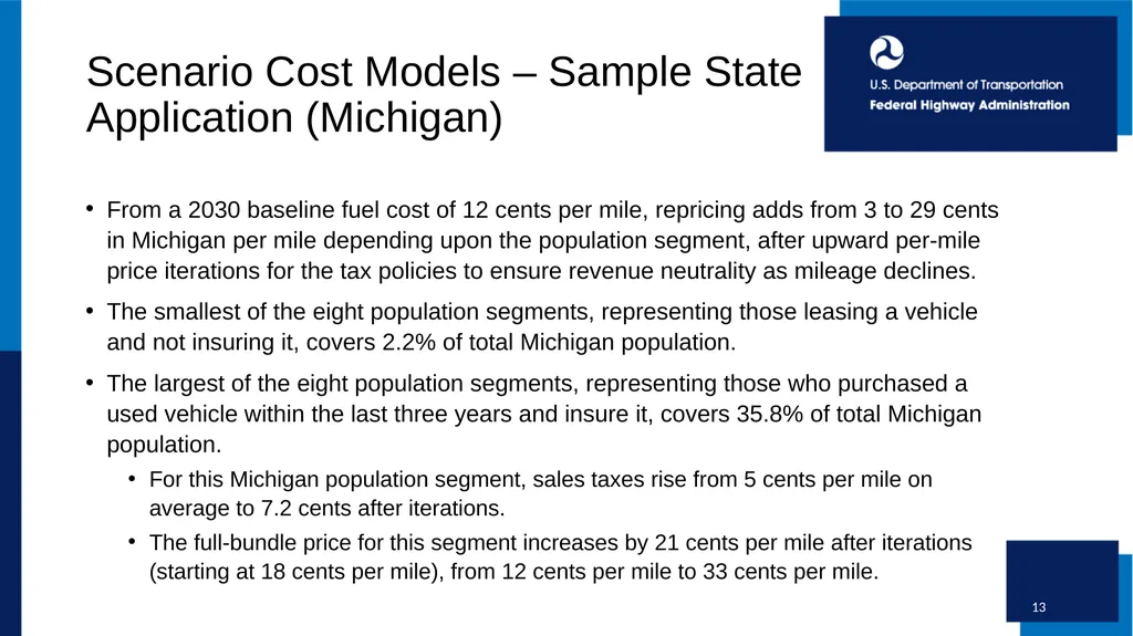
Scenario Cost Models – Sample State Application (Michigan) From a 2030 baseline fuel cost of 12 cents per mile, repricing adds from 3 to 29 cents in Michigan per mile depending upon the population segment, after upward per-mile price iterations for the tax policies to ensure revenue neutrality as mileage declines.
The smallest of the eight population segments, representing those leasing a vehicle and not insuring it, covers 2.2% of total Michigan population.
The largest of the eight population segments, representing those who purchased a used vehicle within the last three years and insure it, covers 35.8% of total Michigan population.
For this Michigan population segment, sales taxes rise from 5 cents per mile on average to 7.2 cents after iterations.
The full-bundle price for this segment increases by 21 cents per mile after iterations (starting at 18 cents per mile), from 12 cents per mile to 33 cents per mile. 13<br>
14
Elasticity Models – Application Ascertaining costs of bundled scenarios and then applying the elasticity function entails:
Total prices per-mile for bundles including all of the five (or fewer in some states) per-mile repricing strategies that apply are calculated for eight distinct market segments.
A -0.3 arc elasticity is applied to the total change in per-mile prices experienced by each market segment. Multiplicative dampening is used when combining impacts of the per-mile repricing strategies with an additional strategy, parking cash-out (for which a -0.3 arc elasticity is also used).
Segments' changes are combined based on their share of total VMT. 14<br>
15
Elasticity Models – Value Selection for Bundles Since the bundle of repricing scenarios that are modeled has never been implemented, it creates a challenge in selecting an appropriate elasticity value.
This is not an issue for selecting elasticity values for individual scenarios, where cost changes previously experienced in the marketplace have been of a similar magnitude.
An appropriate question: Is it right to use the same elasticity value when projecting impacts of a single repricing scenario versus a bundle of repricing scenarios?
The closest (albeit imperfect) big changes in driving prices experienced in the marketplace are of three types: (1) experiments where users were given “bank accounts” for which sometimes-high mileage and toll prices (specific to the user) were deducted, and the user was allowed to cash-out unspent money in their accounts after completion of the experiments; (2) newly introduced cordon pricing, such as in London, Stockholm, and Singapore, very significantly increasing the costs drivers would incur in specific travel zones at applicable times; and (3) surge pricing for ridehail trips.
Data from such studies support the selection of an elasticity value equivalent to, or even higher than, the default elasticity of -0.3 selected for modeling of individual scenarios. 15<br>
16
Effect Models Applying an elasticity function to model impacts of repricing would yield a bigger reduction in driving mileage of electric versus other vehicles (due to repricing representing a higher percentage increase in driving costs). This is reflected in the projected overall results.
For the purpose of projecting externality impacts, distinguishing factors are retained and used.
Examples include urban versus non-urban driving, parking value variability, commute and non-commute trips, and driving of new vehicles (which are more likely to be electric and/or less polluting, but are also driven more) versus older vehicles.
This matters most especially for repricing scenarios that disproportionately impact newer vehicles (i.e., repricing sales taxes, where per-mile costs reflect vehicle purchase prices). Here, reduced VMT yields proportionately reduced environmental benefit due to newer vehicles being less emitting/polluting. 16<br>
17
Complex Interactions (Cheaper Used Vehicle Acquisition) Repricing eliminates some upfront costs, making vehicle acquisition and insurance more affordable. This has complex impacts on costs for low-income households and on overall VMT.
Some will gain new access to a vehicle, which could be very important for securing jobs and other opportunities, but also grows VMT (although limited due to low-income populations tending to drive less than average combined with high per-mile pricing to which they would be particularly sensitive).
Those getting vehicle access due only to reduced upfront costs are assumed as starting out in the 25th percentile of VMT.
Like with all populations, VMT is then reduced reflective of scenario costs and the application of the price elasticity function (resulting overall new VMT from this population is subtracted from the reductions from all other populations). 17<br>
18
Complex Interactions (Cheaper Auto Insurance) Pay-per-mile insurance is assumed to decrease the percentage of motorists who choose to remain uninsured by 36%, reflective of data from New Jersey which added a significantly cheaper public option insurance product.
Low-income households driving with no insurance because they cannot afford the high upfront costs are incurring great legal risk, possibly including incarceration, and some would take advantage of PPM offerings to buy insurance only for the miles that they drive to eliminate this legal risk.
Costs associated with low-income households choosing to purchase insurance or vehicles due to repricing eliminating upfront costs do not detract from affordability. Absent repricing, such household would be without a vehicle or driving uninsured. 18<br>
19
Study Model Results 19<br>
20
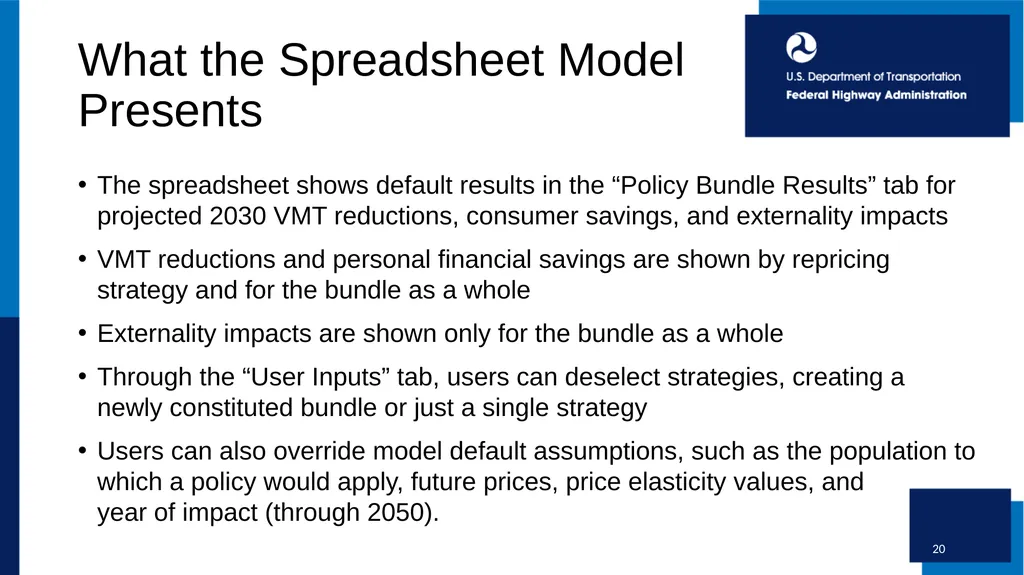
What the Spreadsheet Model Presents The spreadsheet shows default results in the “Policy Bundle Results” tab for projected 2030 VMT reductions, consumer savings, and externality impacts
VMT reductions and personal financial savings are shown by repricing strategy and for the bundle as a whole
Externality impacts are shown only for the bundle as a whole
Through the “User Inputs” tab, users can deselect strategies, creating a newly constituted bundle or just a single strategy
Users can also override model default assumptions, such as the population to which a policy would apply, future prices, price elasticity values, and year of impact (through 2050). 20<br>
21
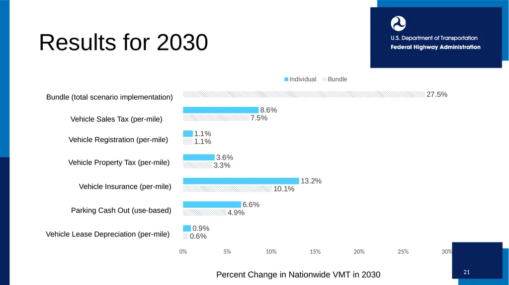
Results for 2030 21 Vehicle Sales Tax (per-mile) Bundle (total scenario implementation) Vehicle Lease Depreciation (per-mile) Parking Cash Out (use-based) Vehicle Insurance (per-mile) Vehicle Property Tax (per-mile) Vehicle Registration (per-mile) Percent Change in Nationwide VMT in 2030<br>
22
Results for 2030:
Individual Scenarios 22<br>
23
Results for 2030:
Percent Change in VMT 23<br>
24
Results for 2030:
Tax Repricing Mini-Bundle 24 Overall Impact Sales Tax Repricing Personal Property Tax Repricing Registration Fee Repricing Percent Change in Nationwide VMT in 2030<br>
25
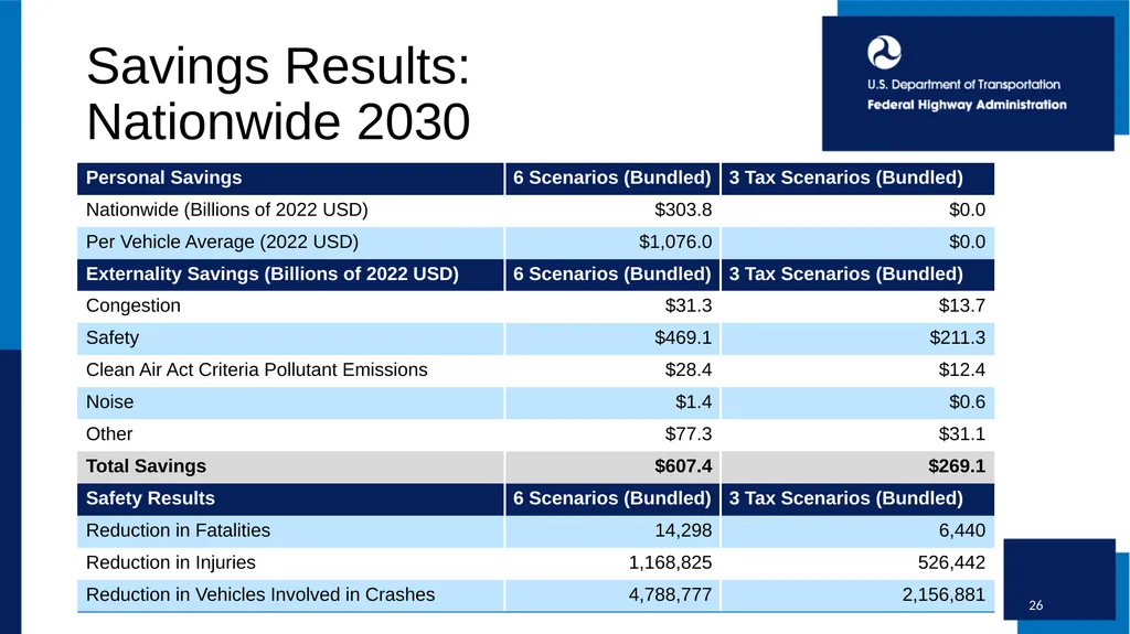
Externality Benefits Safety based on USDOT Guidance on Evaluation of Statistical Life in Economic Analysis. Crash reductions based on average national rates from Bureau of Transportation Statistics for occupant injuries adjusted to include non-occupancy impacts.
Criterial Pollutant, Congestion and Noise Benefits based on FHWA’s External Costs of Transportation (ECAT) database for state-specific atmospheric, density, and roadway network characteristics.
Modeled 2030 benefits for Safety and Emissions are based on the national vehicle fleet; projections on how fleet characteristics may vary from state to state were not made. 25<br>
26
Savings Results:
Nationwide 2030 26<br>
27
Questions & Contact Questions may be directed to:
Allen Greenberg FHWA Office of Operations Allen.Greenberg@dot.gov 27<br>
Allen Greenberg FHWA Office of Operations Allen.Greenberg@dot.gov 27<br>