
1 Theory: Models of Computation Readings: Chapter
T
Published · 50 slides · 0 views

1 / 1

Description
1 Theory: Models of Computation Readings: Chapter 11 Chapter 3.6 of SG Content: What is a Model Model of Computation Model of a Computing Agent Model of an Algorithm TM Program Examples Computability (Church-Turing Thesis) Computational
Related Topics
Share
Embed code
Download this presentation From Below
"1 Theory: Models of Computation Readings: Chapter" is the property of its rightful owner. Permission is granted to download and print the materials on this website for personal, non-commercial use only, and to display it on your personal computer provided you do not modify the materials and that you retain all copyright notices contained in the materials. By downloading content from our website, you accept the terms of this agreement.
Presentation Transcript
01
1 Theory: Models of Computation Readings:
Chapter 11 & Chapter 3.6 of [SG]
Content:
What is a Model
Model of Computation
Model of a Computing Agent
Model of an Algorithm
TM Program Examples
Computability (Church-Turing Thesis)
Computational Complexity of Problems<br>
Chapter 11 & Chapter 3.6 of [SG]
Content:
What is a Model
Model of Computation
Model of a Computing Agent
Model of an Algorithm
TM Program Examples
Computability (Church-Turing Thesis)
Computational Complexity of Problems<br>
02
2 Theory: Goals To give a model of computation
to be able to reason about the capabilities of computers
To study the properties of computation
rather than being lost in the details of the machine hw/sw
To study
what computers may be able to do, and
what they cannot do
To study
What can be done quickly, and
what cannot be done quickly<br>
to be able to reason about the capabilities of computers
To study the properties of computation
rather than being lost in the details of the machine hw/sw
To study
what computers may be able to do, and
what they cannot do
To study
What can be done quickly, and
what cannot be done quickly<br>
03
3 Self Readings: Section 11.1 – 11.3.1
Introduction, Models, Computing Agents<br>
Introduction, Models, Computing Agents<br>
04
4 Theory: Models of Computation Content:
What is a Model
Model of Computation
Model of a Computing Agent
Model of an Algorithm
TM Program Examples
Computability (Church-Turing Thesis)
Computational Complexity of Problems<br>
What is a Model
Model of Computation
Model of a Computing Agent
Model of an Algorithm
TM Program Examples
Computability (Church-Turing Thesis)
Computational Complexity of Problems<br>
05
5 Theory: Goals We will construct a model of computation.
A simple, functional description of a computer
to capture essence of computation
suppress details
easy to study and reason about
Turing Machine
(there are several other models)<br>
A simple, functional description of a computer
to capture essence of computation
suppress details
easy to study and reason about
Turing Machine
(there are several other models)<br>
06
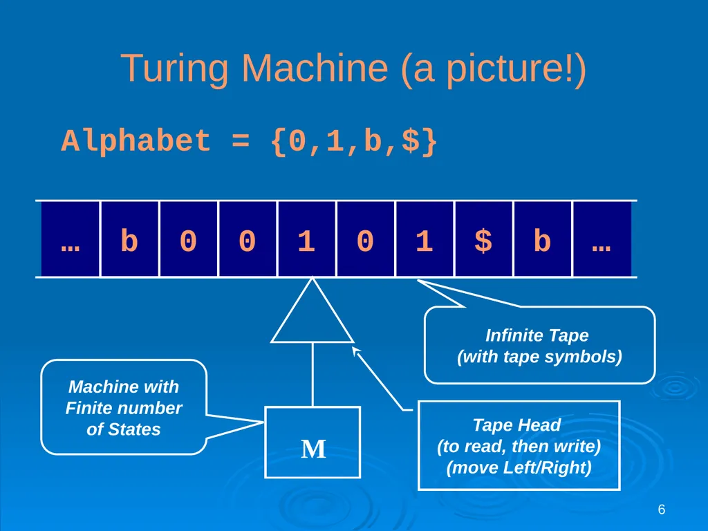
6 Turing Machine (a picture!) Infinite Tape
(with tape symbols) Alphabet = {0,1,b,$} Machine with Finite number of States Tape Head (to read, then write)
(move Left/Right)<br>
(with tape symbols) Alphabet = {0,1,b,$} Machine with Finite number of States Tape Head (to read, then write)
(move Left/Right)<br>
07
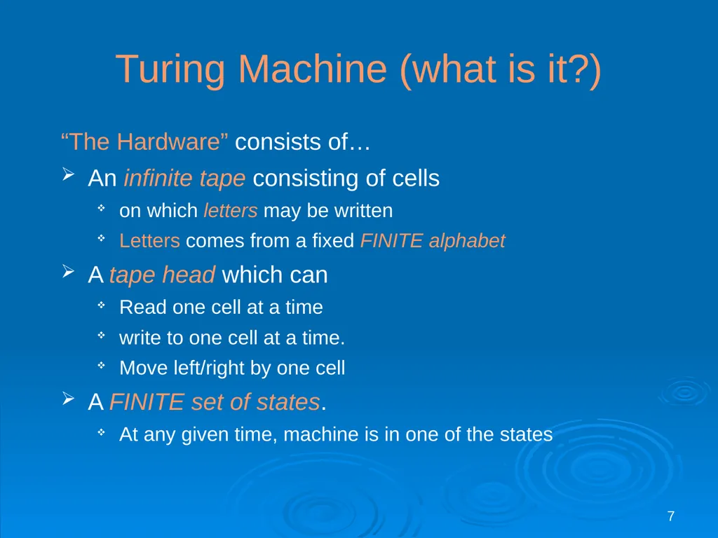
7 Turing Machine (what is it?) “The Hardware” consists of…
An infinite tape consisting of cells
on which letters may be written
Letters comes from a fixed FINITE alphabet
A tape head which can
Read one cell at a time
write to one cell at a time.
Move left/right by one cell
A FINITE set of states.
At any given time, machine is in one of the states<br>
An infinite tape consisting of cells
on which letters may be written
Letters comes from a fixed FINITE alphabet
A tape head which can
Read one cell at a time
write to one cell at a time.
Move left/right by one cell
A FINITE set of states.
At any given time, machine is in one of the states<br>
08
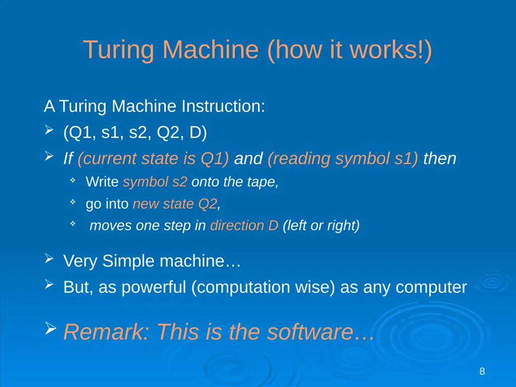
8 Turing Machine (how it works!) A Turing Machine Instruction:
(Q1, s1, s2, Q2, D)
If (current state is Q1) and (reading symbol s1) then
Write symbol s2 onto the tape,
go into new state Q2,
moves one step in direction D (left or right)
Very Simple machine…
But, as powerful (computation wise) as any computer
Remark: This is the software…<br>
(Q1, s1, s2, Q2, D)
If (current state is Q1) and (reading symbol s1) then
Write symbol s2 onto the tape,
go into new state Q2,
moves one step in direction D (left or right)
Very Simple machine…
But, as powerful (computation wise) as any computer
Remark: This is the software…<br>
09
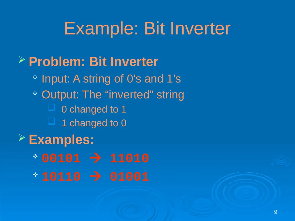
9 Example: Bit Inverter Problem: Bit Inverter
Input: A string of 0’s and 1’s
Output: The “inverted” string
0 changed to 1
1 changed to 0
Examples:
00101 11010
10110 01001<br>
Input: A string of 0’s and 1’s
Output: The “inverted” string
0 changed to 1
1 changed to 0
Examples:
00101 11010
10110 01001<br>
10
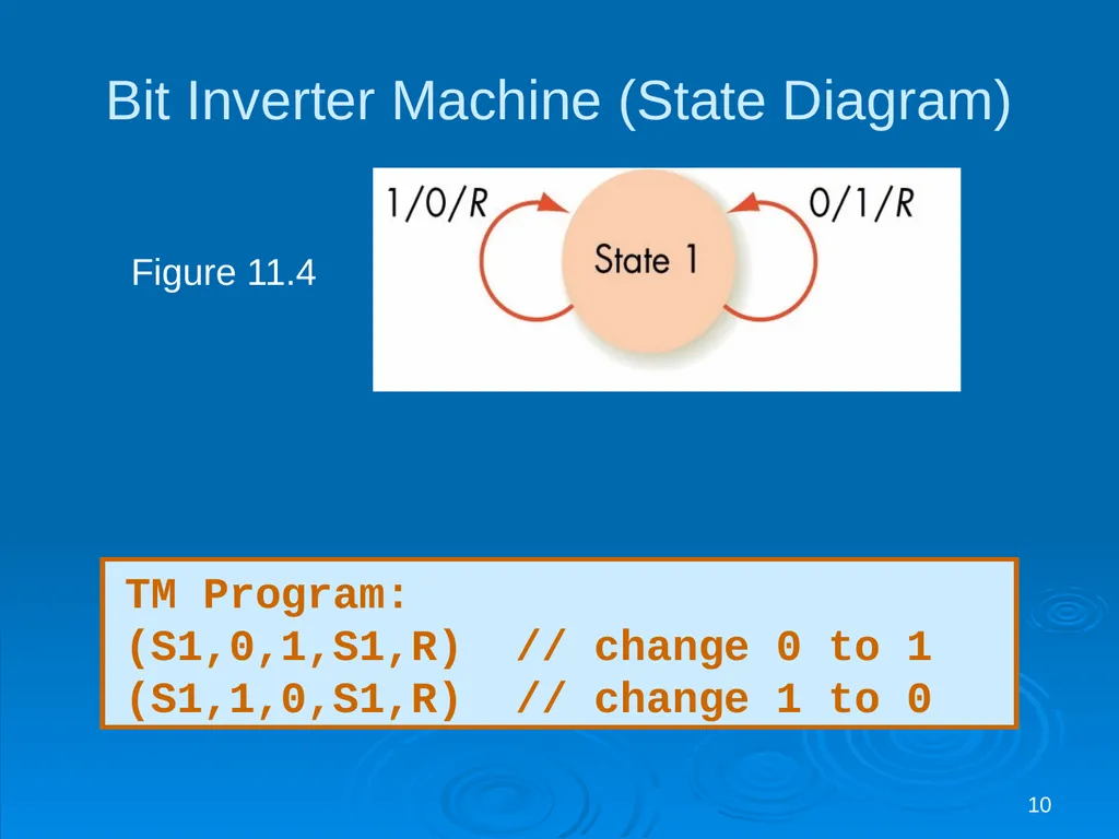
10 Figure 11.4 TM Program:
(S1,0,1,S1,R) // change 0 to 1
(S1,1,0,S1,R) // change 1 to 0 Bit Inverter Machine (State Diagram)<br>
(S1,0,1,S1,R) // change 0 to 1
(S1,1,0,S1,R) // change 1 to 0 Bit Inverter Machine (State Diagram)<br>
11
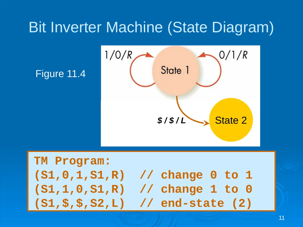
11 Figure 11.4 TM Program:
(S1,0,1,S1,R) // change 0 to 1
(S1,1,0,S1,R) // change 1 to 0
(S1,$,$,S2,L) // end-state (2) Bit Inverter Machine (State Diagram)<br>
(S1,0,1,S1,R) // change 0 to 1
(S1,1,0,S1,R) // change 1 to 0
(S1,$,$,S2,L) // end-state (2) Bit Inverter Machine (State Diagram)<br>
12
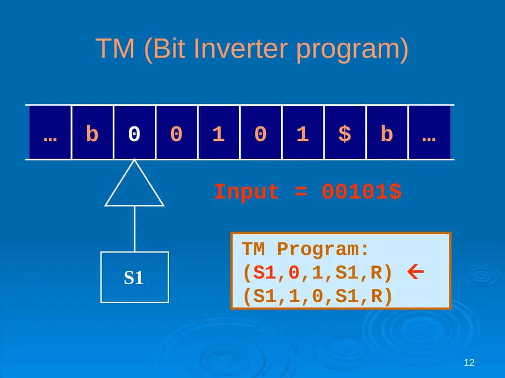
12 TM (Bit Inverter program) TM Program:
(S1,0,1,S1,R)
(S1,1,0,S1,R) Input = 00101$<br>
(S1,0,1,S1,R)
(S1,1,0,S1,R) Input = 00101$<br>
13
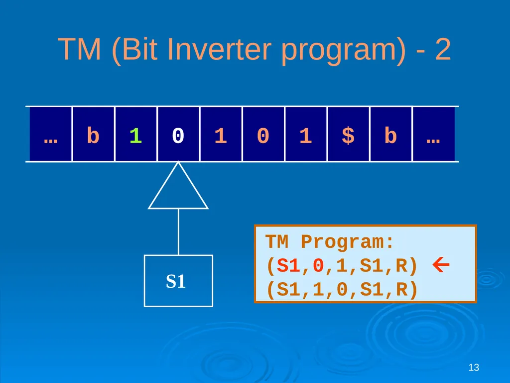
13 TM (Bit Inverter program) - 2 TM Program:
(S1,0,1,S1,R)
(S1,1,0,S1,R)<br>
(S1,0,1,S1,R)
(S1,1,0,S1,R)<br>
14
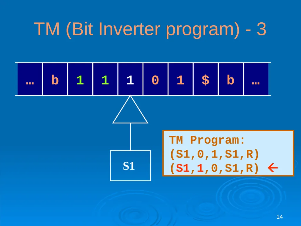
14 TM (Bit Inverter program) - 3 TM Program:
(S1,0,1,S1,R)
(S1,1,0,S1,R) <br>
(S1,0,1,S1,R)
(S1,1,0,S1,R) <br>
15
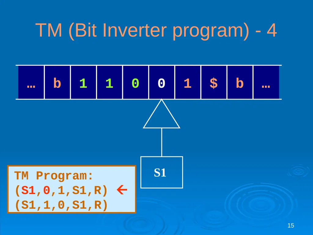
15 TM (Bit Inverter program) - 4 TM Program:
(S1,0,1,S1,R)
(S1,1,0,S1,R)<br>
(S1,0,1,S1,R)
(S1,1,0,S1,R)<br>
16
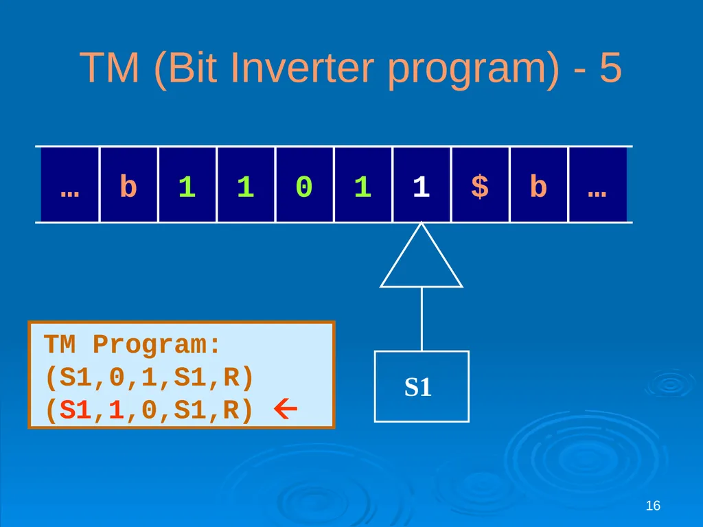
16 TM (Bit Inverter program) - 5 TM Program:
(S1,0,1,S1,R)
(S1,1,0,S1,R) <br>
(S1,0,1,S1,R)
(S1,1,0,S1,R) <br>
17
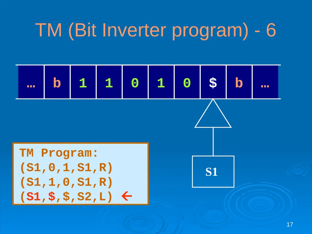
17 TM (Bit Inverter program) - 6 TM Program:
(S1,0,1,S1,R)
(S1,1,0,S1,R)
(S1,$,$,S2,L) <br>
(S1,0,1,S1,R)
(S1,1,0,S1,R)
(S1,$,$,S2,L) <br>
18
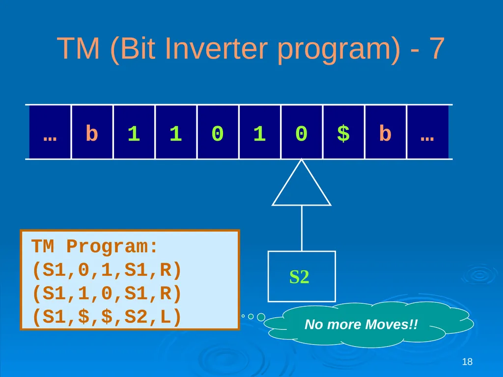
18 TM (Bit Inverter program) - 7 TM Program:
(S1,0,1,S1,R)
(S1,1,0,S1,R)
(S1,$,$,S2,L) No more Moves!!<br>
(S1,0,1,S1,R)
(S1,1,0,S1,R)
(S1,$,$,S2,L) No more Moves!!<br>
19
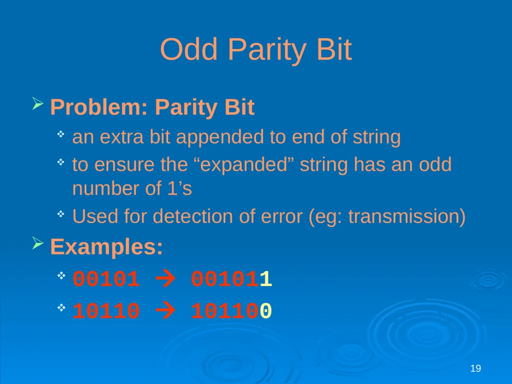
19 Odd Parity Bit Problem: Parity Bit
an extra bit appended to end of string
to ensure the “expanded” string has an odd number of 1’s
Used for detection of error (eg: transmission)
Examples:
00101 001011
10110 101100<br>
an extra bit appended to end of string
to ensure the “expanded” string has an odd number of 1’s
Used for detection of error (eg: transmission)
Examples:
00101 001011
10110 101100<br>
20
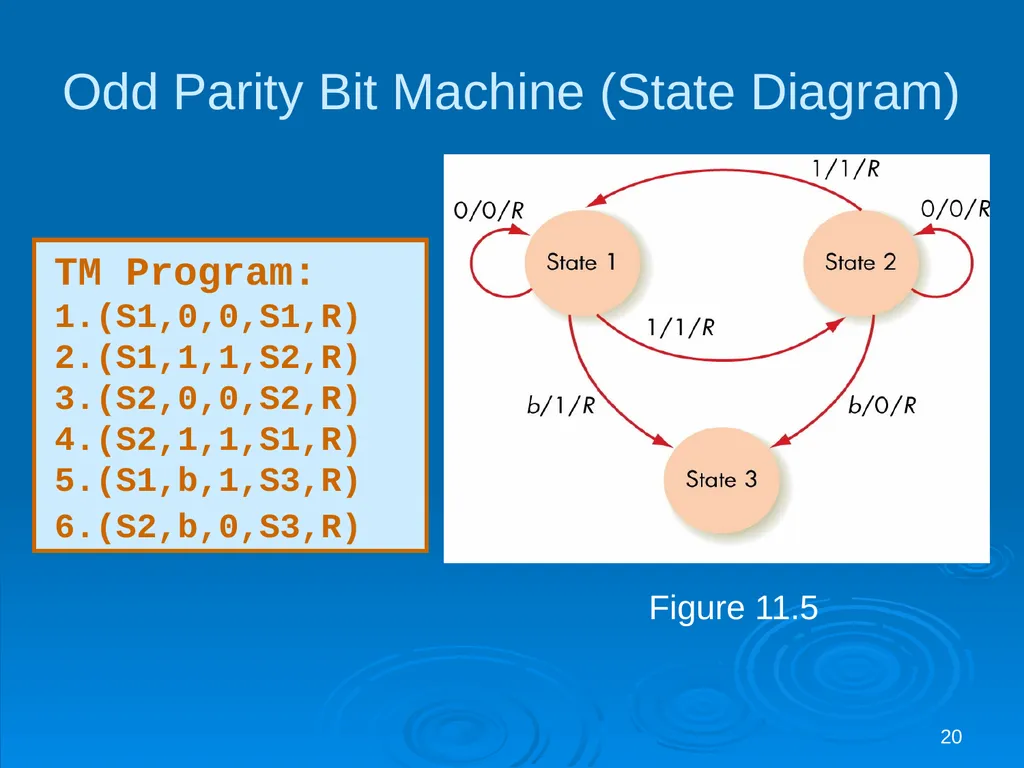
20 Figure 11.5 TM Program:
1.(S1,0,0,S1,R)
2.(S1,1,1,S2,R)
3.(S2,0,0,S2,R)
4.(S2,1,1,S1,R)
5.(S1,b,1,S3,R)
6.(S2,b,0,S3,R) Odd Parity Bit Machine (State Diagram)<br>
1.(S1,0,0,S1,R)
2.(S1,1,1,S2,R)
3.(S2,0,0,S2,R)
4.(S2,1,1,S1,R)
5.(S1,b,1,S3,R)
6.(S2,b,0,S3,R) Odd Parity Bit Machine (State Diagram)<br>
21
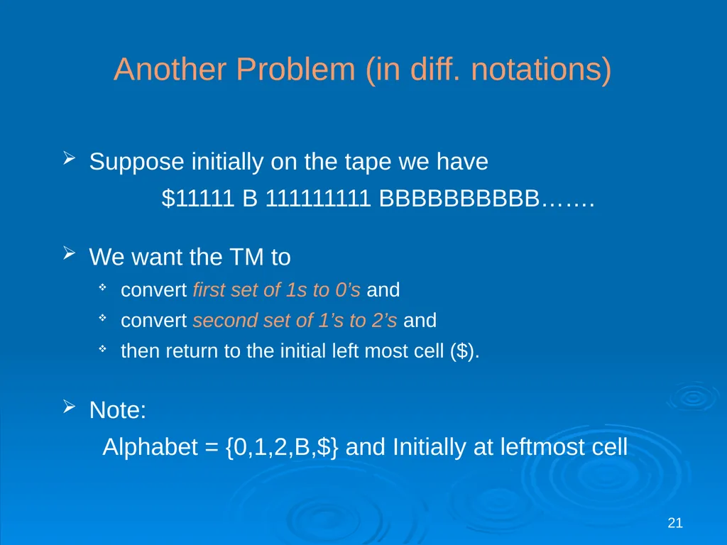
21 Another Problem (in diff. notations) Suppose initially on the tape we have
$11111 B 111111111 BBBBBBBBBB…….
We want the TM to
convert first set of 1s to 0’s and
convert second set of 1’s to 2’s and
then return to the initial left most cell ($).
Note:
Alphabet = {0,1,2,B,$} and Initially at leftmost cell<br>
$11111 B 111111111 BBBBBBBBBB…….
We want the TM to
convert first set of 1s to 0’s and
convert second set of 1’s to 2’s and
then return to the initial left most cell ($).
Note:
Alphabet = {0,1,2,B,$} and Initially at leftmost cell<br>
22
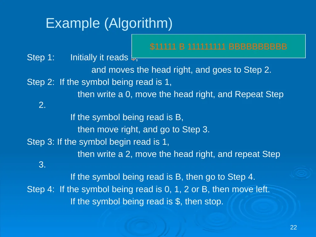
22 Example (Algorithm) Step 1: Initially it reads $,
and moves the head right, and goes to Step 2.
Step 2: If the symbol being read is 1,
then write a 0, move the head right, and Repeat Step 2.
If the symbol being read is B,
then move right, and go to Step 3.
Step 3: If the symbol begin read is 1,
then write a 2, move the head right, and repeat Step 3.
If the symbol being read is B, then go to Step 4.
Step 4: If the symbol being read is 0, 1, 2 or B, then move left.
If the symbol being read is $, then stop. $11111 B 111111111 BBBBBBBBBB<br>
and moves the head right, and goes to Step 2.
Step 2: If the symbol being read is 1,
then write a 0, move the head right, and Repeat Step 2.
If the symbol being read is B,
then move right, and go to Step 3.
Step 3: If the symbol begin read is 1,
then write a 2, move the head right, and repeat Step 3.
If the symbol being read is B, then go to Step 4.
Step 4: If the symbol being read is 0, 1, 2 or B, then move left.
If the symbol being read is $, then stop. $11111 B 111111111 BBBBBBBBBB<br>
23
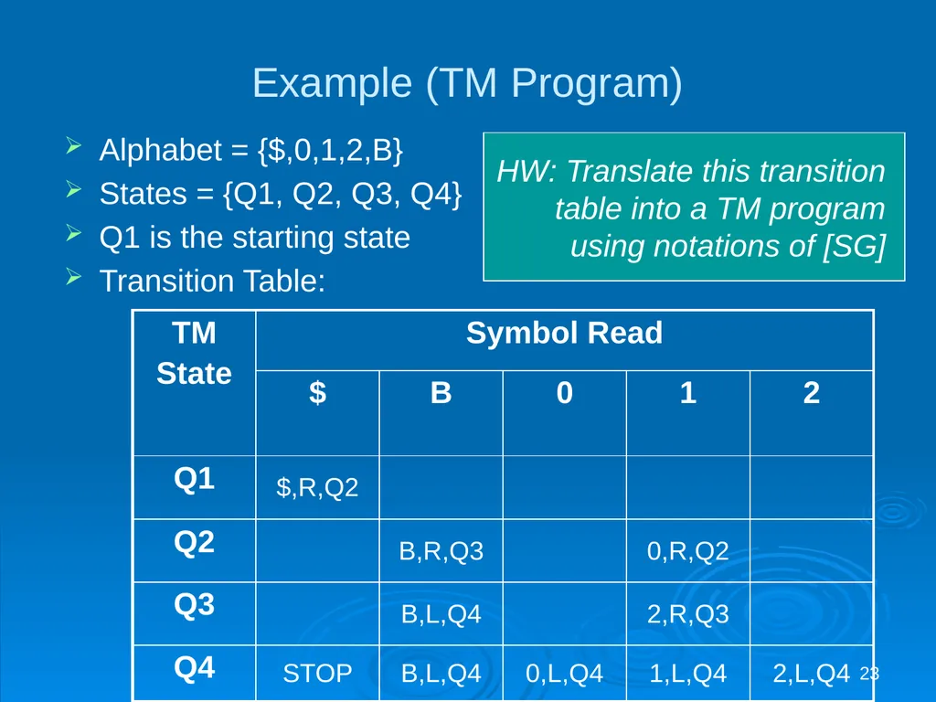
23 Example (TM Program) Alphabet = {$,0,1,2,B}
States = {Q1, Q2, Q3, Q4}
Q1 is the starting state
Transition Table: HW: Translate this transition
table into a TM program
using notations of [SG]<br>
States = {Q1, Q2, Q3, Q4}
Q1 is the starting state
Transition Table: HW: Translate this transition
table into a TM program
using notations of [SG]<br>
24
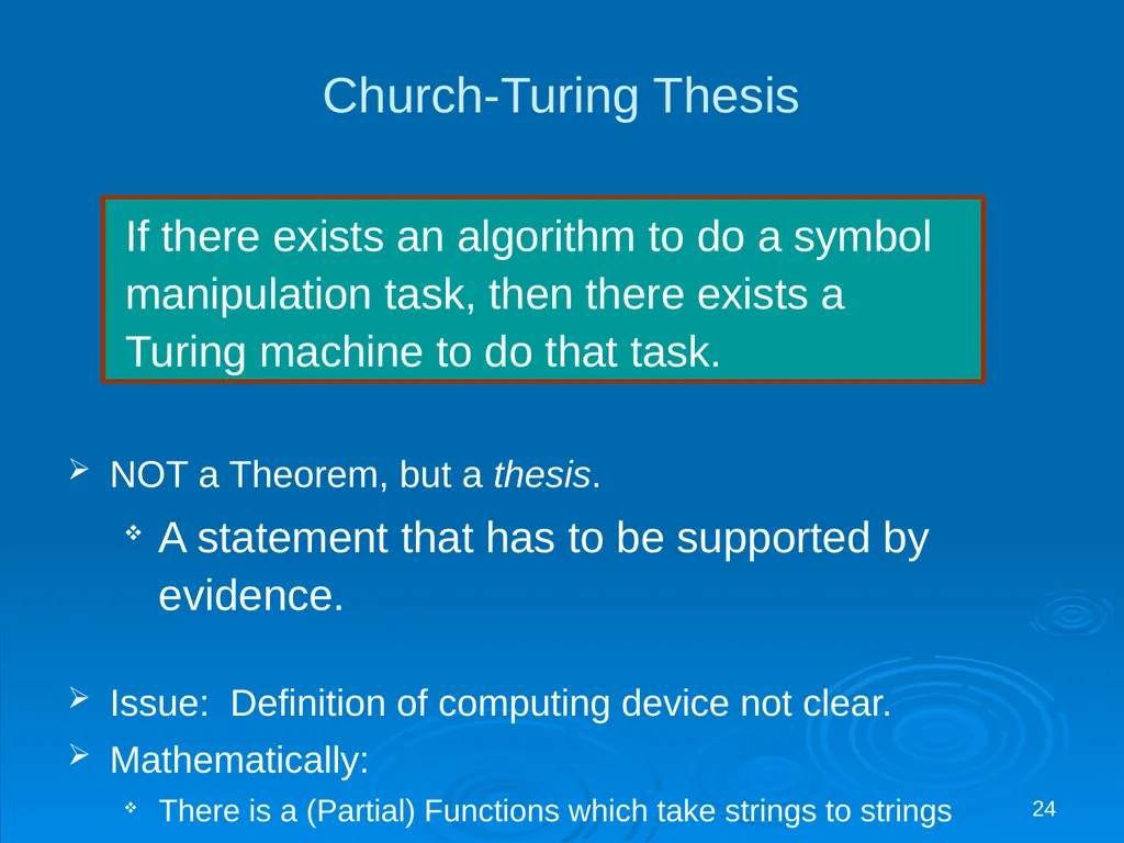
24 Church-Turing Thesis NOT a Theorem, but a thesis.
A statement that has to be supported by evidence.
Issue: Definition of computing device not clear.
Mathematically:
There is a (Partial) Functions which take strings to strings If there exists an algorithm to do a symbol manipulation task, then there exists a Turing machine to do that task.<br>
A statement that has to be supported by evidence.
Issue: Definition of computing device not clear.
Mathematically:
There is a (Partial) Functions which take strings to strings If there exists an algorithm to do a symbol manipulation task, then there exists a Turing machine to do that task.<br>
25
25 Church-Turing Thesis (cont) Two parts to writing a Turing machine for a symbol manipulation task
Encoding symbolic information as strings of 0s and 1s (eg: numbers, sound, pictures, etc)
Writing the Turing machine instructions to produce the encoded form of the output<br>
Encoding symbolic information as strings of 0s and 1s (eg: numbers, sound, pictures, etc)
Writing the Turing machine instructions to produce the encoded form of the output<br>
26
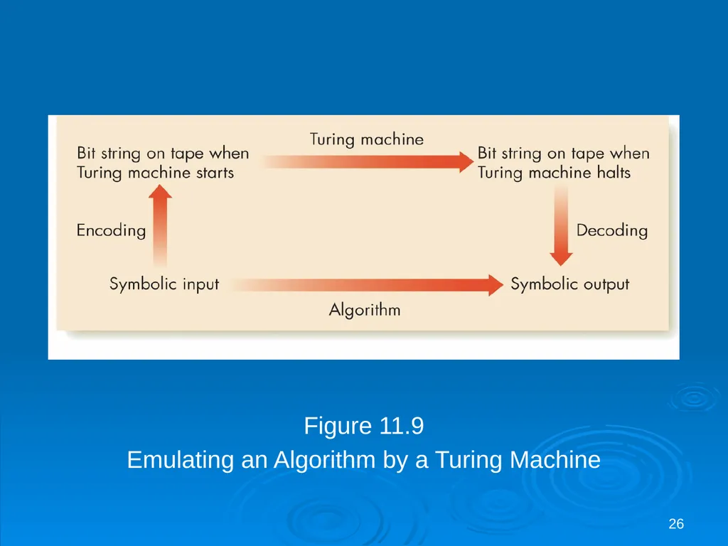
26 Figure 11.9
Emulating an Algorithm by a Turing Machine<br>
Emulating an Algorithm by a Turing Machine<br>
27
27 Limits of Computabiltiy: Based on Church-Turing thesis,
TM defines limits of computability
TM = ultimate model of computing agent
TM program = ultimate model of algorithm
Are all problems solvable using a TM?
Uncomputable or unsolvable problems
problem for which we can prove that no TM exists that will solve it.<br>
TM = ultimate model of computing agent
TM program = ultimate model of algorithm
Are all problems solvable using a TM?
Uncomputable or unsolvable problems
problem for which we can prove that no TM exists that will solve it.<br>
28
28 Computability Q: Can we solve every problem?
In Mathematics:
Godel’s Theorem: Not every true theorem about natural numbers can be proven.
In Computer Science:
Not every problem can be solved.
Example: Halting Problem<br>
In Mathematics:
Godel’s Theorem: Not every true theorem about natural numbers can be proven.
In Computer Science:
Not every problem can be solved.
Example: Halting Problem<br>
29
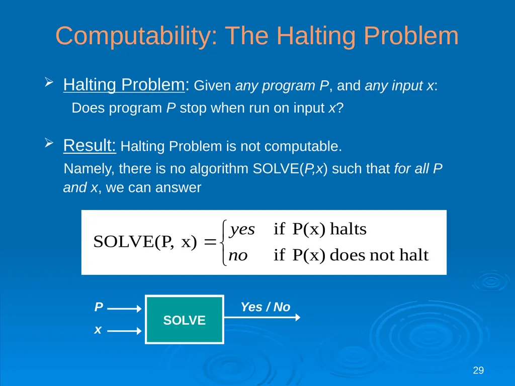
29 Computability: The Halting Problem Halting Problem: Given any program P, and any input x:
Does program P stop when run on input x?
Result: Halting Problem is not computable.
Namely, there is no algorithm SOLVE(P,x) such that for all P and x, we can answer<br>
Does program P stop when run on input x?
Result: Halting Problem is not computable.
Namely, there is no algorithm SOLVE(P,x) such that for all P and x, we can answer<br>
30
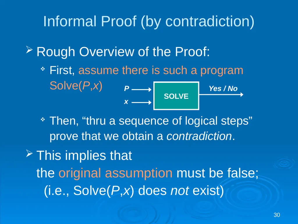
30 Informal Proof (by contradiction) Rough Overview of the Proof:
First, assume there is such a program Solve(P,x)
Then, “thru a sequence of logical steps” prove that we obtain a contradiction.
This implies that the original assumption must be false; (i.e., Solve(P,x) does not exist)<br>
First, assume there is such a program Solve(P,x)
Then, “thru a sequence of logical steps” prove that we obtain a contradiction.
This implies that the original assumption must be false; (i.e., Solve(P,x) does not exist)<br>
31
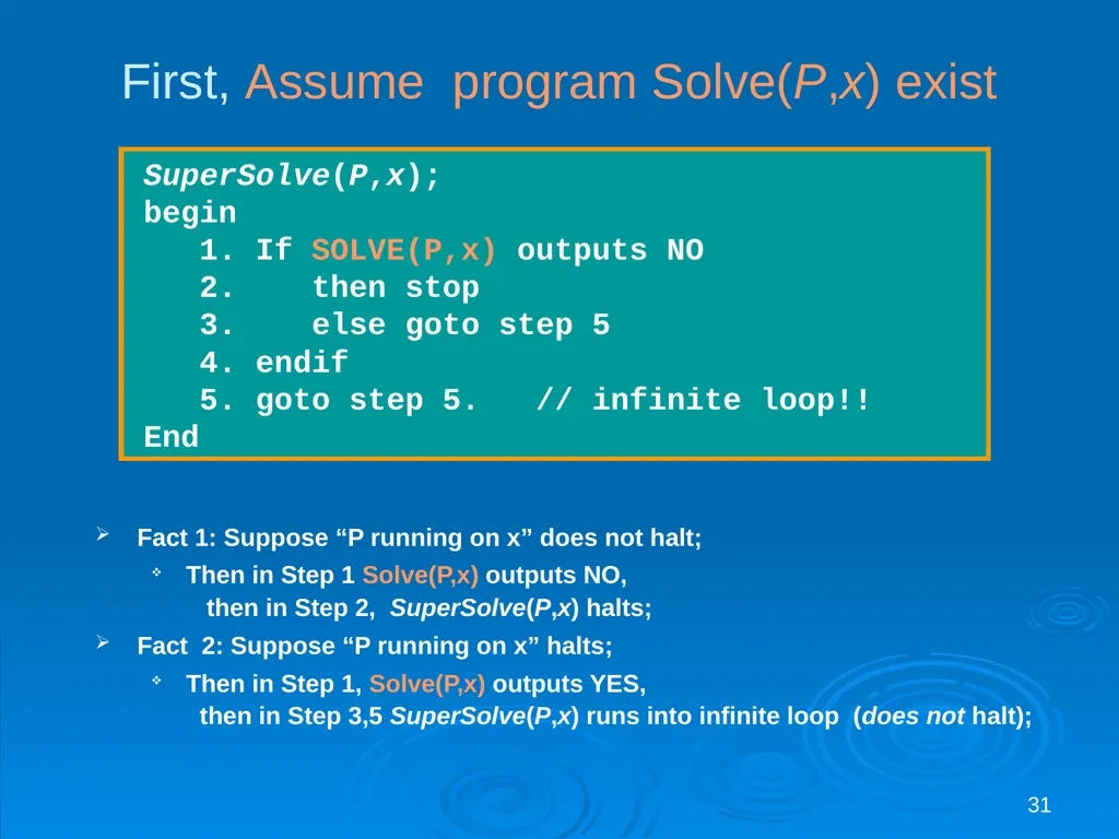
31 First, Assume program Solve(P,x) exist Fact 1: Suppose “P running on x” does not halt;
Then in Step 1 Solve(P,x) outputs NO, then in Step 2, SuperSolve(P,x) halts;
Fact 2: Suppose “P running on x” halts;
Then in Step 1, Solve(P,x) outputs YES, then in Step 3,5 SuperSolve(P,x) runs into infinite loop (does not halt); SuperSolve(P,x);
begin
1. If SOLVE(P,x) outputs NO
2. then stop
3. else goto step 5
4. endif
5. goto step 5. // infinite loop!!
End<br>
Then in Step 1 Solve(P,x) outputs NO, then in Step 2, SuperSolve(P,x) halts;
Fact 2: Suppose “P running on x” halts;
Then in Step 1, Solve(P,x) outputs YES, then in Step 3,5 SuperSolve(P,x) runs into infinite loop (does not halt); SuperSolve(P,x);
begin
1. If SOLVE(P,x) outputs NO
2. then stop
3. else goto step 5
4. endif
5. goto step 5. // infinite loop!!
End<br>
32
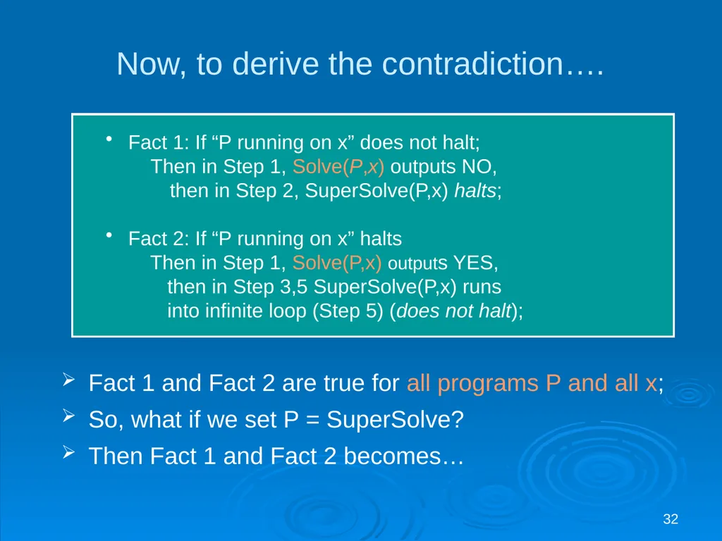
32 Fact 1: If “P running on x” does not halt;
Then in Step 1, Solve(P,x) outputs NO,
then in Step 2, SuperSolve(P,x) halts;
Fact 2: If “P running on x” halts Then in Step 1, Solve(P,x) outputs YES, then in Step 3,5 SuperSolve(P,x) runs into infinite loop (Step 5) (does not halt); Now, to derive the contradiction…. Fact 1 and Fact 2 are true for all programs P and all x;
So, what if we set P = SuperSolve?
Then Fact 1 and Fact 2 becomes…<br>
Then in Step 1, Solve(P,x) outputs NO,
then in Step 2, SuperSolve(P,x) halts;
Fact 2: If “P running on x” halts Then in Step 1, Solve(P,x) outputs YES, then in Step 3,5 SuperSolve(P,x) runs into infinite loop (Step 5) (does not halt); Now, to derive the contradiction…. Fact 1 and Fact 2 are true for all programs P and all x;
So, what if we set P = SuperSolve?
Then Fact 1 and Fact 2 becomes…<br>
33
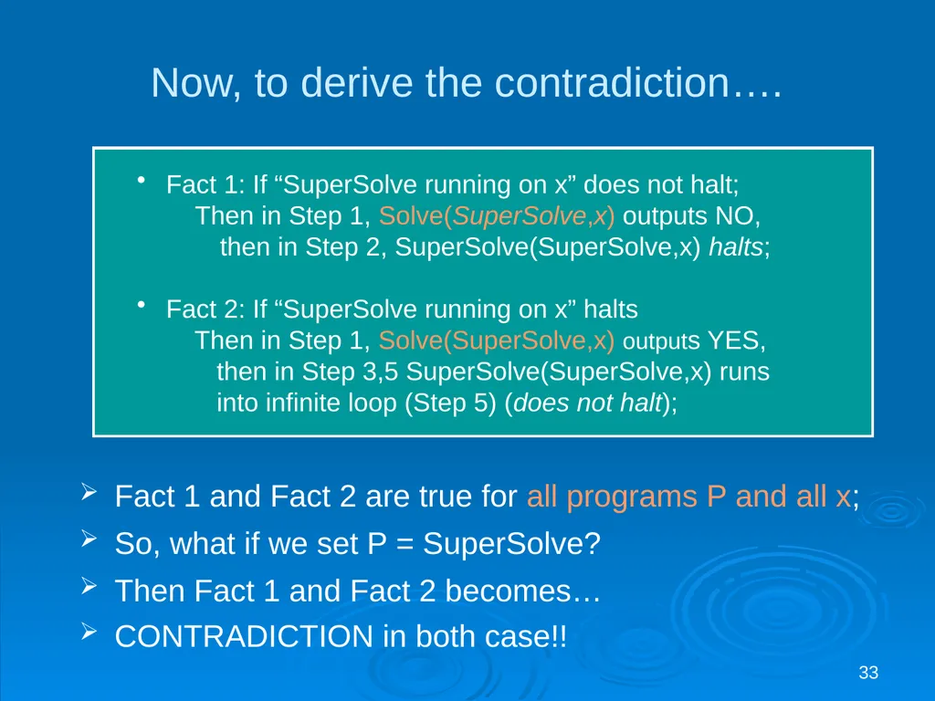
33 Now, to derive the contradiction…. Fact 1 and Fact 2 are true for all programs P and all x;
So, what if we set P = SuperSolve?
Then Fact 1 and Fact 2 becomes… Fact 1: If “SuperSolve running on x” does not halt;
Then in Step 1, Solve(SuperSolve,x) outputs NO,
then in Step 2, SuperSolve(SuperSolve,x) halts;
Fact 2: If “SuperSolve running on x” halts Then in Step 1, Solve(SuperSolve,x) outputs YES, then in Step 3,5 SuperSolve(SuperSolve,x) runs into infinite loop (Step 5) (does not halt); CONTRADICTION in both case!!<br>
So, what if we set P = SuperSolve?
Then Fact 1 and Fact 2 becomes… Fact 1: If “SuperSolve running on x” does not halt;
Then in Step 1, Solve(SuperSolve,x) outputs NO,
then in Step 2, SuperSolve(SuperSolve,x) halts;
Fact 2: If “SuperSolve running on x” halts Then in Step 1, Solve(SuperSolve,x) outputs YES, then in Step 3,5 SuperSolve(SuperSolve,x) runs into infinite loop (Step 5) (does not halt); CONTRADICTION in both case!!<br>
34
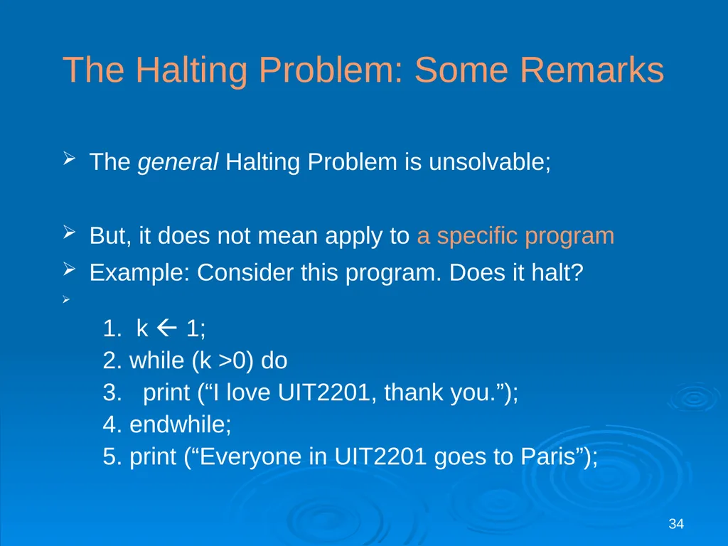
34 The Halting Problem: Some Remarks The general Halting Problem is unsolvable;
But, it does not mean apply to a specific program
Example: Consider this program. Does it halt?
1. k 1; 2. while (k >0) do 3. print (“I love UIT2201, thank you.”); 4. endwhile; 5. print (“Everyone in UIT2201 goes to Paris”);<br>
But, it does not mean apply to a specific program
Example: Consider this program. Does it halt?
1. k 1; 2. while (k >0) do 3. print (“I love UIT2201, thank you.”); 4. endwhile; 5. print (“Everyone in UIT2201 goes to Paris”);<br>
35
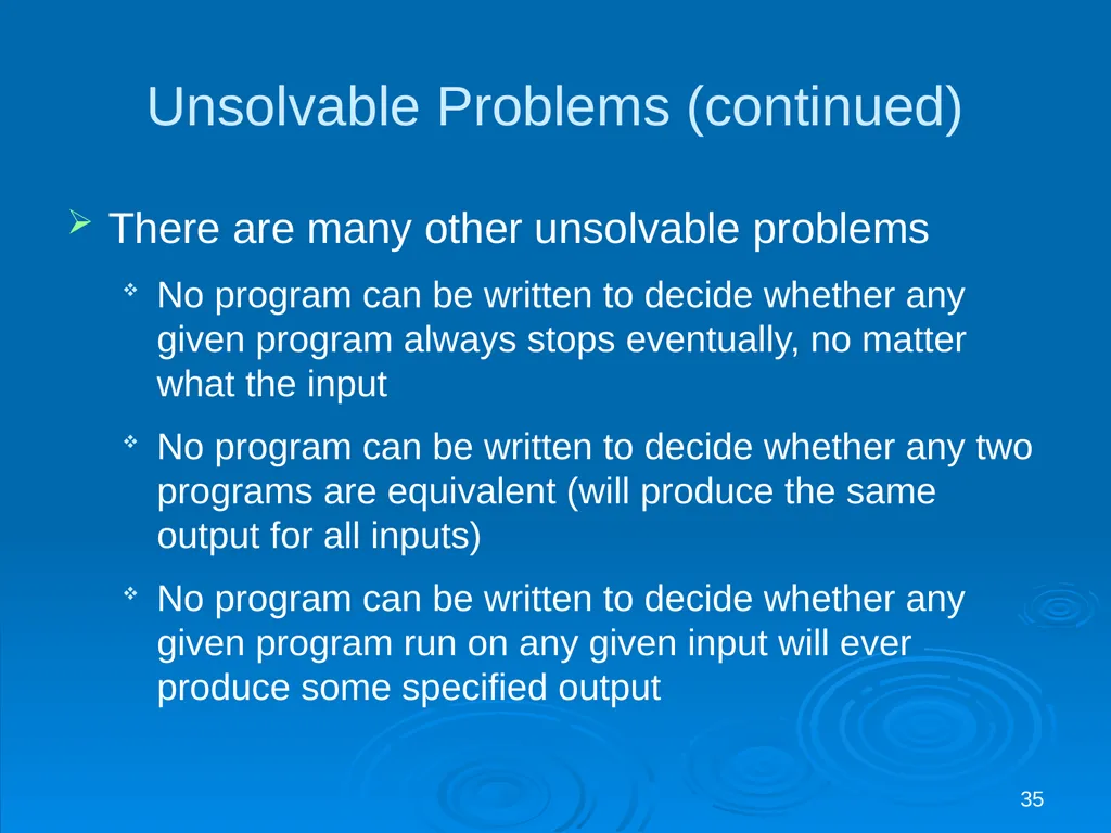
35 Unsolvable Problems (continued) There are many other unsolvable problems
No program can be written to decide whether any given program always stops eventually, no matter what the input
No program can be written to decide whether any two programs are equivalent (will produce the same output for all inputs)
No program can be written to decide whether any given program run on any given input will ever produce some specified output<br>
No program can be written to decide whether any given program always stops eventually, no matter what the input
No program can be written to decide whether any two programs are equivalent (will produce the same output for all inputs)
No program can be written to decide whether any given program run on any given input will ever produce some specified output<br>
36
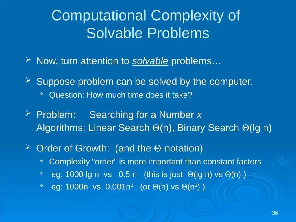
36 Computational Complexity of
Solvable Problems Now, turn attention to solvable problems…
Suppose problem can be solved by the computer.
Question: How much time does it take?
Problem: Searching for a Number x Algorithms: Linear Search (n), Binary Search (lg n)
Order of Growth: (and the -notation)
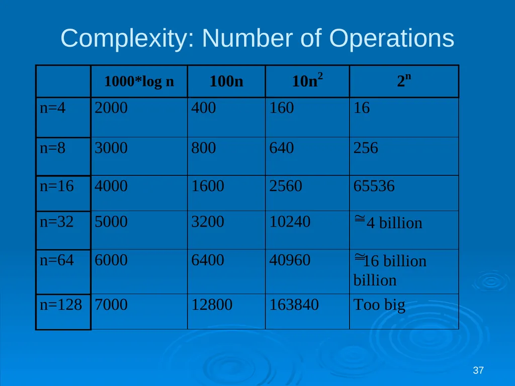
Complexity “order” is more important than constant factors
eg: 1000 lg n vs 0.5 n (this is just (lg n) vs (n) )
eg: 1000n vs 0.001n2 (or (n) vs (n2) )<br>
Suppose problem can be solved by the computer.
Question: How much time does it take?
Problem: Searching for a Number x Algorithms: Linear Search (n), Binary Search (lg n)
Order of Growth: (and the -notation)
Complexity “order” is more important than constant factors
eg: 1000 lg n vs 0.5 n (this is just (lg n) vs (n) )
eg: 1000n vs 0.001n2 (or (n) vs (n2) )<br>
37
37 Complexity: Number of Operations<br>
38
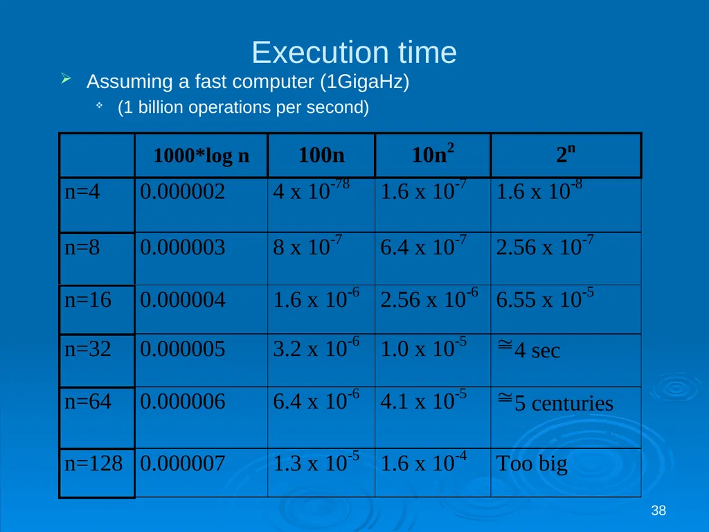
38 Execution time Assuming a fast computer (1GigaHz)
(1 billion operations per second)<br>
(1 billion operations per second)<br>
39
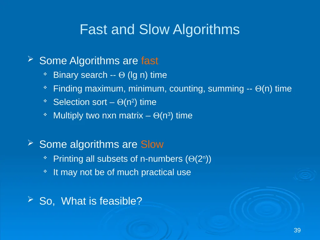
39 Fast and Slow Algorithms Some Algorithms are fast
Binary search -- (lg n) time
Finding maximum, minimum, counting, summing -- (n) time
Selection sort – (n2) time
Multiply two nxn matrix – (n3) time
Some algorithms are Slow
Printing all subsets of n-numbers ((2n))
It may not be of much practical use
So, What is feasible?<br>
Binary search -- (lg n) time
Finding maximum, minimum, counting, summing -- (n) time
Selection sort – (n2) time
Multiply two nxn matrix – (n3) time
Some algorithms are Slow
Printing all subsets of n-numbers ((2n))
It may not be of much practical use
So, What is feasible?<br>
40
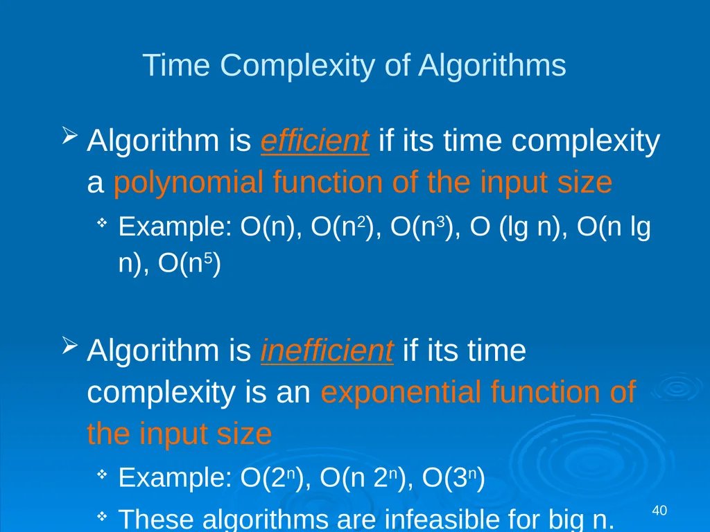
40 Time Complexity of Algorithms Algorithm is efficient if its time complexity a polynomial function of the input size
Example: O(n), O(n2), O(n3), O (lg n), O(n lg n), O(n5)
Algorithm is inefficient if its time complexity is an exponential function of the input size
Example: O(2n), O(n 2n), O(3n)
These algorithms are infeasible for big n.<br>
Example: O(n), O(n2), O(n3), O (lg n), O(n lg n), O(n5)
Algorithm is inefficient if its time complexity is an exponential function of the input size
Example: O(2n), O(n 2n), O(3n)
These algorithms are infeasible for big n.<br>
41
41 Complexity of Problems Given a problem,
can we find an efficient algorithm for it?
Yes for some problems:
Finding the maximum,
Finding the sum,
Sorting n numbers,
computing the Hamming distance
P : Class of problems that can be solved in polynomial time. (Also called easy problems)<br>
Yes for some problems:
Finding the maximum,
Finding the sum,
Sorting n numbers,
computing the Hamming distance
P : Class of problems that can be solved in polynomial time. (Also called easy problems)<br>
42
42 Remarks: The class P is invariant
under different types of machines
Turing machines, Pentium5, the world’s fastest supercomputer
Namely, if you can solve a problem B in polynomial time on a TM, then, then you can also solve B in polynomial time on supercomputer (and vice-versa)<br>
under different types of machines
Turing machines, Pentium5, the world’s fastest supercomputer
Namely, if you can solve a problem B in polynomial time on a TM, then, then you can also solve B in polynomial time on supercomputer (and vice-versa)<br>
43
43 Exponential Complexity Problems
or Hard Problems Some problems are inherently exponential time.
List all possible n-bit binary numbers;
List at 2n subsets of n objects;
List all the n! permutations of {1,2,…,n}
These are “hard problems” that require exponential time to solve.<br>
List all possible n-bit binary numbers;
List at 2n subsets of n objects;
List all the n! permutations of {1,2,…,n}
These are “hard problems” that require exponential time to solve.<br>
44
44 The Complexity class NP Given a problem, instead of finding a solution, can verify a solution to the problem quickly?
Is it easier to verify a solution (as opposed to finding a solution)
NP – the class of problems that can be verified in polynomial time<br>
Is it easier to verify a solution (as opposed to finding a solution)
NP – the class of problems that can be verified in polynomial time<br>
45
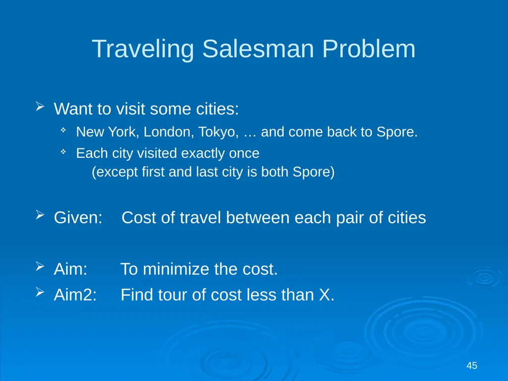
45 Want to visit some cities:
New York, London, Tokyo, … and come back to Spore.
Each city visited exactly once (except first and last city is both Spore)
Given: Cost of travel between each pair of cities
Aim: To minimize the cost.
Aim2: Find tour of cost less than X. Traveling Salesman Problem<br>
New York, London, Tokyo, … and come back to Spore.
Each city visited exactly once (except first and last city is both Spore)
Given: Cost of travel between each pair of cities
Aim: To minimize the cost.
Aim2: Find tour of cost less than X. Traveling Salesman Problem<br>
46
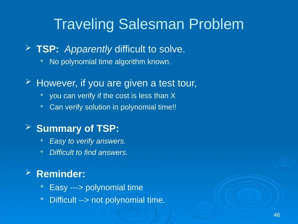
46 Traveling Salesman Problem TSP: Apparently difficult to solve.
No polynomial time algorithm known.
However, if you are given a test tour,
you can verify if the cost is less than X
Can verify solution in polynomial time!!
Summary of TSP:
Easy to verify answers.
Difficult to find answers.
Reminder:
Easy ---> polynomial time
Difficult --> not polynomial time.<br>
No polynomial time algorithm known.
However, if you are given a test tour,
you can verify if the cost is less than X
Can verify solution in polynomial time!!
Summary of TSP:
Easy to verify answers.
Difficult to find answers.
Reminder:
Easy ---> polynomial time
Difficult --> not polynomial time.<br>
47
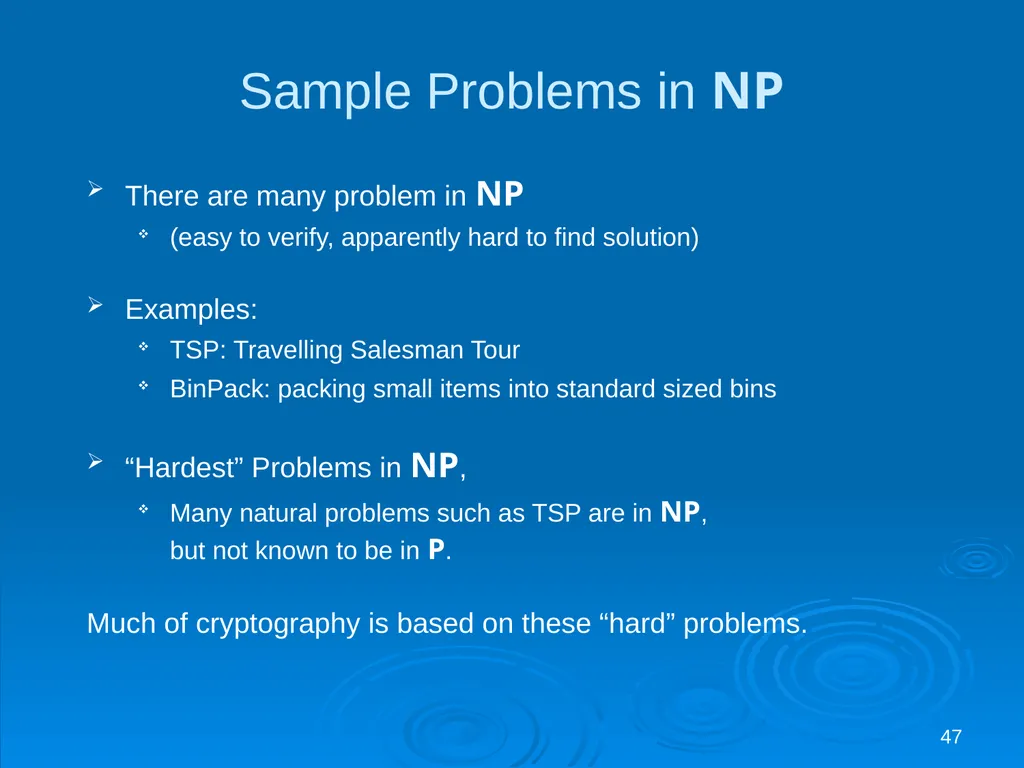
47 Sample Problems in NP There are many problem in NP
(easy to verify, apparently hard to find solution)
Examples:
TSP: Travelling Salesman Tour
BinPack: packing small items into standard sized bins
“Hardest” Problems in NP,
Many natural problems such as TSP are in NP, but not known to be in P.
Much of cryptography is based on these “hard” problems.<br>
(easy to verify, apparently hard to find solution)
Examples:
TSP: Travelling Salesman Tour
BinPack: packing small items into standard sized bins
“Hardest” Problems in NP,
Many natural problems such as TSP are in NP, but not known to be in P.
Much of cryptography is based on these “hard” problems.<br>
48
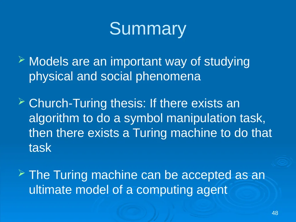
48 Summary Models are an important way of studying physical and social phenomena
Church-Turing thesis: If there exists an algorithm to do a symbol manipulation task, then there exists a Turing machine to do that task
The Turing machine can be accepted as an ultimate model of a computing agent<br>
Church-Turing thesis: If there exists an algorithm to do a symbol manipulation task, then there exists a Turing machine to do that task
The Turing machine can be accepted as an ultimate model of a computing agent<br>
49
49 Summary (continued) A Turing machine program can be accepted as an ultimate model of an algorithm
Turing machines define the limits of computability
An uncomputable or unsolvable problem: We can prove that no Turing machine exists to solve the problem<br>
Turing machines define the limits of computability
An uncomputable or unsolvable problem: We can prove that no Turing machine exists to solve the problem<br>
50
50 The End…<br>