
A CFD-to-Radiation Framework for Line-by- Line
LD
Published · 20 slides · 0 views

1 / 1




Description
A CFD-to-Radiation Framework for Line-by- Line Infrared Emission Modelling of High- Temperature Exhaust Plumes Salvatore Esposito Italian Aerospace Research Centre Luigi Cutrone Italian Aerospace Research Centre Antonio Schettino -
Related Topics
Share
Embed code
Download this presentation From Below
"A CFD-to-Radiation Framework for Line-by- Line" is the property of its rightful owner. Permission is granted to download and print the materials on this website for personal, non-commercial use only, and to display it on your personal computer provided you do not modify the materials and that you retain all copyright notices contained in the materials. By downloading content from our website, you accept the terms of this agreement.
Presentation Transcript
01
A CFD-to-Radiation Framework for Line-by-
Line Infrared Emission Modelling of High-
Temperature Exhaust Plumes Salvatore Esposito – Italian Aerospace Research Centre Luigi Cutrone – Italian Aerospace Research Centre Antonio Schettino - Italian Aerospace Research Centre ◎ 11ᵗʰ International Workshop on Radiation of
High Temperature Gases for Space Missions
Mola di Bari, 21–25 September 2026<br>
Line Infrared Emission Modelling of High-
Temperature Exhaust Plumes Salvatore Esposito – Italian Aerospace Research Centre Luigi Cutrone – Italian Aerospace Research Centre Antonio Schettino - Italian Aerospace Research Centre ◎ 11ᵗʰ International Workshop on Radiation of
High Temperature Gases for Space Missions
Mola di Bari, 21–25 September 2026<br>
02
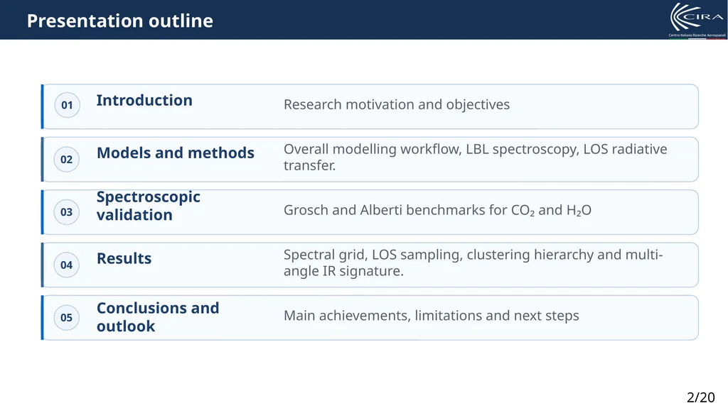
Introduction Research motivation and objectives 02 Models and methods Overall modelling workflow, LBL spectroscopy, LOS radiative transfer. 03 Spectroscopic validation Grosch and Alberti benchmarks for CO₂ and H₂O 04 Results Spectral grid, LOS sampling, clustering hierarchy and multi-angle IR signature. 05 Conclusions and outlook Main achievements, limitations and next steps Presentation outline 01 2/20<br>
03
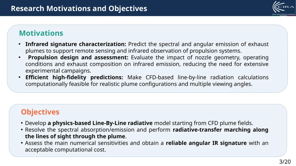
Research Motivations and Objectives 3/20<br>
04
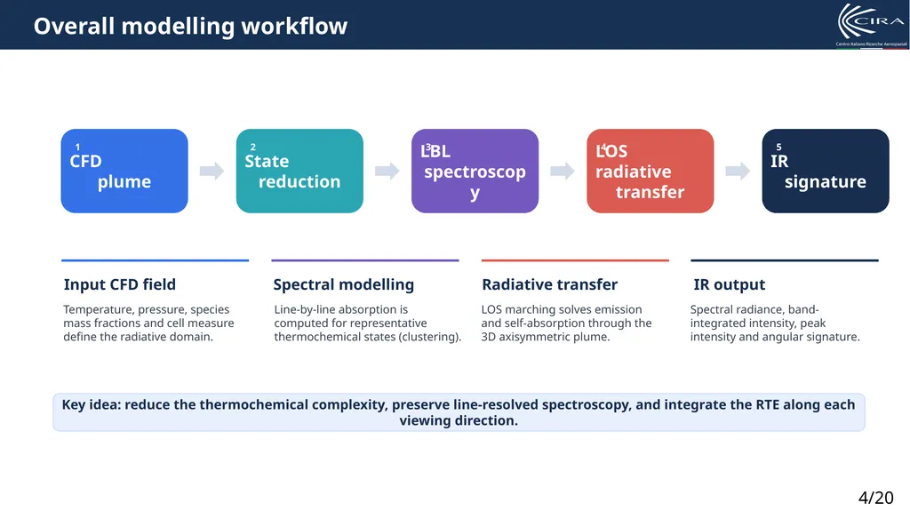
CFD
plume 1 State
reduction 2 LBL
spectroscopy 3 LOS radiative
transfer 4 IR
signature 5 Input CFD field Temperature, pressure, species
mass fractions and cell measure
define the radiative domain. Spectral modelling Line-by-line absorption is
computed for representative
thermochemical states (clustering). Radiative transfer LOS marching solves emission
and self-absorption through the
3D axisymmetric plume. IR output Spectral radiance, band-
integrated intensity, peak
intensity and angular signature. Key idea: reduce the thermochemical complexity, preserve line-resolved spectroscopy, and integrate the RTE along each viewing direction. Overall modelling workflow 4/20<br>
plume 1 State
reduction 2 LBL
spectroscopy 3 LOS radiative
transfer 4 IR
signature 5 Input CFD field Temperature, pressure, species
mass fractions and cell measure
define the radiative domain. Spectral modelling Line-by-line absorption is
computed for representative
thermochemical states (clustering). Radiative transfer LOS marching solves emission
and self-absorption through the
3D axisymmetric plume. IR output Spectral radiance, band-
integrated intensity, peak
intensity and angular signature. Key idea: reduce the thermochemical complexity, preserve line-resolved spectroscopy, and integrate the RTE along each viewing direction. Overall modelling workflow 4/20<br>
05
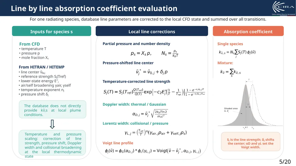
For one radiating species, database line parameters are corrected to the local CFD state and summed over all transitions. Local line corrections Partial pressure and number density Pressure-shifted line center Temperature-corrected line strength Doppler width: thermal / Gaussian Lorentz width: collisional / pressure Voigt line profile Absorption coefficient Sⱼ is the line strength; δⱼ shifts the center; αD and γL set the Voigt width. Single species Mixture: Temperature and pressure scaling: correction of line strength, pressure shift, Doppler width and collisional broadening at the local thermodynamic state Line by line absorption coefficient evaluation 5/20<br>
06
Line-of-sight radiative marching For each viewing angle, each ray is marched cell-by-cell from the far side of the plume toward the observer. Marching along one ray 1 Trace LOS camera plane → ordered ray/cell intersections 2 Build segments for each crossed cell i: Δsᵢ, Tᵢ, pᵢ, Xᵢ 3 Optical depth τν̃,ᵢ = kν̃,ᵢ Δsᵢ [-] 4 Radiance update attenuation + local Planck emission Segment solution uniform kν̃ and T only inside segment i Ray bundle and plume sampling Each ray crosses a different ordered sequence of cells and samples the local LBL properties along its path. From marched rays to angular band intensity Lν̃,r [W m⁻² sr⁻¹ (cm⁻¹)⁻¹] Lr,band [W m⁻² sr⁻¹] I r,band [W sr⁻¹] Iband(θ) [W sr⁻¹] Area weight wᵣ = Aᵣ is the camera-plane area represented by ray r [m²]. far side cell 1 cell 2 cell 3 cell 4 6/20 camera<br>
07
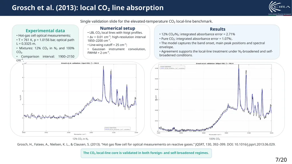
Grosch et al. (2013): local CO₂ line absorption Single validation slide for the elevated-temperature CO₂ local-line benchmark. Experimental data • Hot-gas cell optical measurements;
• T = 761 K, p = 1.0156 bar, optical path L = 0.3325 m.
• Mixtures: 12% CO₂ in N₂ and 100% CO₂.
• Comparison interval: 1900–2150 cm⁻¹. Numerical setup • LBL CO₂ local lines with Voigt profiles.
• Δν = 0.01 cm⁻¹; high-resolution interval 1850–2200 cm⁻¹.
• Line-wing cutoff = 25 cm⁻¹;
• Gaussian instrument convolution, FWHM = 2 cm⁻¹. Results • 12% CO₂/N₂: integrated absorbance error = 2.71%
• Pure CO₂: integrated absorbance error = 1.07%;.
• The model captures the band onset, main peak positions and spectral envelope.
• Agreement supports the local-line treatment under N₂-broadened and self-broadened conditions. 12% CO₂ in N₂ 100% CO₂ The CO₂ local-line core is validated in both foreign- and self-broadened regimes. Grosch, H., Fateev, A., Nielsen, K. L., & Clausen, S. (2013). “Hot gas flow cell for optical measurements on reactive gases.” JQSRT, 130, 392–399. DOI: 10.1016/j.jqsrt.2013.06.029. 7/20<br>
• T = 761 K, p = 1.0156 bar, optical path L = 0.3325 m.
• Mixtures: 12% CO₂ in N₂ and 100% CO₂.
• Comparison interval: 1900–2150 cm⁻¹. Numerical setup • LBL CO₂ local lines with Voigt profiles.
• Δν = 0.01 cm⁻¹; high-resolution interval 1850–2200 cm⁻¹.
• Line-wing cutoff = 25 cm⁻¹;
• Gaussian instrument convolution, FWHM = 2 cm⁻¹. Results • 12% CO₂/N₂: integrated absorbance error = 2.71%
• Pure CO₂: integrated absorbance error = 1.07%;.
• The model captures the band onset, main peak positions and spectral envelope.
• Agreement supports the local-line treatment under N₂-broadened and self-broadened conditions. 12% CO₂ in N₂ 100% CO₂ The CO₂ local-line core is validated in both foreign- and self-broadened regimes. Grosch, H., Fateev, A., Nielsen, K. L., & Clausen, S. (2013). “Hot gas flow cell for optical measurements on reactive gases.” JQSRT, 130, 392–399. DOI: 10.1016/j.jqsrt.2013.06.029. 7/20<br>
08
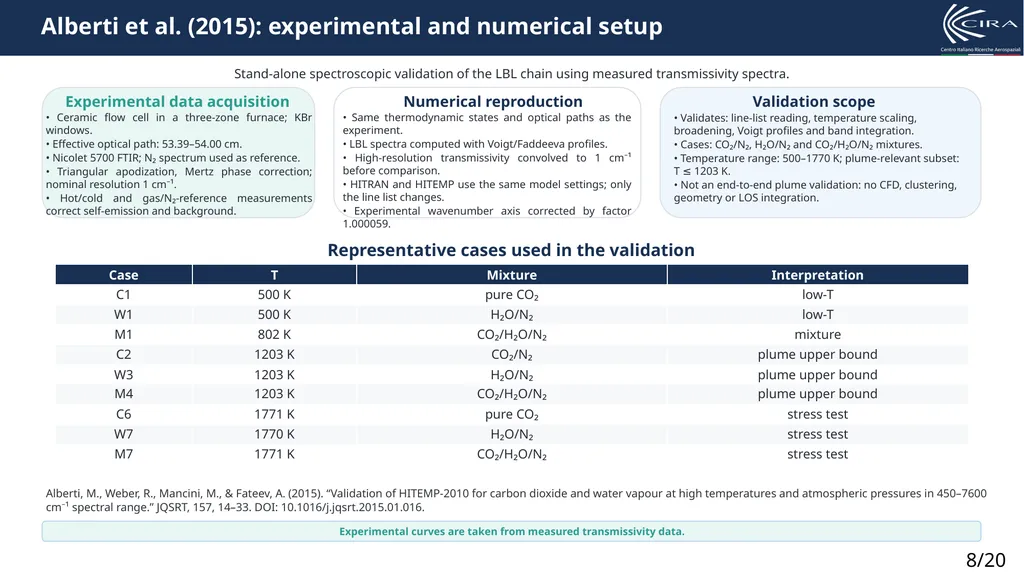
Alberti et al. (2015): experimental and numerical setup Stand-alone spectroscopic validation of the LBL chain using measured transmissivity spectra. Experimental data acquisition • Ceramic flow cell in a three-zone furnace; KBr windows.
• Effective optical path: 53.39–54.00 cm.
• Nicolet 5700 FTIR; N₂ spectrum used as reference.
• Triangular apodization, Mertz phase correction; nominal resolution 1 cm⁻¹.
• Hot/cold and gas/N₂-reference measurements correct self-emission and background. Numerical reproduction • Same thermodynamic states and optical paths as the experiment.
• LBL spectra computed with Voigt/Faddeeva profiles.
• High-resolution transmissivity convolved to 1 cm⁻¹ before comparison.
• HITRAN and HITEMP use the same model settings; only the line list changes.
• Experimental wavenumber axis corrected by factor 1.000059. Validation scope • Validates: line-list reading, temperature scaling, broadening, Voigt profiles and band integration.
• Cases: CO₂/N₂, H₂O/N₂ and CO₂/H₂O/N₂ mixtures.
• Temperature range: 500–1770 K; plume-relevant subset: T ≤ 1203 K.
• Not an end-to-end plume validation: no CFD, clustering, geometry or LOS integration. Representative cases used in the validation Experimental curves are taken from measured transmissivity data. Alberti, M., Weber, R., Mancini, M., & Fateev, A. (2015). “Validation of HITEMP-2010 for carbon dioxide and water vapour at high temperatures and atmospheric pressures in 450–7600 cm⁻¹ spectral range.” JQSRT, 157, 14–33. DOI: 10.1016/j.jqsrt.2015.01.016. 8/20<br>
• Effective optical path: 53.39–54.00 cm.
• Nicolet 5700 FTIR; N₂ spectrum used as reference.
• Triangular apodization, Mertz phase correction; nominal resolution 1 cm⁻¹.
• Hot/cold and gas/N₂-reference measurements correct self-emission and background. Numerical reproduction • Same thermodynamic states and optical paths as the experiment.
• LBL spectra computed with Voigt/Faddeeva profiles.
• High-resolution transmissivity convolved to 1 cm⁻¹ before comparison.
• HITRAN and HITEMP use the same model settings; only the line list changes.
• Experimental wavenumber axis corrected by factor 1.000059. Validation scope • Validates: line-list reading, temperature scaling, broadening, Voigt profiles and band integration.
• Cases: CO₂/N₂, H₂O/N₂ and CO₂/H₂O/N₂ mixtures.
• Temperature range: 500–1770 K; plume-relevant subset: T ≤ 1203 K.
• Not an end-to-end plume validation: no CFD, clustering, geometry or LOS integration. Representative cases used in the validation Experimental curves are taken from measured transmissivity data. Alberti, M., Weber, R., Mancini, M., & Fateev, A. (2015). “Validation of HITEMP-2010 for carbon dioxide and water vapour at high temperatures and atmospheric pressures in 450–7600 cm⁻¹ spectral range.” JQSRT, 157, 14–33. DOI: 10.1016/j.jqsrt.2015.01.016. 8/20<br>
09
Alberti results: HITRAN–HITEMP comparison Aggregate behaviour over 54 case-band combinations and over the plume-relevant temperature subset. Mean RMSE 0.089 → 0.056 HITRAN to HITEMP; −37% Mean |ε| error 13.9% → 9.6% all cases; −30% T ≤ 1203 K RMSE 0.055 → 0.046 plume-relevant; −16% T ≤ 1203 K |ε| 7.8% → 6.7% plume-relevant; −14% Band-by-band outcome 19 vs 17 HITRAN lower RMSE in 19 cases; HITEMP in 17, for T≤1203 K HITEMP improves the aggregate statistics, but within the plume range the advantage is moderate and band-dependent. 9/20<br>
10
Alberti results within the plume temperature envelope Cases up to approximately 1200 K are the most relevant subset for the present plume calculations. Case-averaged quantitative indicators Main message: up to 1200 K, HITEMP is better on average, but not uniformly superior in every band. 10/20<br>
11
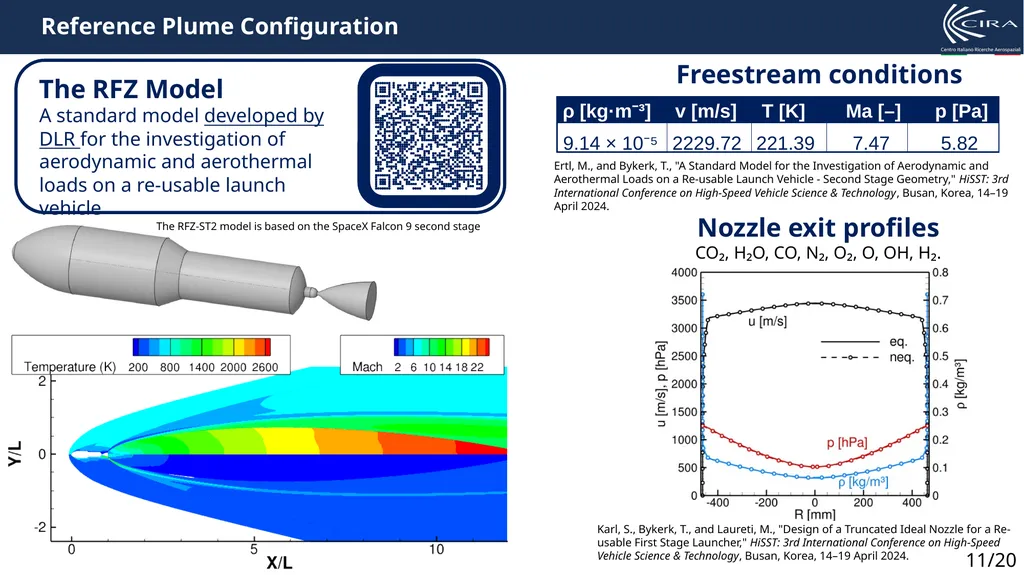
The RFZ Model
A standard model developed by DLR for the investigation of aerodynamic and aerothermal loads on a re-usable launch vehicle The RFZ-ST2 model is based on the SpaceX Falcon 9 second stage Nozzle exit profiles
CO₂, H₂O, CO, N₂, O₂, O, OH, H₂. Freestream conditions Karl, S., Bykerk, T., and Laureti, M., "Design of a Truncated Ideal Nozzle for a Re-usable First Stage Launcher," HiSST: 3rd International Conference on High-Speed Vehicle Science & Technology, Busan, Korea, 14–19 April 2024. Ertl, M., and Bykerk, T., "A Standard Model for the Investigation of Aerodynamic and Aerothermal Loads on a Re-usable Launch Vehicle - Second Stage Geometry," HiSST: 3rd International Conference on High-Speed Vehicle Science & Technology, Busan, Korea, 14–19 April 2024. Reference Plume Configuration 11/20<br>
A standard model developed by DLR for the investigation of aerodynamic and aerothermal loads on a re-usable launch vehicle The RFZ-ST2 model is based on the SpaceX Falcon 9 second stage Nozzle exit profiles
CO₂, H₂O, CO, N₂, O₂, O, OH, H₂. Freestream conditions Karl, S., Bykerk, T., and Laureti, M., "Design of a Truncated Ideal Nozzle for a Re-usable First Stage Launcher," HiSST: 3rd International Conference on High-Speed Vehicle Science & Technology, Busan, Korea, 14–19 April 2024. Ertl, M., and Bykerk, T., "A Standard Model for the Investigation of Aerodynamic and Aerothermal Loads on a Re-usable Launch Vehicle - Second Stage Geometry," HiSST: 3rd International Conference on High-Speed Vehicle Science & Technology, Busan, Korea, 14–19 April 2024. Reference Plume Configuration 11/20<br>
12
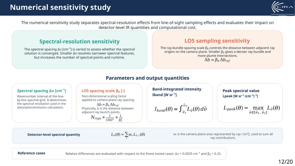
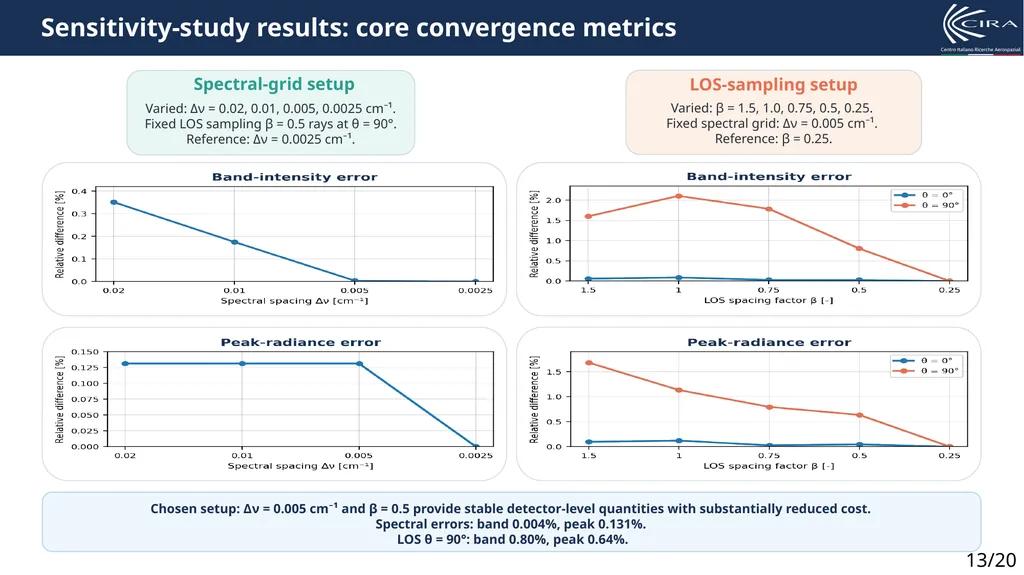
Numerical sensitivity study The numerical sensitivity study separates spectral-resolution effects from line-of-sight sampling effects and evaluates their impact on detector-level IR quantities and computational cost. Spectral-resolution sensitivity The spectral spacing Δν [cm⁻¹] is varied to assess whether the spectral solution is converged. Smaller Δν resolves narrower spectral features, but increases the number of spectral points and runtime. LOS sampling sensitivity The ray-bundle spacing scale βᵦ controls the distance between adjacent ray origins on the camera plane. Smaller βᵦ gives a denser ray bundle and more plume intersections. Parameters and output quantities Spectral spacing Δν [cm⁻¹] Wavenumber interval of the line-by-line spectral grid. It determines the spectral resolution used in the absorption/emission calculation. LOS spacing scale βᵦ [-] Non-dimensional scaling factor applied to camera-plane ray spacing: Physically, b is the distance between adjacent ray launch points. Band-integrated intensity Iband [W sr⁻¹] Peak spectral value Lpeak [W sr⁻¹ (cm⁻¹)⁻¹] Detector-level spectral quantity wᵣ is the camera-plane area represented by ray r [m²], used to sum all ray contributions. Reference cases Relative differences are evaluated with respect to the finest tested cases: Δν = 0.0025 cm⁻¹ and βᵦ = 0.25. 12/20<br>
13
Sensitivity-study results: core convergence metrics Spectral-grid setup Varied: Δν = 0.02, 0.01, 0.005, 0.0025 cm⁻¹.
Fixed LOS sampling β = 0.5 rays at θ = 90°. Reference: Δν = 0.0025 cm⁻¹. LOS-sampling setup Varied: β = 1.5, 1.0, 0.75, 0.5, 0.25.
Fixed spectral grid: Δν = 0.005 cm⁻¹.
Reference: β = 0.25. Chosen setup: Δν = 0.005 cm⁻¹ and β = 0.5 provide stable detector-level quantities with substantially reduced cost.
Spectral errors: band 0.004%, peak 0.131%.
LOS θ = 90°: band 0.80%, peak 0.64%. 13/20<br>
Fixed LOS sampling β = 0.5 rays at θ = 90°. Reference: Δν = 0.0025 cm⁻¹. LOS-sampling setup Varied: β = 1.5, 1.0, 0.75, 0.5, 0.25.
Fixed spectral grid: Δν = 0.005 cm⁻¹.
Reference: β = 0.25. Chosen setup: Δν = 0.005 cm⁻¹ and β = 0.5 provide stable detector-level quantities with substantially reduced cost.
Spectral errors: band 0.004%, peak 0.131%.
LOS θ = 90°: band 0.80%, peak 0.64%. 13/20<br>
14
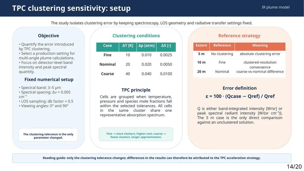
TPC clustering sensitivity: setup IR plume model The study isolates clustering error by keeping spectroscopy, LOS geometry and radiative transfer settings fixed. Objective • Quantify the error introduced by TPC clustering.
• Select a production setting for multi-angle plume calculations.
• Focus on detector-level band intensity and peak spectral quantity. Fixed numerical setup • Spectral band: 3–5 μm
• Spectral spacing: Δν = 0.005 cm⁻¹
• LOS sampling: db factor = 0.5
• Viewing angles: 0° and 90° The clustering tolerance is the only parameter changed. Clustering conditions TPC principle Cells are grouped when temperature, pressure and species mole fractions fall within the selected tolerances. All cells in the same cluster share one representative absorption spectrum. Fine → more clusters, higher cost; coarse → fewer clusters, larger approximation. Reference strategy Error definition ε = 100 · (Qcase − Qref) / Qref Q is either band-integrated intensity [W/sr] or peak spectral radiant intensity [W/(sr cm⁻¹)]. The 5 m case is the only direct comparison against an unclustered solution. Reading guide: only the clustering tolerance changes; differences in the results can therefore be attributed to the TPC acceleration strategy. 14/20<br>
• Select a production setting for multi-angle plume calculations.
• Focus on detector-level band intensity and peak spectral quantity. Fixed numerical setup • Spectral band: 3–5 μm
• Spectral spacing: Δν = 0.005 cm⁻¹
• LOS sampling: db factor = 0.5
• Viewing angles: 0° and 90° The clustering tolerance is the only parameter changed. Clustering conditions TPC principle Cells are grouped when temperature, pressure and species mole fractions fall within the selected tolerances. All cells in the same cluster share one representative absorption spectrum. Fine → more clusters, higher cost; coarse → fewer clusters, larger approximation. Reference strategy Error definition ε = 100 · (Qcase − Qref) / Qref Q is either band-integrated intensity [W/sr] or peak spectral radiant intensity [W/(sr cm⁻¹)]. The 5 m case is the only direct comparison against an unclustered solution. Reading guide: only the clustering tolerance changes; differences in the results can therefore be attributed to the TPC acceleration strategy. 14/20<br>
15
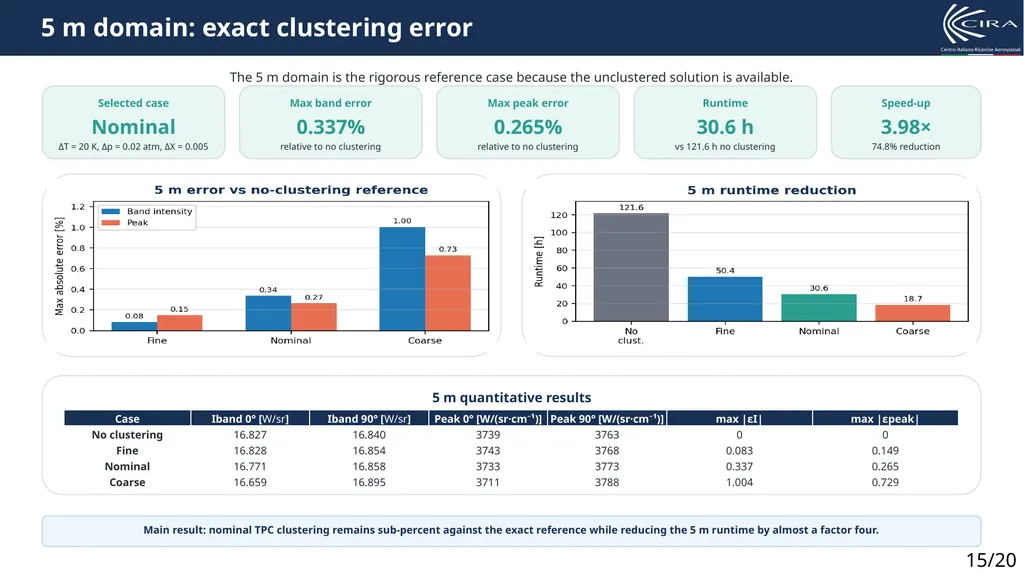
5 m domain: exact clustering error The 5 m domain is the rigorous reference case because the unclustered solution is available. Selected case Nominal ΔT = 20 K, Δp = 0.02 atm, ΔX = 0.005 Max band error 0.337% relative to no clustering Max peak error 0.265% relative to no clustering Runtime 30.6 h vs 121.6 h no clustering Speed-up 3.98× 74.8% reduction 5 m quantitative results Main result: nominal TPC clustering remains sub-percent against the exact reference while reducing the 5 m runtime by almost a factor four. 15/20<br>
16
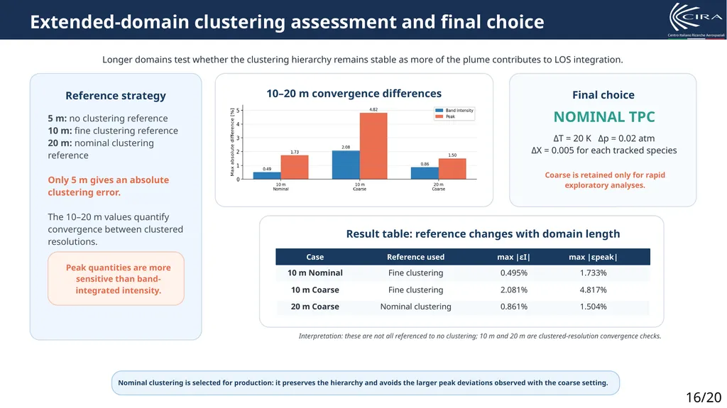
Extended-domain clustering assessment and final choice Reference strategy 5 m: no clustering reference
10 m: fine clustering reference
20 m: nominal clustering reference
Only 5 m gives an absolute clustering error.
The 10–20 m values quantify convergence between clustered resolutions. Peak quantities are more sensitive than band-integrated intensity. 10–20 m convergence differences Final choice NOMINAL TPC ΔT = 20 K Δp = 0.02 atm
ΔX = 0.005 for each tracked species Coarse is retained only for rapid exploratory analyses. Nominal clustering is selected for production: it preserves the hierarchy and avoids the larger peak deviations observed with the coarse setting. Longer domains test whether the clustering hierarchy remains stable as more of the plume contributes to LOS integration. 16/20<br>
10 m: fine clustering reference
20 m: nominal clustering reference
Only 5 m gives an absolute clustering error.
The 10–20 m values quantify convergence between clustered resolutions. Peak quantities are more sensitive than band-integrated intensity. 10–20 m convergence differences Final choice NOMINAL TPC ΔT = 20 K Δp = 0.02 atm
ΔX = 0.005 for each tracked species Coarse is retained only for rapid exploratory analyses. Nominal clustering is selected for production: it preserves the hierarchy and avoids the larger peak deviations observed with the coarse setting. Longer domains test whether the clustering hierarchy remains stable as more of the plume contributes to LOS integration. 16/20<br>
17
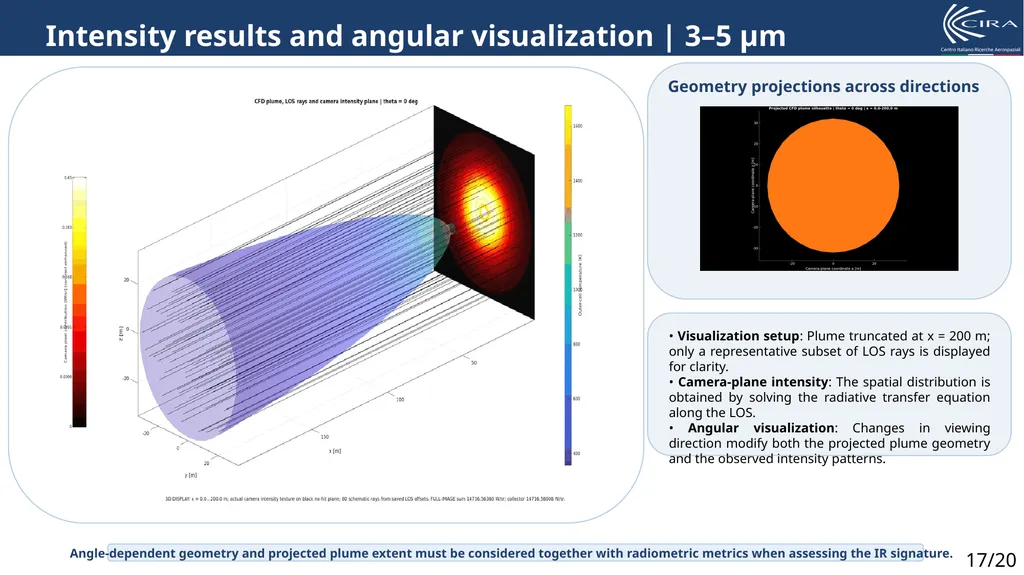
Intensity results and angular visualization | 3–5 µm Angle-dependent geometry and projected plume extent must be considered together with radiometric metrics when assessing the IR signature. • Visualization setup: Plume truncated at x = 200 m; only a representative subset of LOS rays is displayed for clarity.
• Camera-plane intensity: The spatial distribution is obtained by solving the radiative transfer equation along the LOS.
• Angular visualization: Changes in viewing direction modify both the projected plume geometry and the observed intensity patterns. 17/20<br>
• Camera-plane intensity: The spatial distribution is obtained by solving the radiative transfer equation along the LOS.
• Angular visualization: Changes in viewing direction modify both the projected plume geometry and the observed intensity patterns. 17/20<br>
18
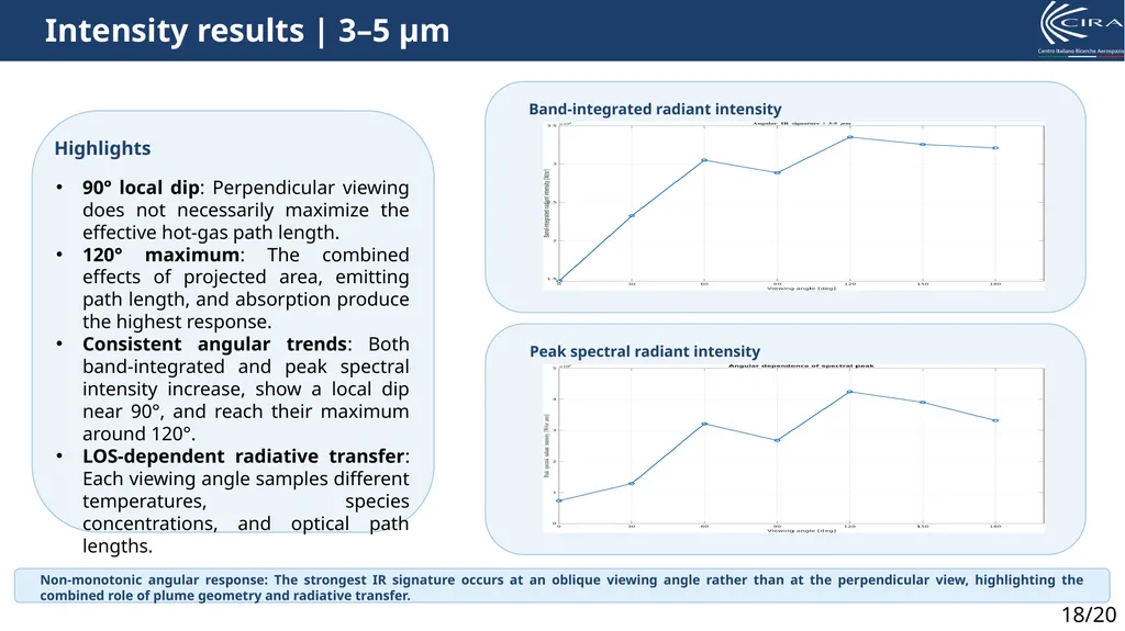
Angular dependence and physical interpretation | 3–5 μm Non-monotonic angular response: The strongest IR signature occurs at an oblique viewing angle rather than at the perpendicular view, highlighting the combined role of plume geometry and radiative transfer. Intensity results | 3–5 µm 18/20<br>
19
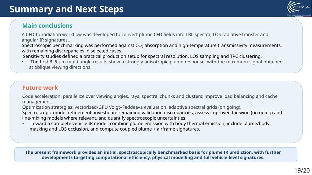
Summary and Next Steps The present framework provides an initial, spectroscopically benchmarked basis for plume IR prediction, with further developments targeting computational efficiency, physical modelling and full vehicle-level signatures. 19/20<br>
20
Bibliography 20/20<br>