04
Motivation Problem: Localization
GPS is unreliable or unavailable in some environments
Inertial Measurement Units (IMUs) and cameras are small, inexpensive, and have low power consumption
Fused IMU and camera measurements can provide very accurate pose estimates<br>
05
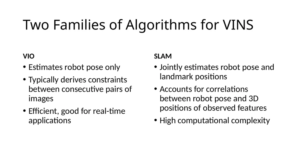
Two Families of Algorithms for VINS VIO Estimates robot pose only
Typically derives constraints between consecutive pairs of images
Efficient, good for real-time applications SLAM Jointly estimates robot pose and landmark positions
Accounts for correlations between robot pose and 3D positions of observed features
High computational complexity<br>
06
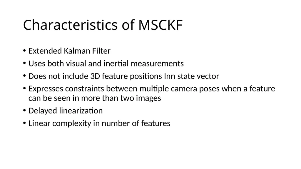
Characteristics of MSCKF Extended Kalman Filter
Uses both visual and inertial measurements
Does not include 3D feature positions Inn state vector
Expresses constraints between multiple camera poses when a feature can be seen in more than two images
Delayed linearization
Linear complexity in number of features<br>
08
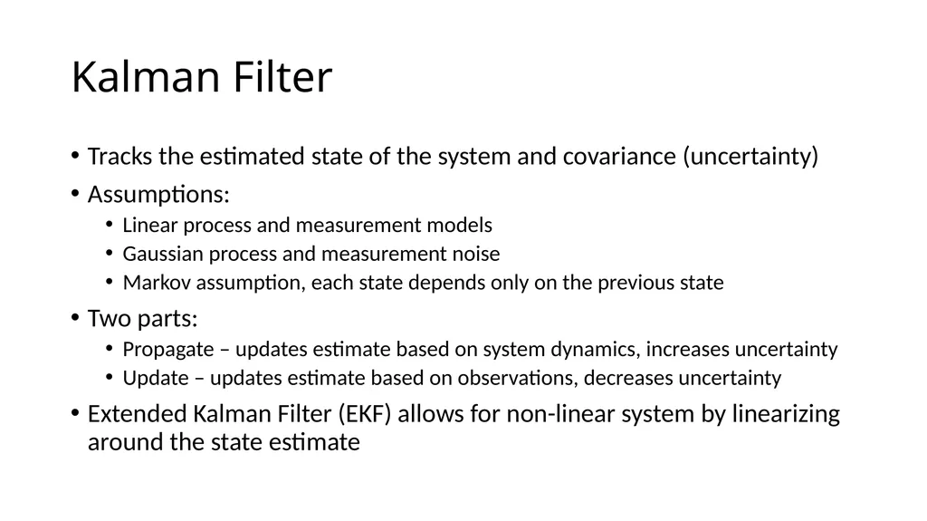
Kalman Filter Tracks the estimated state of the system and covariance (uncertainty)
Assumptions:
Linear process and measurement models
Gaussian process and measurement noise
Markov assumption, each state depends only on the previous state
Two parts:
Propagate – updates estimate based on system dynamics, increases uncertainty
Update – updates estimate based on observations, decreases uncertainty
Extended Kalman Filter (EKF) allows for non-linear system by linearizing around the state estimate<br>
09
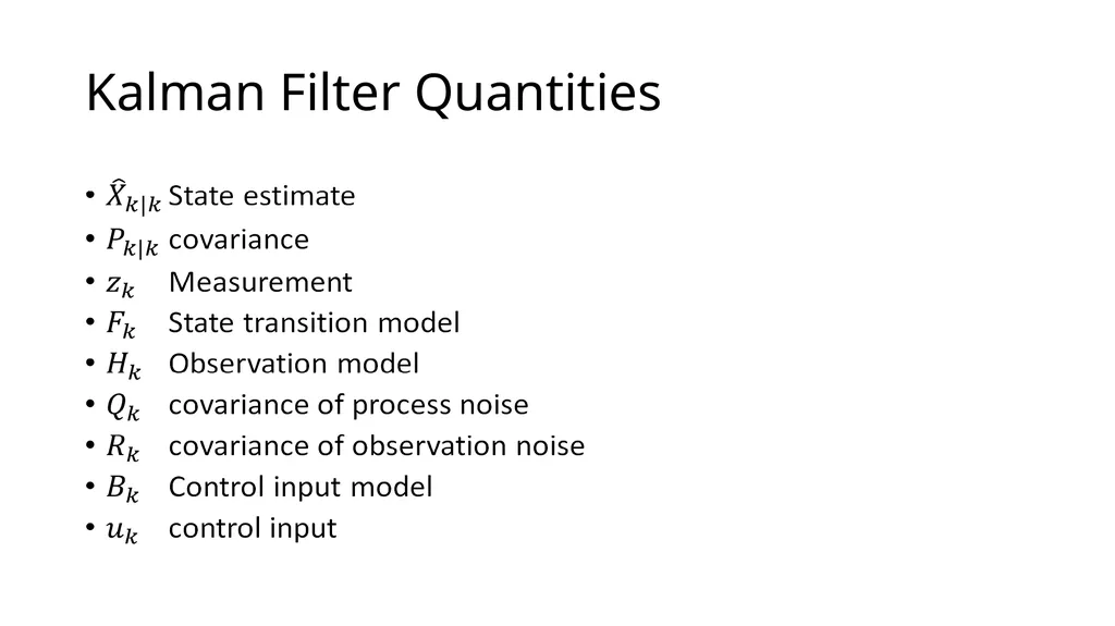
Kalman Filter Quantities<br>
10
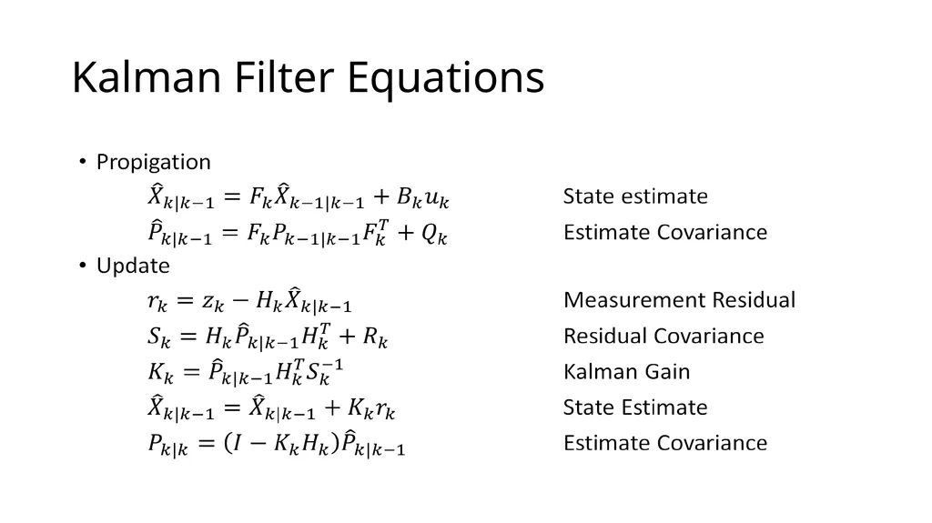
Kalman Filter Equations<br>
11
MSCKF Estimator Description<br>
13
Frames of Reference Goal of MSCKF is to track the 3D pose of the IMU affixed frame {I} with respect to the global frame {G}
{G} is an Earth-centered, Earth-fixed frame to simplify effects of Earth’s rotation on IMU measurements<br>
14
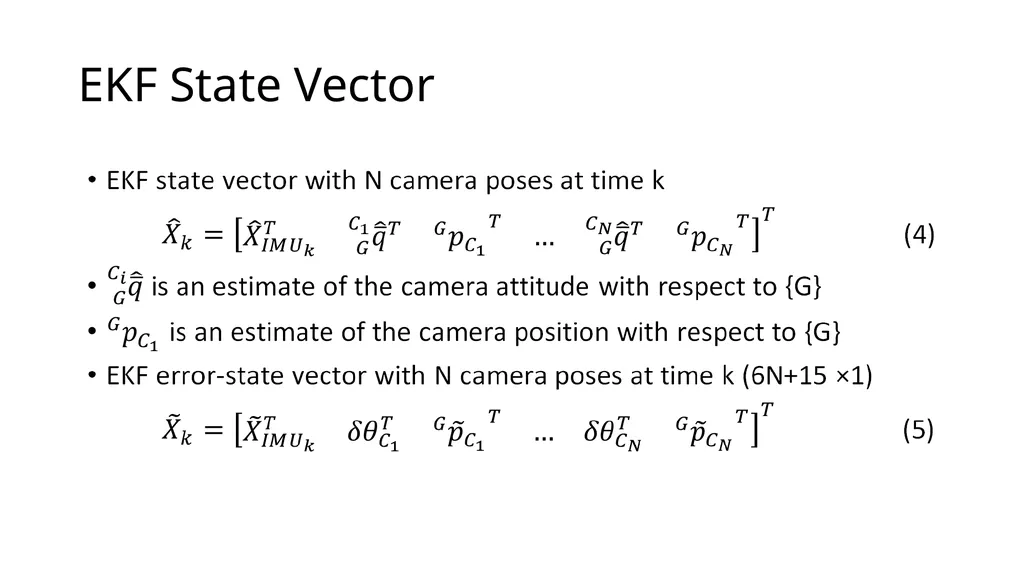
MSCKF Algorithm Propagation: For each IMU measurement received, propagate the filter state and covariance.
Image registration: Every time a new image is recorded,
augment the state vector and covariance matrix with a copy of the current camera pose estimate.
image processing module begins operation.
Update: When the feature measurements of a given image become available, perform an EKF update.<br>
17
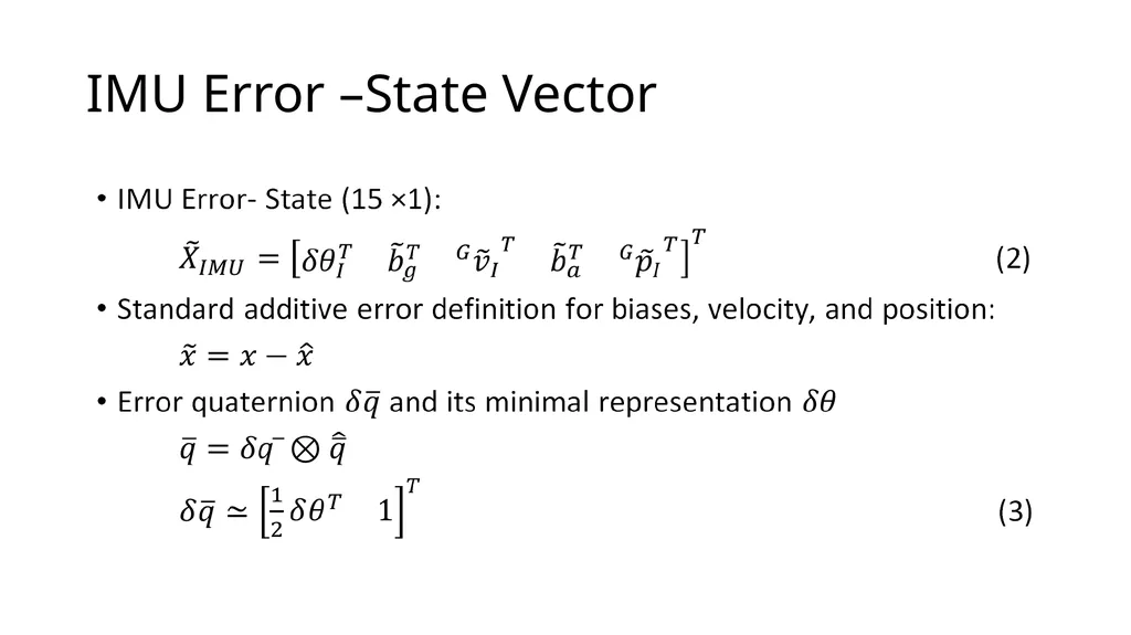
IMU Error –State Vector<br>
20
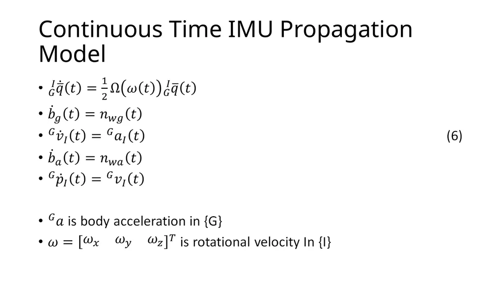
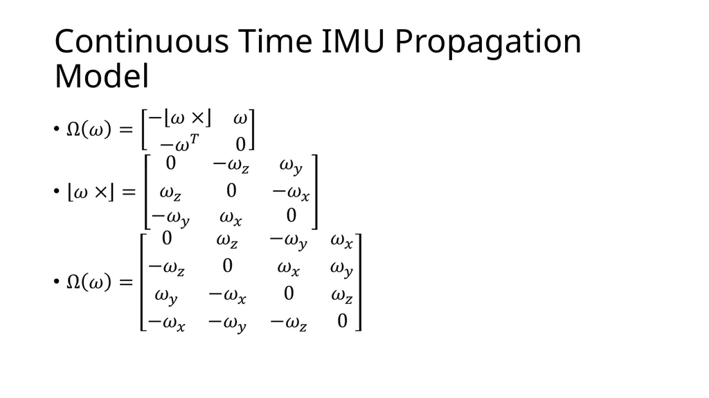
Continuous Time IMU Propagation Model<br>
21
Continuous Time IMU Propagation Model<br>
22
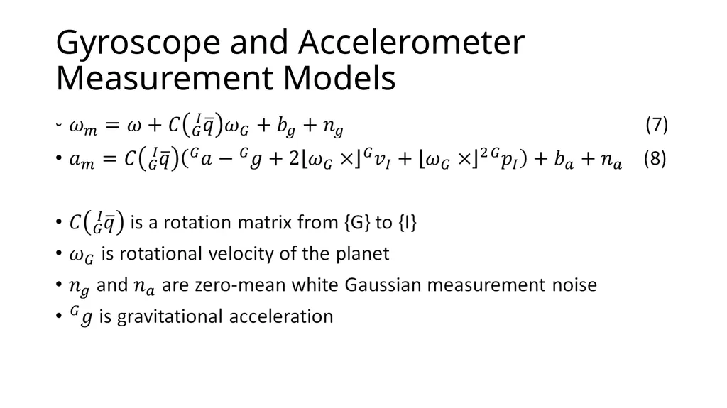
Gyroscope and Accelerometer Measurement Models<br>
23
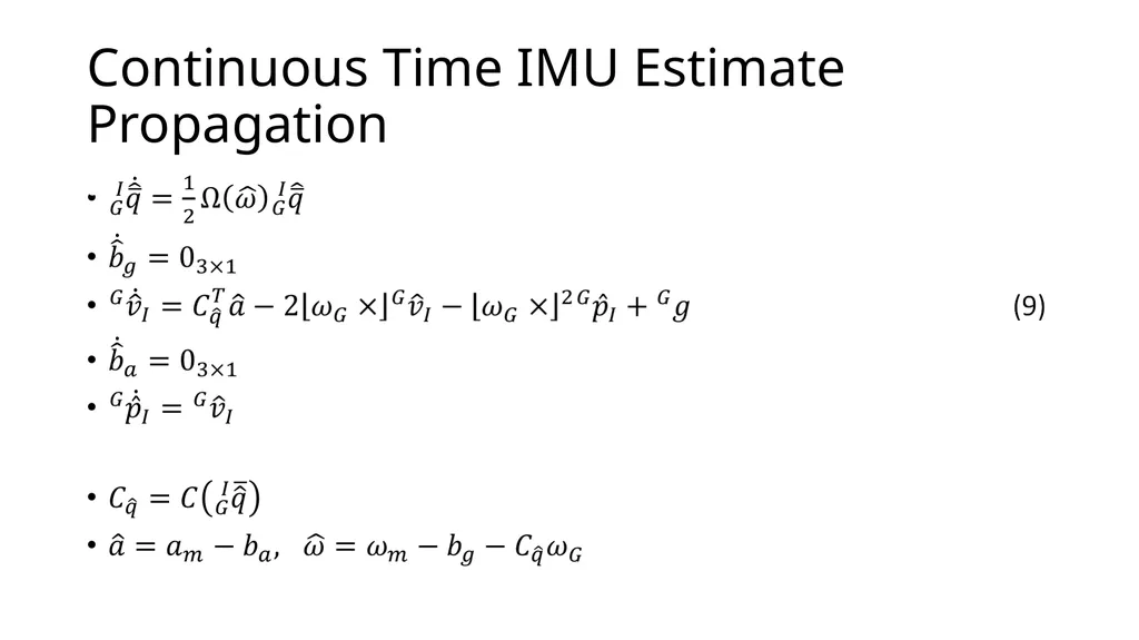
Continuous Time IMU Estimate Propagation<br>
24
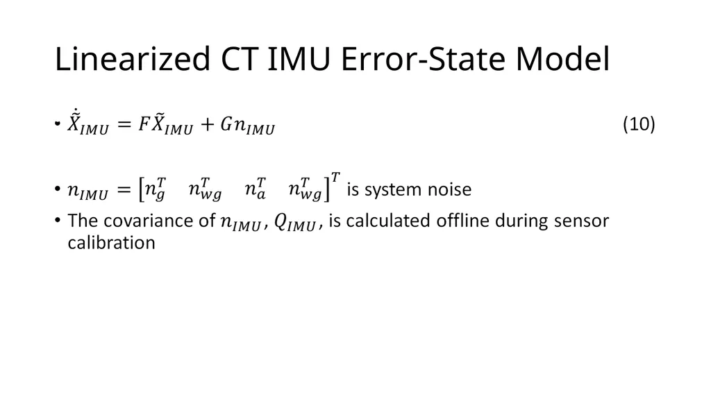
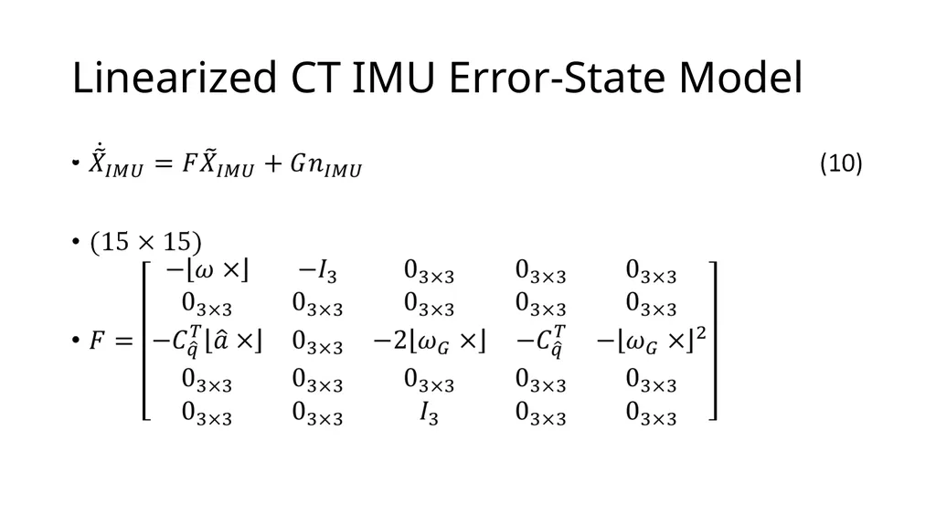
Linearized CT IMU Error-State Model<br>
25
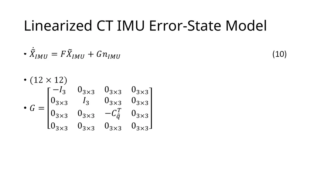
Linearized CT IMU Error-State Model<br>
26
Linearized CT IMU Error-State Model<br>
27
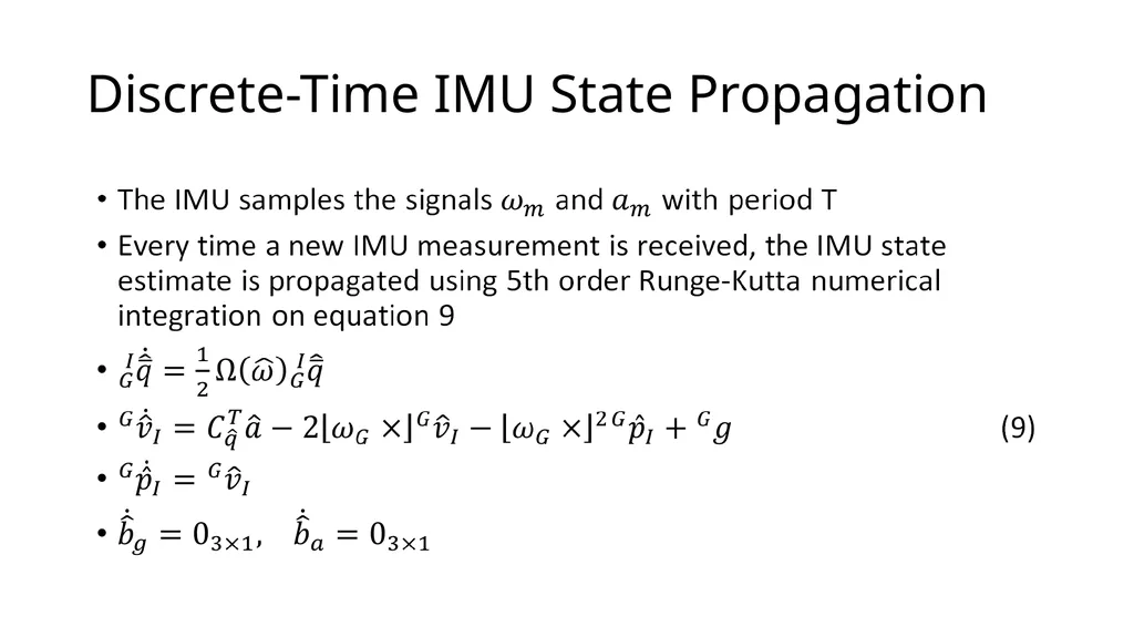
Discrete-Time IMU State Propagation<br>
28
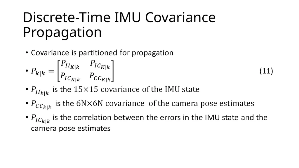
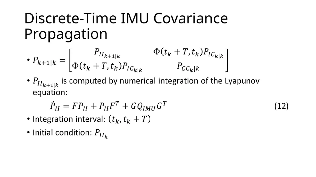
Discrete-Time IMU Covariance Propagation<br>
29
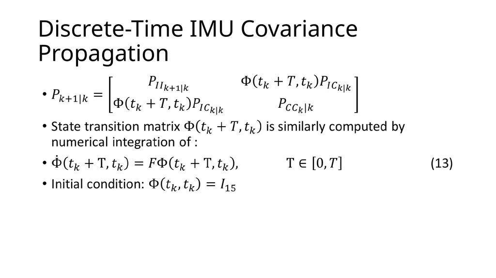
Discrete-Time IMU Covariance Propagation<br>
30
Discrete-Time IMU Covariance Propagation<br>
31
State Augmentation<br>
32
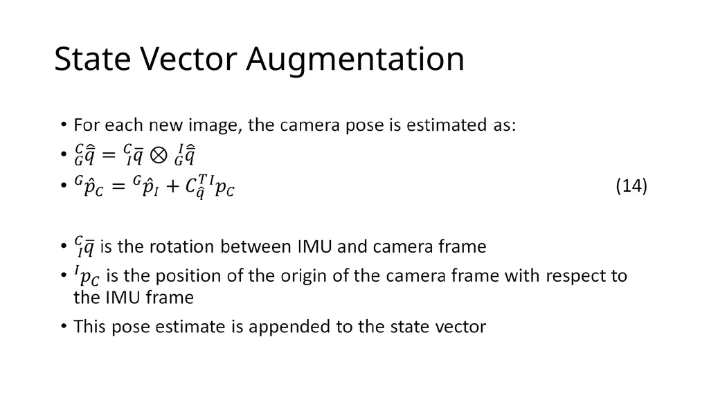
State Vector Augmentation<br>
33
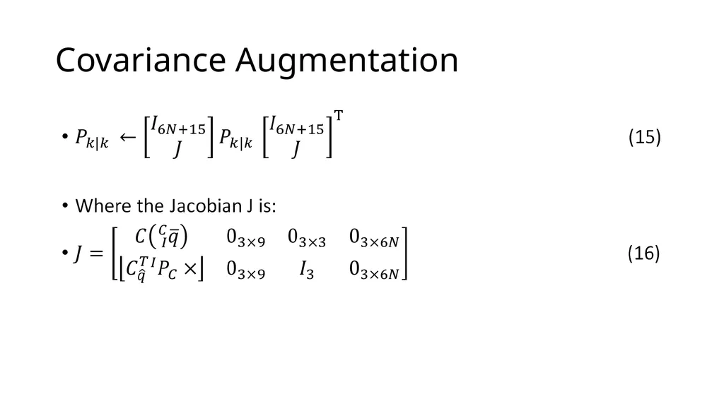
Covariance Augmentation<br>
35
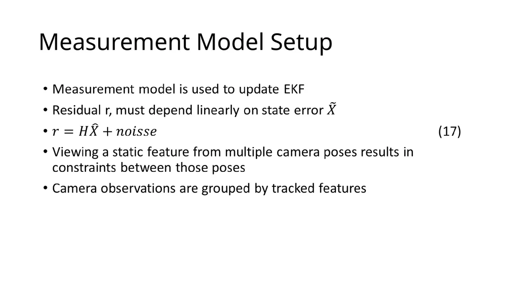
Measurement Model Setup<br>
36
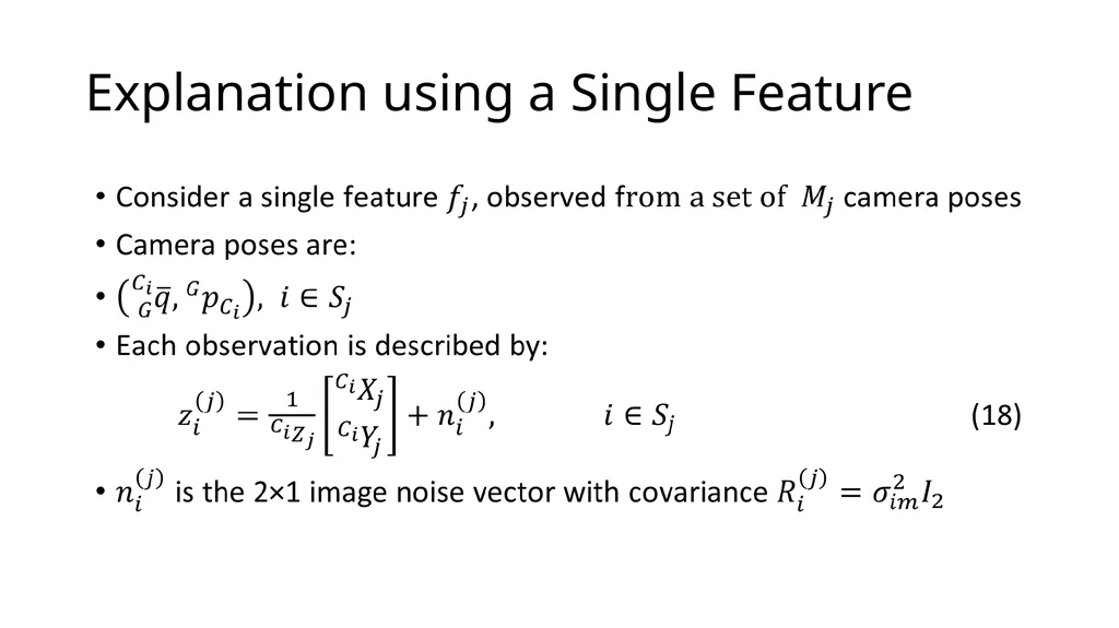
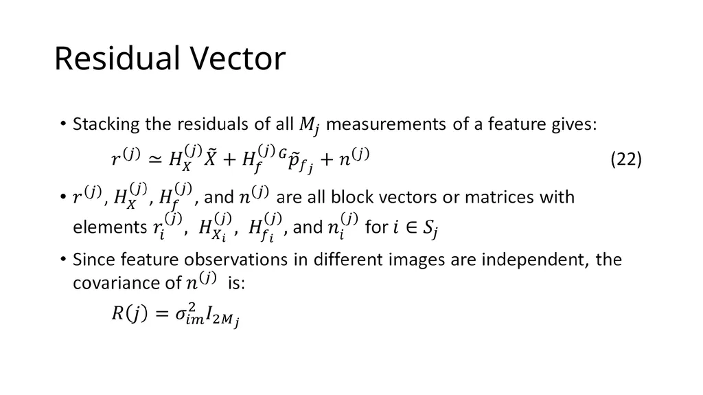
Explanation using a Single Feature<br>
37
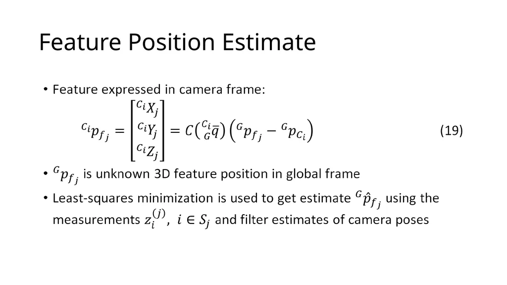
Feature Position Estimate<br>
38
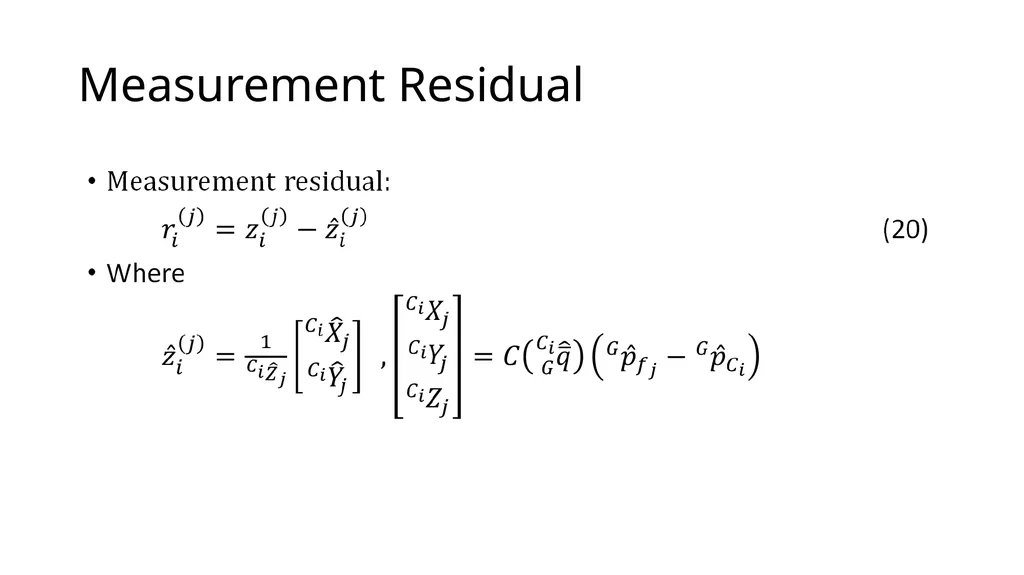
Measurement Residual<br>
39
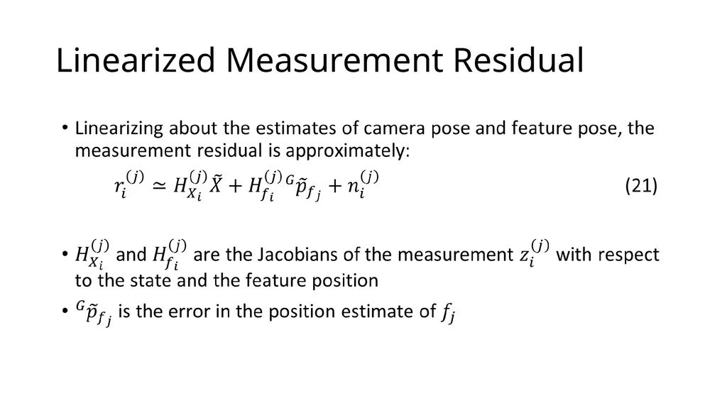
Linearized Measurement Residual<br>
41
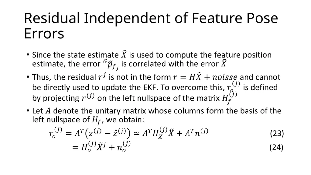
Residual Independent of Feature Pose Errors<br>
43
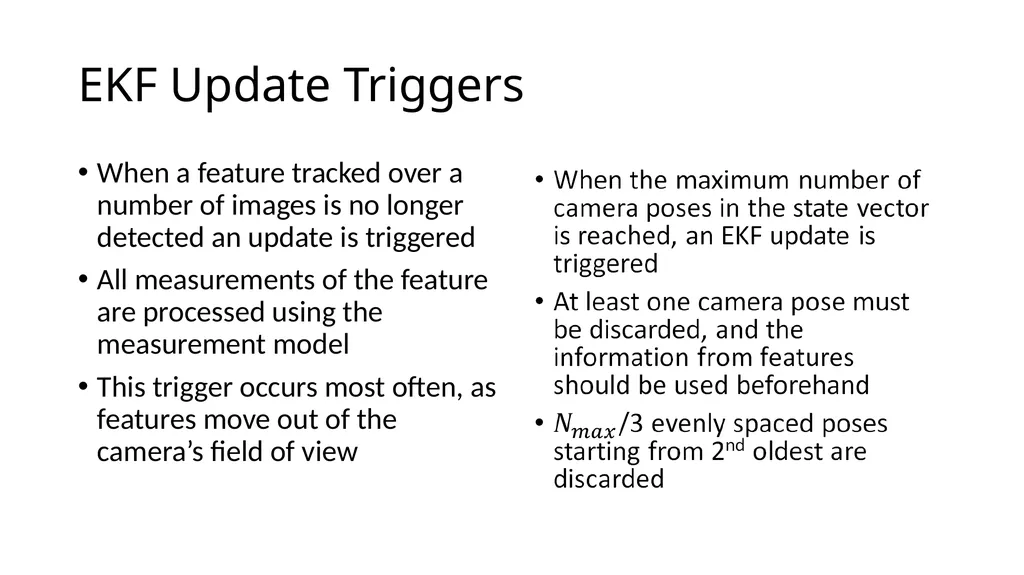
EKF Update Triggers When a feature tracked over a number of images is no longer detected an update is triggered
All measurements of the feature are processed using the measurement model
This trigger occurs most often, as features move out of the camera’s field of view<br>
45
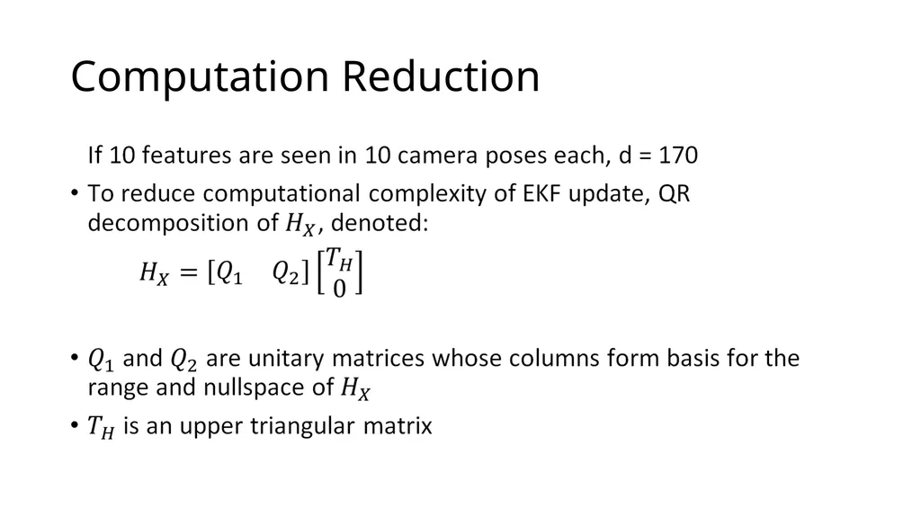
Computation Reduction<br>
46
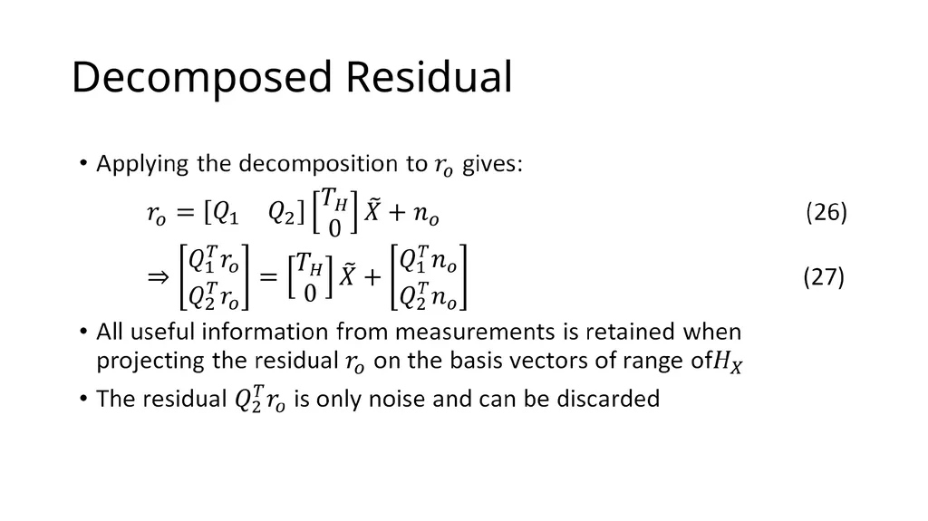
Decomposed Residual<br>
47
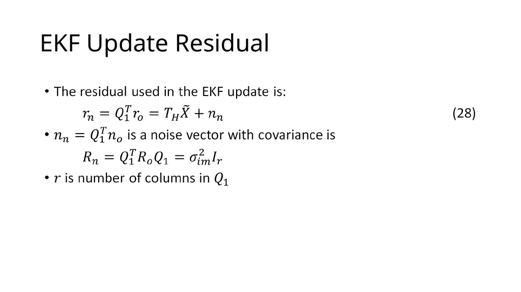
EKF Update Residual<br>
50
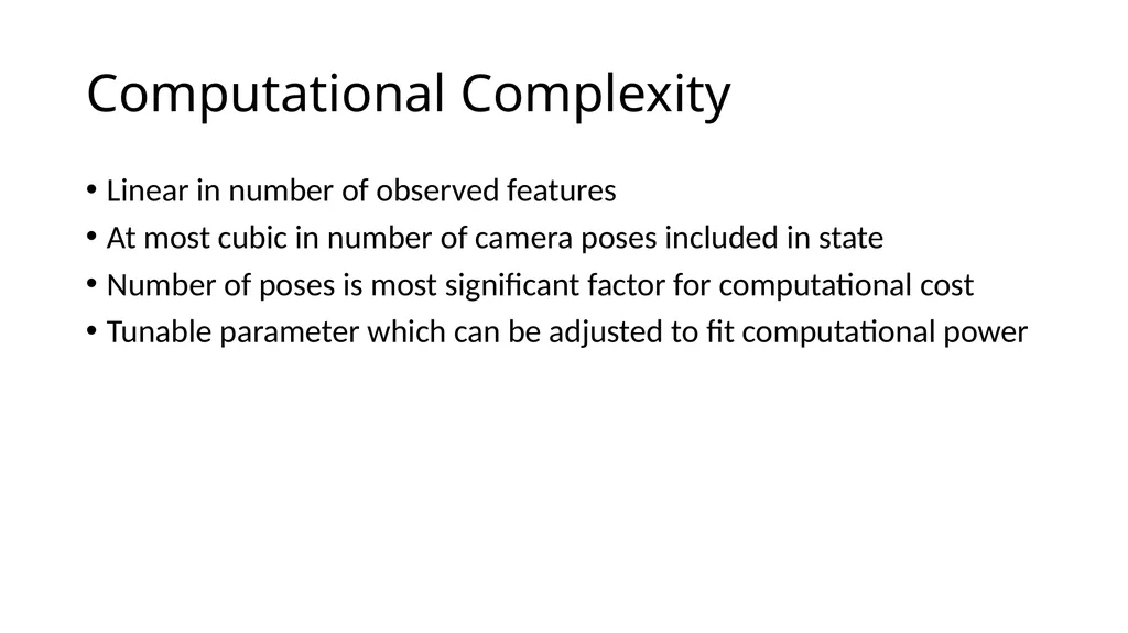
Computational Complexity Linear in number of observed features
At most cubic in number of camera poses included in state
Number of poses is most significant factor for computational cost
Tunable parameter which can be adjusted to fit computational power<br>
51
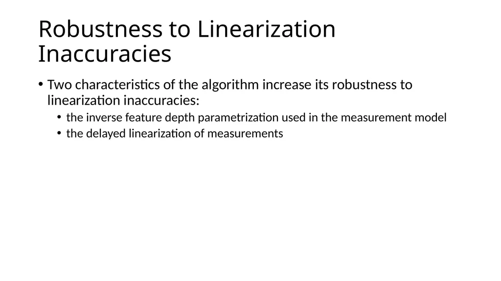
Robustness to Linearization Inaccuracies Two characteristics of the algorithm increase its robustness to linearization inaccuracies:
the inverse feature depth parametrization used in the measurement model
the delayed linearization of measurements<br>
52
Optimal for Many Features Two kinds of features:
Opportunistic Features – tracked over a small number of frames
Persistent Features – tracked over long period of time or when revisited
Opportunistic features are far more common
If all poses a feature is detected are in the state, the measurement model is optimal except for linearization inaccuracies
Therefore, the algorithm is able to optimally use localization information of opportunistic features<br>
53
Experimental Results<br>
56
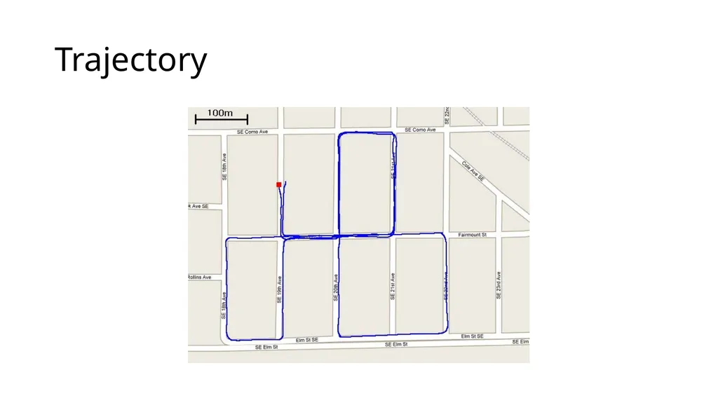
Results Dataset processed at 14Hz on a single core of a 2GHz processor
Since the start and end pose were known, the final position error was calculated to be approximately 10m
0.31% error over the 3.2km trajectory
No loop closure or nonholonomic constraints<br>