A Simple Subtraction Procedure for Calculation of
Description: A Simple Subtraction Procedure for Calculation of the Anomalous Magnetic Moment of the Electron in QED Sergey Volkov SINP MSU, Moscow Bogoliubov-Parasiuk theorem 1956 Removal of ultraviolet divergences by R-operation (defined by
Related Topics
Download Presentation
"A Simple Subtraction Procedure for Calculation of" is the property of its rightful owner. Permission is granted to download and print the materials on this website for personal, non-commercial use only, and to display it on your personal computer provided you do not modify the materials and that you retain all copyright notices contained in the materials. By downloading content from our website, you accept the terms of this agreement.
Presentation Transcript
slide1. A Simple Subtraction Procedure for Calculation of the Anomalous Magnetic Moment of the Electron in QED Sergey Volkov
SINP MSU, Moscow<br>
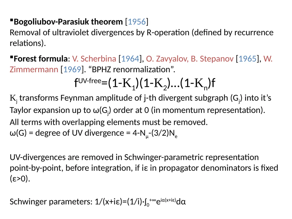
slide2. Bogoliubov-Parasiuk theorem [1956]
Removal of ultraviolet divergences by R-operation (defined by recurrence relations).
Forest formula: V. Scherbina [1964], O. Zavyalov, B. Stepanov [1965], W. Zimmermann [1969]. “BPHZ renormalization”.
fUV-free=(1-K1)(1-K2)…(1-Kn)f
Kj transforms Feynman amplitude of j-th divergent subgraph (Gj) into it’s Taylor expansion up to ω(Gj) order at 0 (in momentum representation).
All terms with overlapping elements must be removed.
ω(G) = degree of UV divergence = 4-Nμ-(3/2)Ne
UV-divergences are removed in Schwinger-parametric representation point-by-point, before integration, if iε in propagator denominators is fixed (ε>0).
Schwinger parameters: 1/(x+iε)=(1/i)·ʃ0+∞eiα(x+iε)dα
ε→0 => IR-divergences.<br>
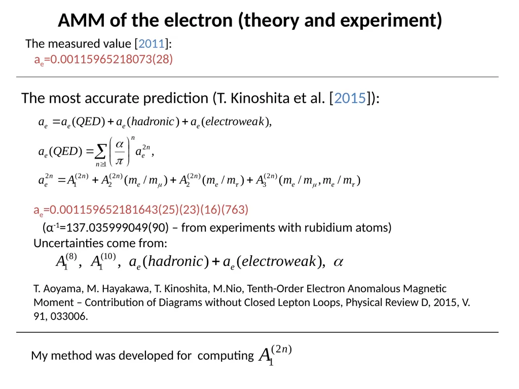
slide3. AMM of the electron (theory and experiment) The most accurate prediction (T. Kinoshita et al. [2015]): ae=0.001159652181643(25)(23)(16)(763)
(α-1=137.035999049(90) – from experiments with rubidium atoms)
Uncertainties come from:
T. Aoyama, M. Hayakawa, T. Kinoshita, M.Nio, Tenth-Order Electron Anomalous Magnetic Moment – Contribution of Diagrams without Closed Lepton Loops, Physical Review D, 2015, V. 91, 033006. The measured value [2011]:
ae=0.00115965218073(28) My method was developed for computing<br>
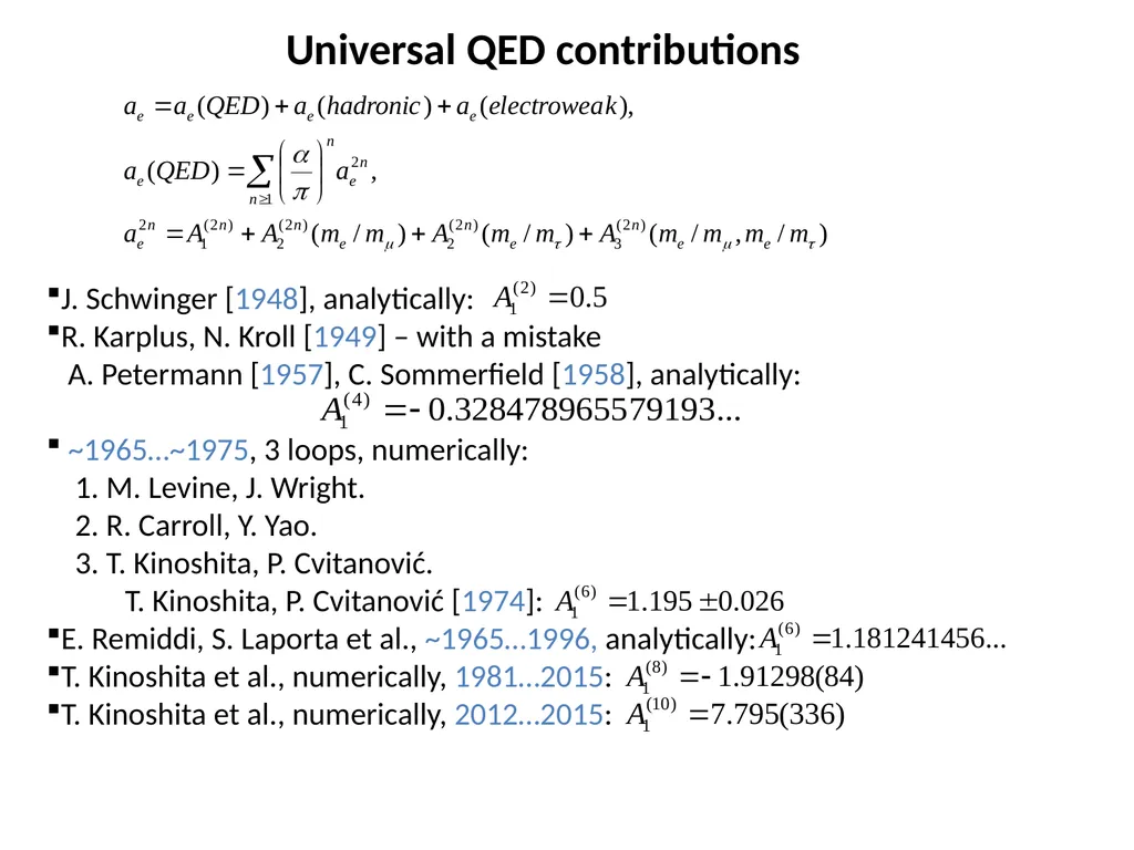
slide4. Universal QED contributions J. Schwinger [1948], analytically:
R. Karplus, N. Kroll [1949] – with a mistake
A. Petermann [1957], C. Sommerfield [1958], analytically:
~1965…~1975, 3 loops, numerically:
1. M. Levine, J. Wright.
2. R. Carroll, Y. Yao.
3. T. Kinoshita, P. Cvitanović.
T. Kinoshita, P. Cvitanović [1974]:
E. Remiddi, S. Laporta et al., ~1965…1996, analytically:
T. Kinoshita et al., numerically, 1981…2015:
T. Kinoshita et al., numerically, 2012…2015:<br>
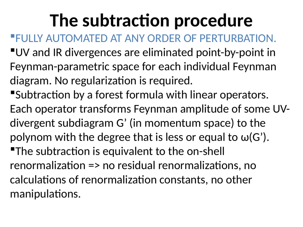
slide5. The subtraction procedure
FULLY AUTOMATED AT ANY ORDER OF PERTURBATION.
UV and IR divergences are eliminated point-by-point in Feynman-parametric space for each individual Feynman diagram. No regularization is required.
Subtraction by a forest formula with linear operators. Each operator transforms Feynman amplitude of some UV-divergent subdiagram G’ (in momentum space) to the polynom with the degree that is less or equal to ω(G’).
The subtraction is equivalent to the on-shell renormalization => no residual renormalizations, no calculations of renormalization constants, no other manipulations.<br>
slide6. Anomalous magnetic moment: definition p-q/2 p+q/2 q (renormalized)<br>
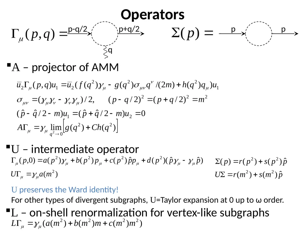
slide7. Operators p-q/2 p+q/2 q p p U – intermediate operator U preserves the Ward identity!
For other types of divergent subgraphs, U=Taylor expansion at 0 up to ω order.
L – on-shell renormalization for vertex-like subgraphs A – projector of AMM<br>
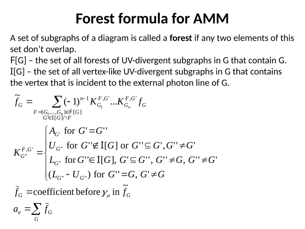
slide8. Forest formula for AMM
A set of subgraphs of a diagram is called a forest if any two elements of this set don’t overlap.
F[G] – the set of all forests of UV-divergent subgraphs in G that contain G.
I[G] – the set of all vertex-like UV-divergent subgraphs in G that contains the vertex that is incident to the external photon line of G.<br>
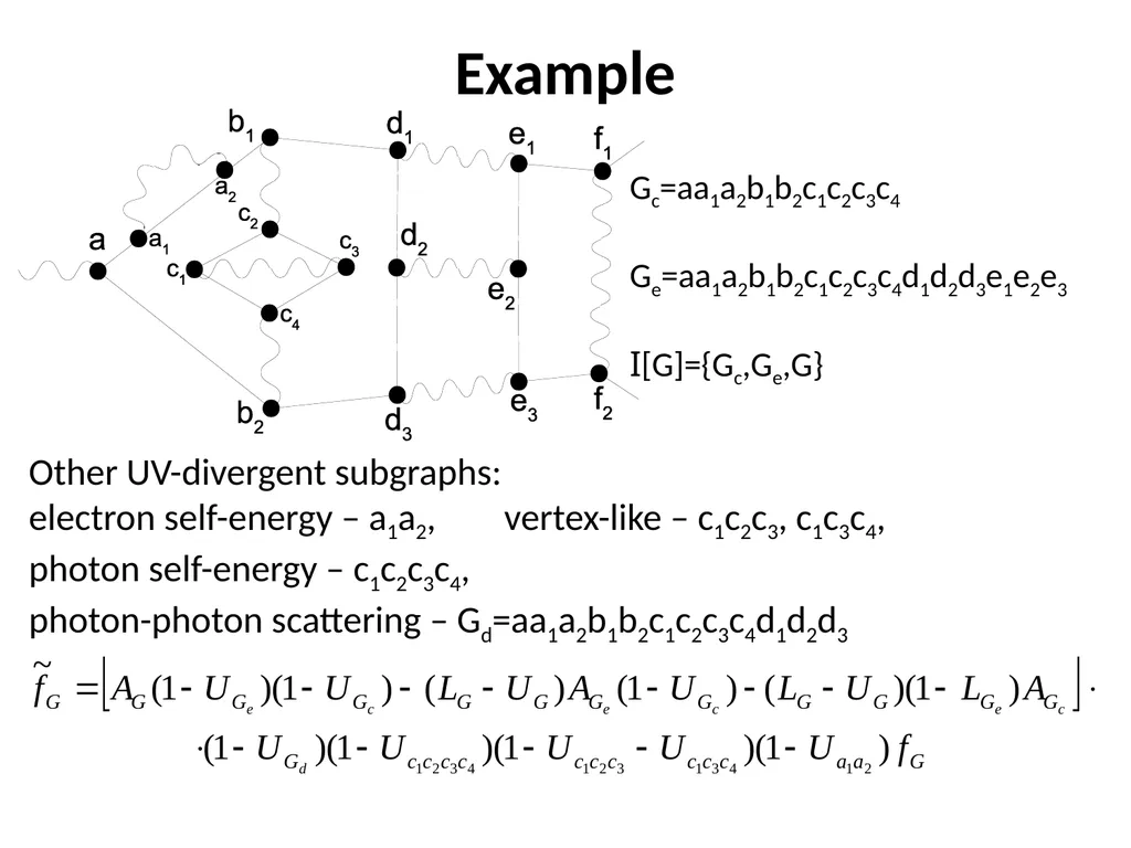
slide9. Example Gc=aa1a2b1b2c1c2c3c4
Ge=aa1a2b1b2c1c2c3c4d1d2d3e1e2e3
I[G]={Gc,Ge,G} Other UV-divergent subgraphs:
electron self-energy – a1a2, vertex-like – c1c2c3, c1c3c4,
photon self-energy – c1c2c3c4,
photon-photon scattering – Gd=aa1a2b1b2c1c2c3c4d1d2d3<br>
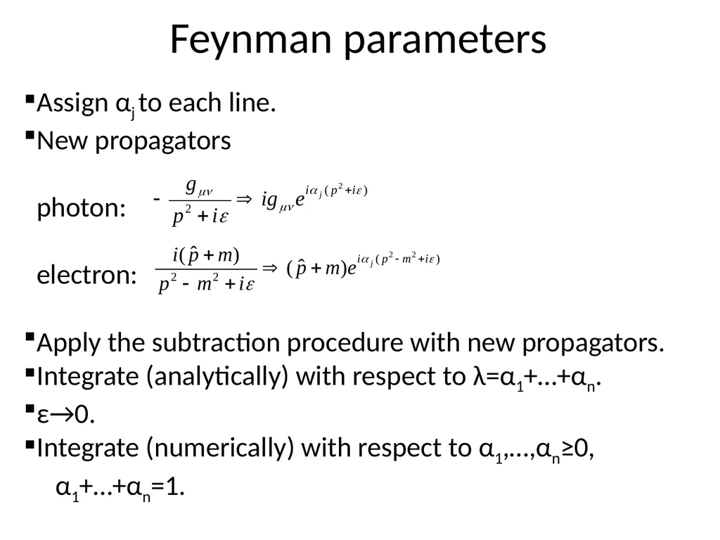
slide10. Feynman parameters Assign αj to each line.
New propagators
photon:
electron:
Apply the subtraction procedure with new propagators.
Integrate (analytically) with respect to λ=α1+…+αn.
ε→0.
Integrate (numerically) with respect to α1,…,αn≥0,
α1+…+αn=1.<br>
slide11. Realization
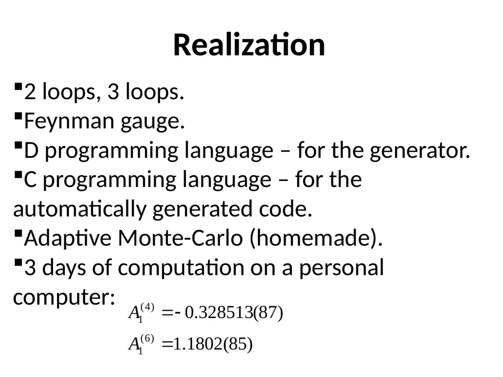
2 loops, 3 loops.
Feynman gauge.
D programming language – for the generator.
C programming language – for the automatically generated code.
Adaptive Monte-Carlo (homemade).
3 days of computation on a personal computer:<br>
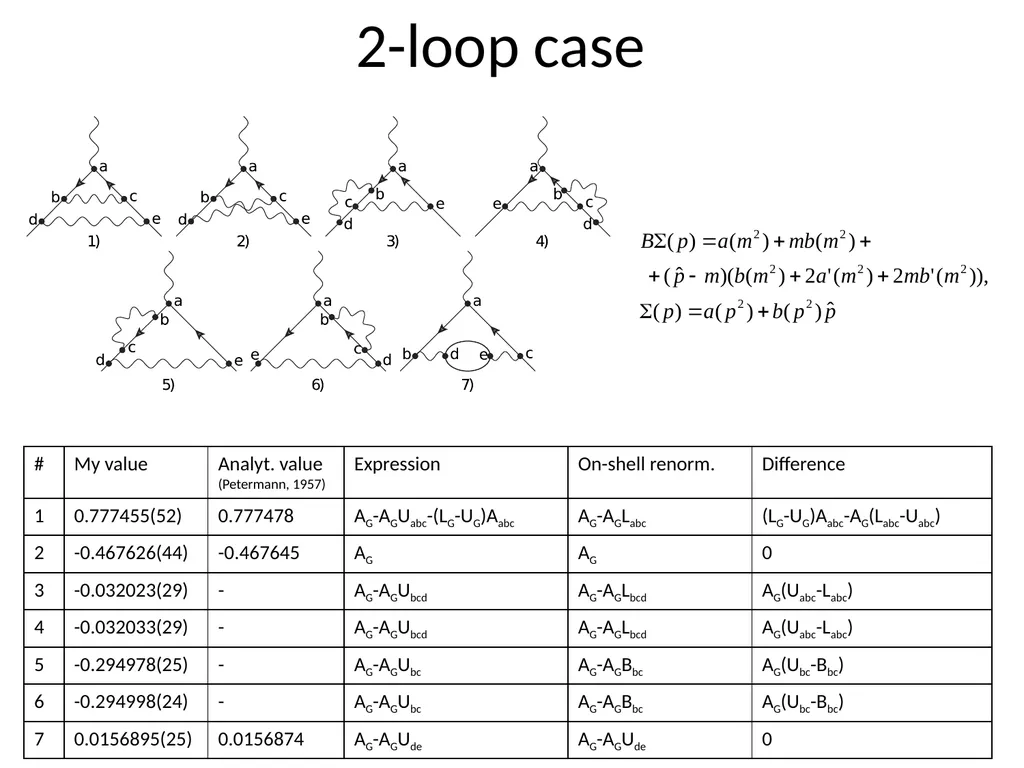
slide12. 2-loop case<br>
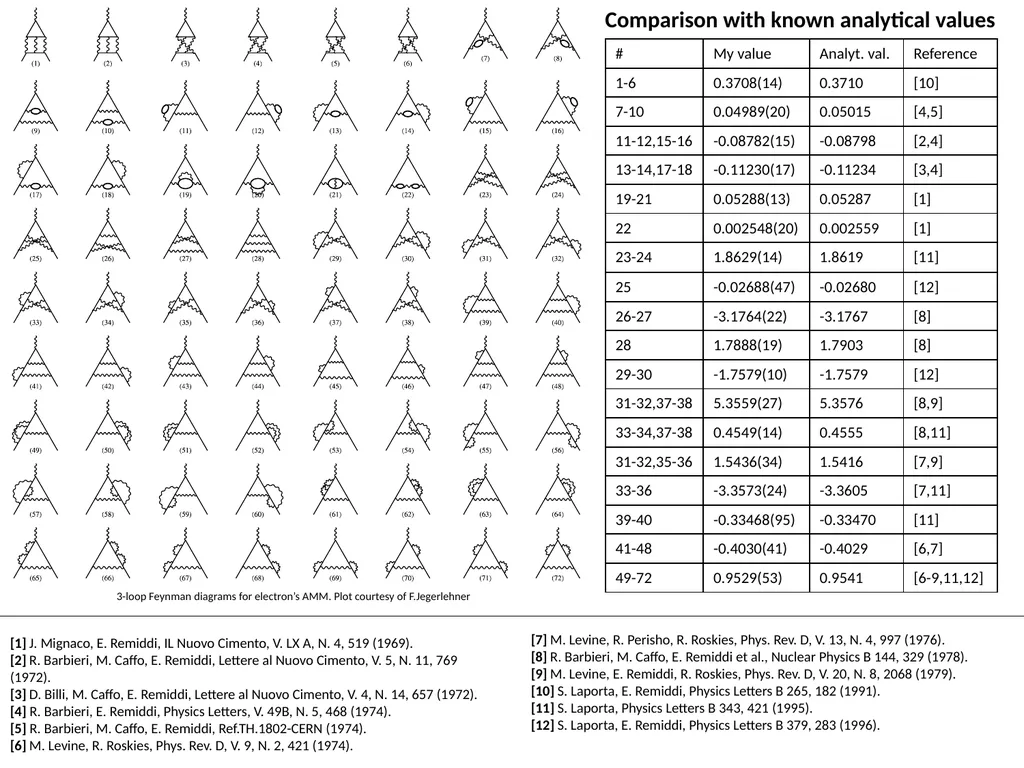
slide13. 3-loop Feynman diagrams for electron’s AMM. Plot courtesy of F.Jegerlehner [1] J. Mignaco, E. Remiddi, IL Nuovo Cimento, V. LX A, N. 4, 519 (1969).
[2] R. Barbieri, M. Caffo, E. Remiddi, Lettere al Nuovo Cimento, V. 5, N. 11, 769 (1972).
[3] D. Billi, M. Caffo, E. Remiddi, Lettere al Nuovo Cimento, V. 4, N. 14, 657 (1972).
[4] R. Barbieri, E. Remiddi, Physics Letters, V. 49B, N. 5, 468 (1974).
[5] R. Barbieri, M. Caffo, E. Remiddi, Ref.TH.1802-CERN (1974).
[6] M. Levine, R. Roskies, Phys. Rev. D, V. 9, N. 2, 421 (1974). [7] M. Levine, R. Perisho, R. Roskies, Phys. Rev. D, V. 13, N. 4, 997 (1976).
[8] R. Barbieri, M. Caffo, E. Remiddi et al., Nuclear Physics B 144, 329 (1978).
[9] M. Levine, E. Remiddi, R. Roskies, Phys. Rev. D, V. 20, N. 8, 2068 (1979).
[10] S. Laporta, E. Remiddi, Physics Letters B 265, 182 (1991).
[11] S. Laporta, Physics Letters B 343, 421 (1995).
[12] S. Laporta, E. Remiddi, Physics Letters B 379, 283 (1996). Comparison with known analytical values<br>
slide14. Thank you
for your attention! volkoff_sergey@mail.ru http://arxiv.org/abs/1507.06435<br>

SINP MSU, Moscow<br>
slide2. Bogoliubov-Parasiuk theorem [1956]
Removal of ultraviolet divergences by R-operation (defined by recurrence relations).
Forest formula: V. Scherbina [1964], O. Zavyalov, B. Stepanov [1965], W. Zimmermann [1969]. “BPHZ renormalization”.
fUV-free=(1-K1)(1-K2)…(1-Kn)f
Kj transforms Feynman amplitude of j-th divergent subgraph (Gj) into it’s Taylor expansion up to ω(Gj) order at 0 (in momentum representation).
All terms with overlapping elements must be removed.
ω(G) = degree of UV divergence = 4-Nμ-(3/2)Ne
UV-divergences are removed in Schwinger-parametric representation point-by-point, before integration, if iε in propagator denominators is fixed (ε>0).
Schwinger parameters: 1/(x+iε)=(1/i)·ʃ0+∞eiα(x+iε)dα
ε→0 => IR-divergences.<br>
slide3. AMM of the electron (theory and experiment) The most accurate prediction (T. Kinoshita et al. [2015]): ae=0.001159652181643(25)(23)(16)(763)
(α-1=137.035999049(90) – from experiments with rubidium atoms)
Uncertainties come from:
T. Aoyama, M. Hayakawa, T. Kinoshita, M.Nio, Tenth-Order Electron Anomalous Magnetic Moment – Contribution of Diagrams without Closed Lepton Loops, Physical Review D, 2015, V. 91, 033006. The measured value [2011]:
ae=0.00115965218073(28) My method was developed for computing<br>
slide4. Universal QED contributions J. Schwinger [1948], analytically:
R. Karplus, N. Kroll [1949] – with a mistake
A. Petermann [1957], C. Sommerfield [1958], analytically:
~1965…~1975, 3 loops, numerically:
1. M. Levine, J. Wright.
2. R. Carroll, Y. Yao.
3. T. Kinoshita, P. Cvitanović.
T. Kinoshita, P. Cvitanović [1974]:
E. Remiddi, S. Laporta et al., ~1965…1996, analytically:
T. Kinoshita et al., numerically, 1981…2015:
T. Kinoshita et al., numerically, 2012…2015:<br>
slide5. The subtraction procedure
FULLY AUTOMATED AT ANY ORDER OF PERTURBATION.
UV and IR divergences are eliminated point-by-point in Feynman-parametric space for each individual Feynman diagram. No regularization is required.
Subtraction by a forest formula with linear operators. Each operator transforms Feynman amplitude of some UV-divergent subdiagram G’ (in momentum space) to the polynom with the degree that is less or equal to ω(G’).
The subtraction is equivalent to the on-shell renormalization => no residual renormalizations, no calculations of renormalization constants, no other manipulations.<br>
slide6. Anomalous magnetic moment: definition p-q/2 p+q/2 q (renormalized)<br>
slide7. Operators p-q/2 p+q/2 q p p U – intermediate operator U preserves the Ward identity!
For other types of divergent subgraphs, U=Taylor expansion at 0 up to ω order.
L – on-shell renormalization for vertex-like subgraphs A – projector of AMM<br>
slide8. Forest formula for AMM
A set of subgraphs of a diagram is called a forest if any two elements of this set don’t overlap.
F[G] – the set of all forests of UV-divergent subgraphs in G that contain G.
I[G] – the set of all vertex-like UV-divergent subgraphs in G that contains the vertex that is incident to the external photon line of G.<br>
slide9. Example Gc=aa1a2b1b2c1c2c3c4
Ge=aa1a2b1b2c1c2c3c4d1d2d3e1e2e3
I[G]={Gc,Ge,G} Other UV-divergent subgraphs:
electron self-energy – a1a2, vertex-like – c1c2c3, c1c3c4,
photon self-energy – c1c2c3c4,
photon-photon scattering – Gd=aa1a2b1b2c1c2c3c4d1d2d3<br>
slide10. Feynman parameters Assign αj to each line.
New propagators
photon:
electron:
Apply the subtraction procedure with new propagators.
Integrate (analytically) with respect to λ=α1+…+αn.
ε→0.
Integrate (numerically) with respect to α1,…,αn≥0,
α1+…+αn=1.<br>
slide11. Realization
2 loops, 3 loops.
Feynman gauge.
D programming language – for the generator.
C programming language – for the automatically generated code.
Adaptive Monte-Carlo (homemade).
3 days of computation on a personal computer:<br>
slide12. 2-loop case<br>
slide13. 3-loop Feynman diagrams for electron’s AMM. Plot courtesy of F.Jegerlehner [1] J. Mignaco, E. Remiddi, IL Nuovo Cimento, V. LX A, N. 4, 519 (1969).
[2] R. Barbieri, M. Caffo, E. Remiddi, Lettere al Nuovo Cimento, V. 5, N. 11, 769 (1972).
[3] D. Billi, M. Caffo, E. Remiddi, Lettere al Nuovo Cimento, V. 4, N. 14, 657 (1972).
[4] R. Barbieri, E. Remiddi, Physics Letters, V. 49B, N. 5, 468 (1974).
[5] R. Barbieri, M. Caffo, E. Remiddi, Ref.TH.1802-CERN (1974).
[6] M. Levine, R. Roskies, Phys. Rev. D, V. 9, N. 2, 421 (1974). [7] M. Levine, R. Perisho, R. Roskies, Phys. Rev. D, V. 13, N. 4, 997 (1976).
[8] R. Barbieri, M. Caffo, E. Remiddi et al., Nuclear Physics B 144, 329 (1978).
[9] M. Levine, E. Remiddi, R. Roskies, Phys. Rev. D, V. 20, N. 8, 2068 (1979).
[10] S. Laporta, E. Remiddi, Physics Letters B 265, 182 (1991).
[11] S. Laporta, Physics Letters B 343, 421 (1995).
[12] S. Laporta, E. Remiddi, Physics Letters B 379, 283 (1996). Comparison with known analytical values<br>
slide14. Thank you
for your attention! volkoff_sergey@mail.ru http://arxiv.org/abs/1507.06435<br>