Aaron Tan 5 9 November 2018 12. Graphs and Trees 2 Summary 1 2 12. Graphs and Trees 2 Summary 3 10.5 Trees Summary 4 10.5 Trees Summary 5 10.6 Rooted Trees Summary 6 10.6 Rooted Trees Summary 7 10.6 Rooted Trees Summary 8 10.6 Rooted
"Aaron Tan 5 – 9 November 2018 12. Graphs and" is the property of its rightful owner. Permission is granted to
download and print the materials on this website for personal, non-commercial use only, and to display it
on your personal computer provided you do not modify the materials and that you retain all copyright
notices contained in the materials. By downloading content from our website, you accept the terms of this
agreement.
Presentation Transcript
01
Aaron Tan
5 – 9 November 2018 12. Graphs and Trees 2 Summary 1<br>
02
2 12. Graphs and Trees 2 Summary<br>
03
3 10.5 Trees Summary<br>
04
4 10.5 Trees Summary<br>
05
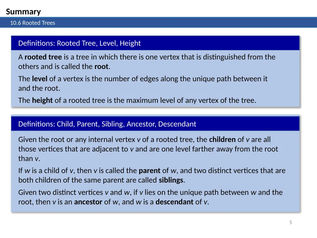
5 10.6 Rooted Trees Summary<br>
06
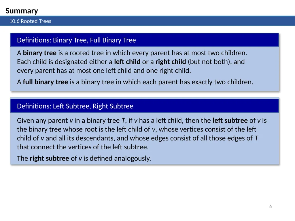
6 10.6 Rooted Trees Summary<br>
07
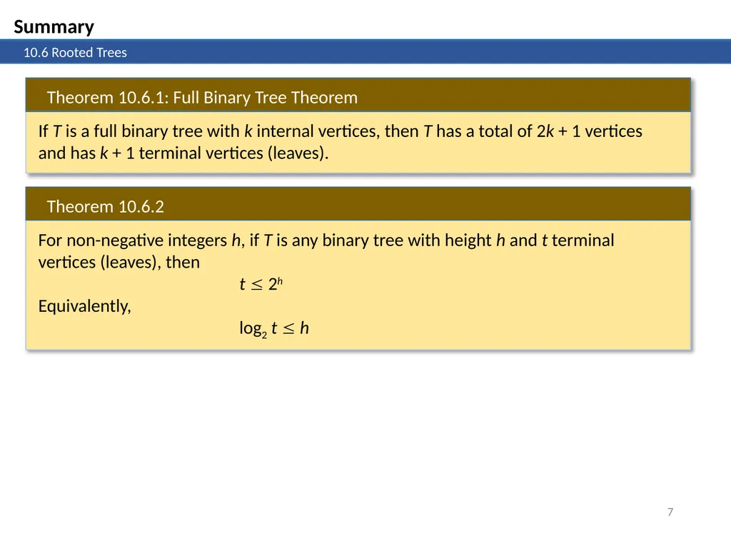
7 10.6 Rooted Trees Summary<br>
08
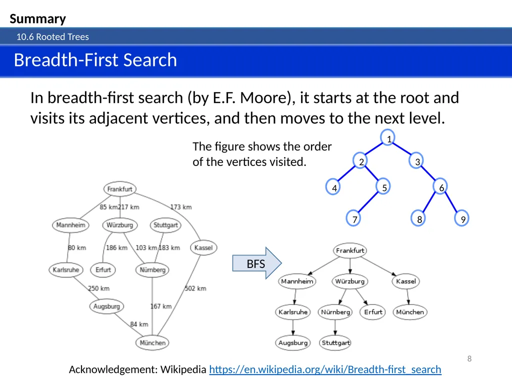
8 10.6 Rooted Trees Summary Breadth-First Search In breadth-first search (by E.F. Moore), it starts at the root and visits its adjacent vertices, and then moves to the next level. The figure shows the order of the vertices visited. BFS Acknowledgement: Wikipedia https://en.wikipedia.org/wiki/Breadth-first_search<br>
09
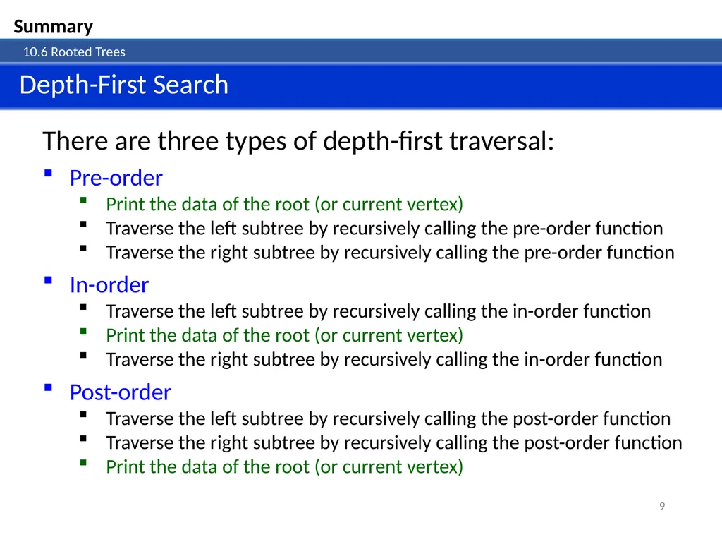
9 10.6 Rooted Trees Summary Depth-First Search There are three types of depth-first traversal:
Pre-order
Print the data of the root (or current vertex)
Traverse the left subtree by recursively calling the pre-order function
Traverse the right subtree by recursively calling the pre-order function
In-order
Traverse the left subtree by recursively calling the in-order function
Print the data of the root (or current vertex)
Traverse the right subtree by recursively calling the in-order function
Post-order
Traverse the left subtree by recursively calling the post-order function
Traverse the right subtree by recursively calling the post-order function
Print the data of the root (or current vertex)<br>
10
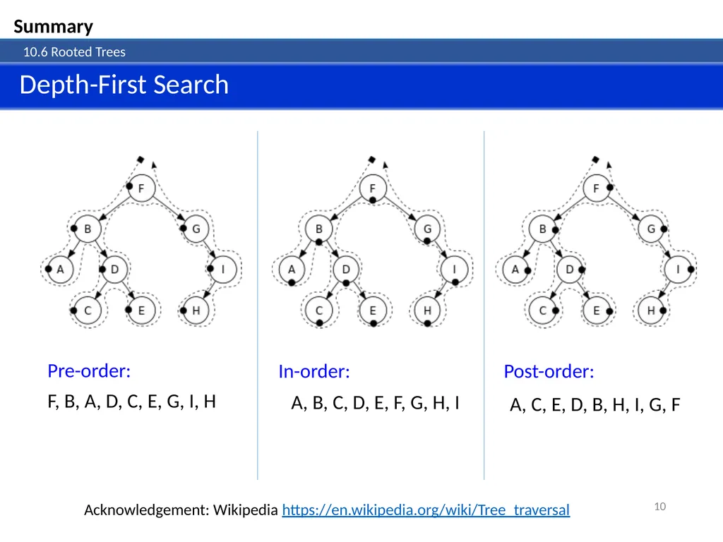
10 10.6 Rooted Trees Summary Depth-First Search Pre-order:
F, B, A, D, C, E, G, I, H In-order: Post-order: A, B, C, D, E, F, G, H, I A, C, E, D, B, H, I, G, F Acknowledgement: Wikipedia https://en.wikipedia.org/wiki/Tree_traversal<br>
11
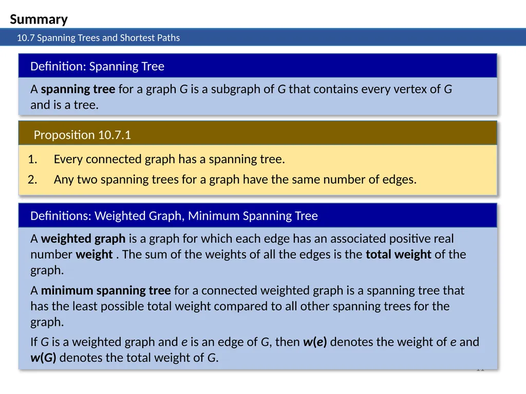
11 10.7 Spanning Trees and Shortest Paths Summary<br>
12
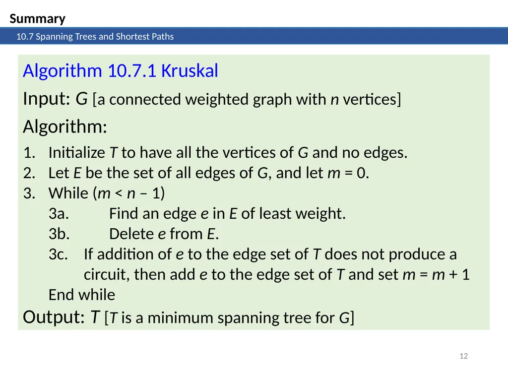
12 10.7 Spanning Trees and Shortest Paths Summary Algorithm 10.7.1 Kruskal
Input: G [a connected weighted graph with n vertices]
Algorithm:
Initialize T to have all the vertices of G and no edges.
Let E be the set of all edges of G, and let m = 0.
While (m < n – 1)
3a. Find an edge e in E of least weight.
3b. Delete e from E.
3c. If addition of e to the edge set of T does not produce a circuit, then add e to the edge set of T and set m = m + 1
End while
Output: T [T is a minimum spanning tree for G]<br>
13
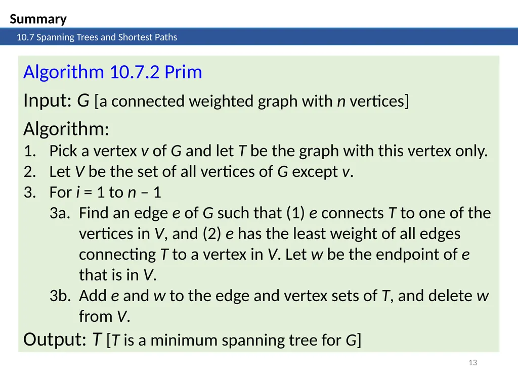
13 10.7 Spanning Trees and Shortest Paths Summary Algorithm 10.7.2 Prim
Input: G [a connected weighted graph with n vertices]
Algorithm:
Pick a vertex v of G and let T be the graph with this vertex only.
Let V be the set of all vertices of G except v.
For i = 1 to n – 1
3a. Find an edge e of G such that (1) e connects T to one of the vertices in V, and (2) e has the least weight of all edges connecting T to a vertex in V. Let w be the endpoint of e that is in V.
3b. Add e and w to the edge and vertex sets of T, and delete w from V.
Output: T [T is a minimum spanning tree for G]<br>
14
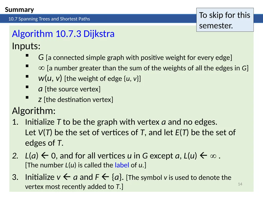
Algorithm 10.7.3 Dijkstra
Inputs:
G [a connected simple graph with positive weight for every edge]
[a number greater than the sum of the weights of all the edges in G]
w(u, v) [the weight of edge {u, v}]
a [the source vertex]
z [the destination vertex]
Algorithm:
Initialize T to be the graph with vertex a and no edges. Let V(T) be the set of vertices of T, and let E(T) be the set of edges of T.
L(a) 0, and for all vertices u in G except a, L(u) . [The number L(u) is called the label of u.]
Initialize v a and F {a}. [The symbol v is used to denote the vertex most recently added to T.] 14 10.7 Spanning Trees and Shortest Paths Summary To skip for this semester.<br>
15
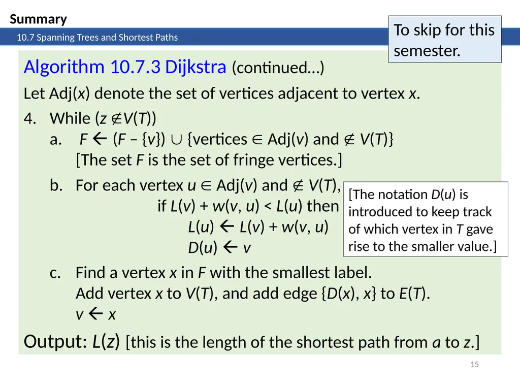
15 10.7 Spanning Trees and Shortest Paths Summary Algorithm 10.7.3 Dijkstra (continued…)
Let Adj(x) denote the set of vertices adjacent to vertex x.
While (z V(T))
F (F – {v}) {vertices Adj(v) and V(T)} [The set F is the set of fringe vertices.]
For each vertex u Adj(v) and V(T), if L(v) + w(v, u) < L(u) then L(u) L(v) + w(v, u) D(u) v
Find a vertex x in F with the smallest label. Add vertex x to V(T), and add edge {D(x), x} to E(T). v x
Output: L(z) [this is the length of the shortest path from a to z.] [The notation D(u) is introduced to keep track of which vertex in T gave rise to the smaller value.] To skip for this semester.<br>