
An Optimal Algorithm for Minimum-Link Rectilinear


Description: An Optimal Algorithm for Minimum-Link Rectilinear Paths in Triangulated Rectilinear Domains Joseph S.B. Mitchell, Stony Brook University Valentin Polishchuk, Linköping University Mikko Sysikaski, Google Zurich Haitao Wang, Utah State
Related Topics
Download Presentation
"An Optimal Algorithm for Minimum-Link Rectilinear" is the property of its rightful owner. Permission is granted to download and print the materials on this website for personal, non-commercial use only, and to display it on your personal computer provided you do not modify the materials and that you retain all copyright notices contained in the materials. By downloading content from our website, you accept the terms of this agreement.
Presentation Transcript
slide1. An Optimal Algorithm for Minimum-Link Rectilinear Paths in
Triangulated Rectilinear Domains Joseph S.B. Mitchell, Stony Brook University
Valentin Polishchuk, Linköping University
Mikko Sysikaski, Google Zurich
Haitao Wang, Utah State University
ICALP 2015<br>
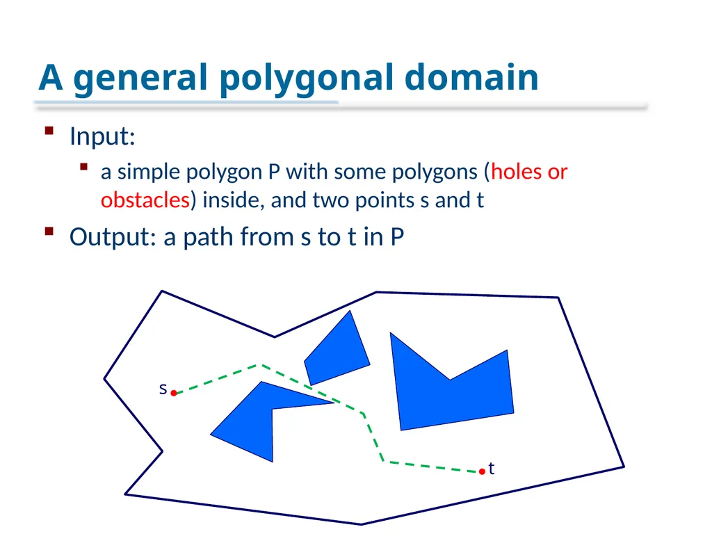
slide2. A general polygonal domain Input:
a simple polygon P with some polygons (holes or obstacles) inside, and two points s and t
Output: a path from s to t in P s t<br>
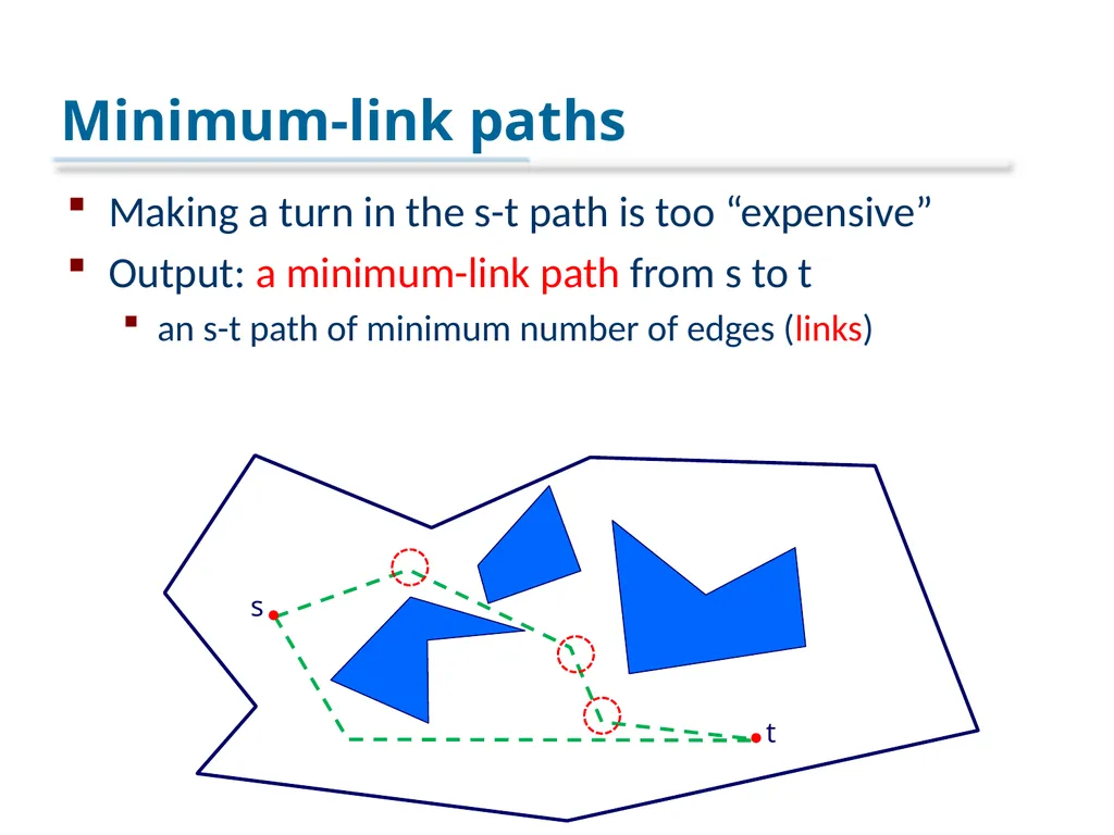
slide3. Minimum-link paths Making a turn in the s-t path is too “expensive”
Output: a minimum-link path from s to t
an s-t path of minimum number of edges (links) s t<br>
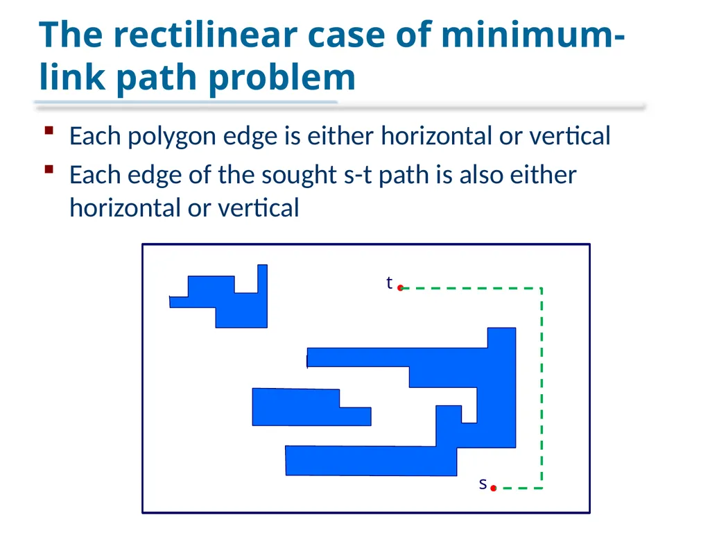
slide4. The rectilinear case of minimum-link path problem Each polygon edge is either horizontal or vertical
Each edge of the sought s-t path is also either horizontal or vertical s t<br>
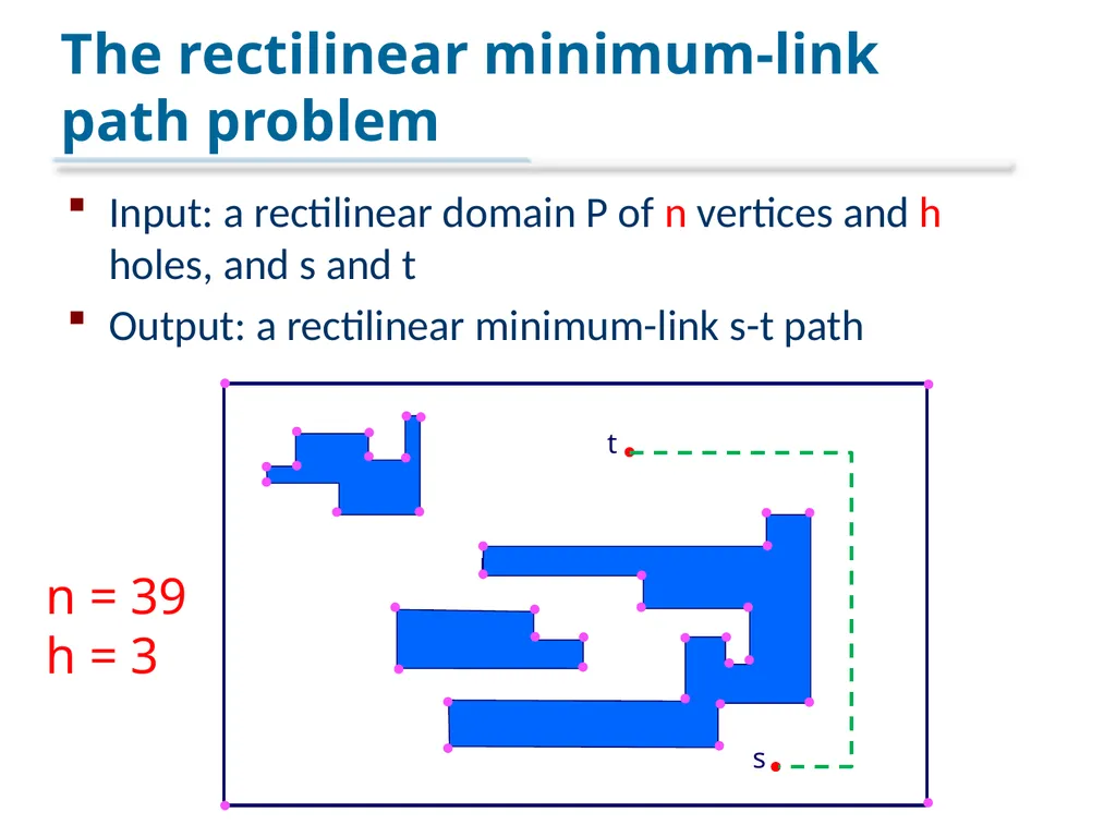
slide5. The rectilinear minimum-link path problem Input: a rectilinear domain P of n vertices and h holes, and s and t
Output: a rectilinear minimum-link s-t path s t n = 39
h = 3<br>
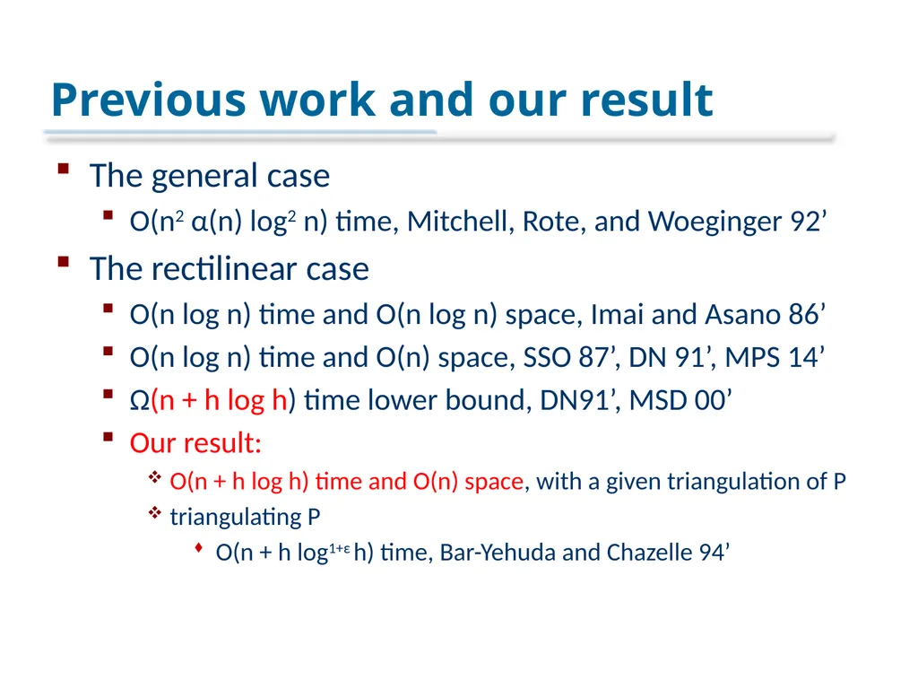
slide6. Previous work and our result The general case
O(n2 α(n) log2 n) time, Mitchell, Rote, and Woeginger 92’
The rectilinear case
O(n log n) time and O(n log n) space, Imai and Asano 86’
O(n log n) time and O(n) space, SSO 87’, DN 91’, MPS 14’
Ω(n + h log h) time lower bound, DN91’, MSD 00’
Our result:
O(n + h log h) time and O(n) space, with a given triangulation of P
triangulating P
O(n + h log1+ε h) time, Bar-Yehuda and Chazelle 94’<br>
slide7. Our result: answering single-source queries Build a data structure in O(n + h log h) time and O(n) space for s, to answer the queries:
given any query point t,
compute the link distance (the number of links of the rectilinear minimum-link s-t path) in O(log n) time
report the actual path in additional time linear in the link distance<br>
slide8. Outline The previous work: Das and Narasimhan, 91’
Our improvement based on their work<br>
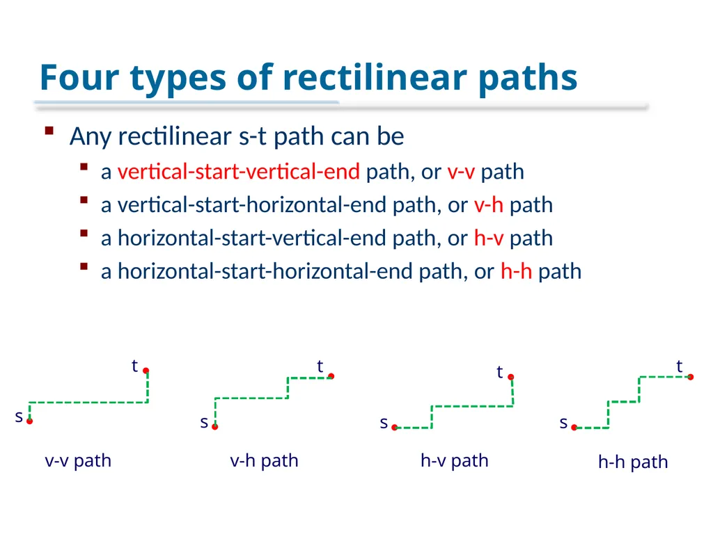
slide9. Four types of rectilinear paths Any rectilinear s-t path can be
a vertical-start-vertical-end path, or v-v path
a vertical-start-horizontal-end path, or v-h path
a horizontal-start-vertical-end path, or h-v path
a horizontal-start-horizontal-end path, or h-h path t s t s t s t s v-v path v-h path h-v path h-h path<br>
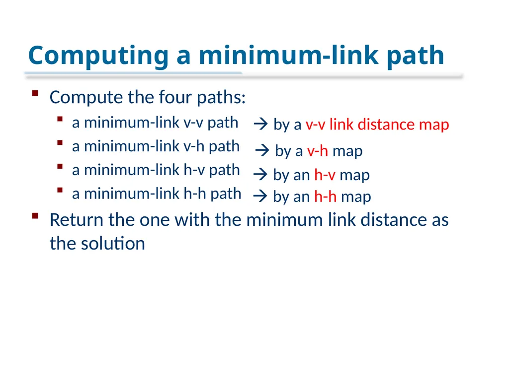
slide10. Computing a minimum-link path Compute the four paths:
a minimum-link v-v path
a minimum-link v-h path
a minimum-link h-v path
a minimum-link h-h path
Return the one with the minimum link distance as the solution by a v-v link distance map by a v-h map by an h-v map by an h-h map<br>
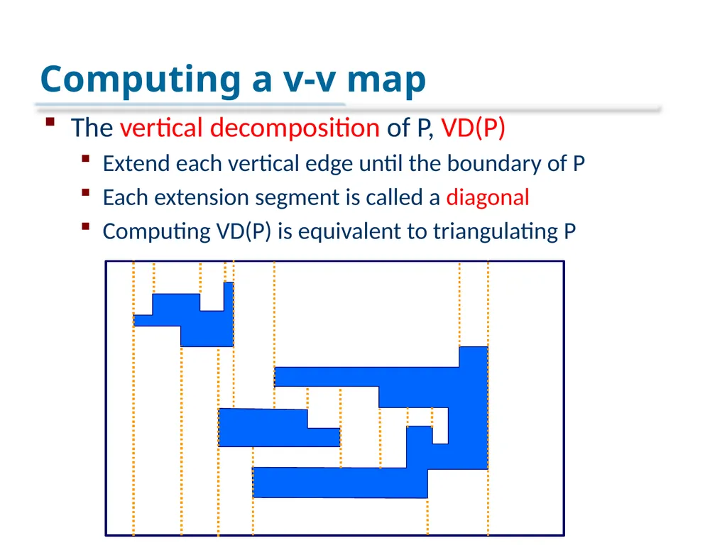
slide11. Computing a v-v map The vertical decomposition of P, VD(P)
Extend each vertical edge until the boundary of P
Each extension segment is called a diagonal
Computing VD(P) is equivalent to triangulating P<br>
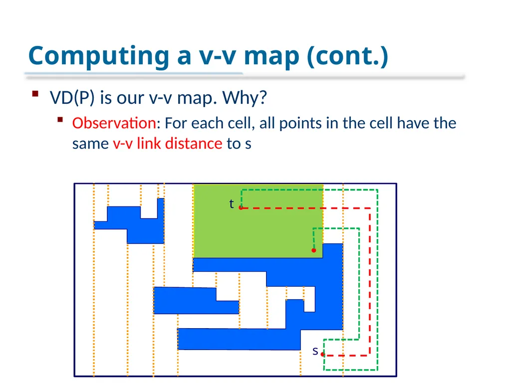
slide12. Computing a v-v map (cont.) VD(P) is our v-v map. Why?
Observation: For each cell, all points in the cell have the same v-v link distance to s s t<br>
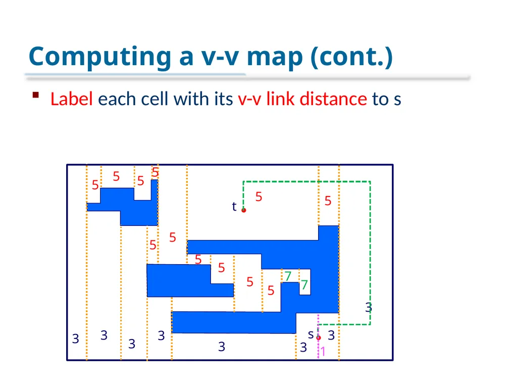
slide13. Computing a v-v map (cont.) Label each cell with its v-v link distance to s s 3 3 3 3 3 3 5 5 5 5 5 5 5 5 5 5 5 5 7 7 t 1 3 3<br>
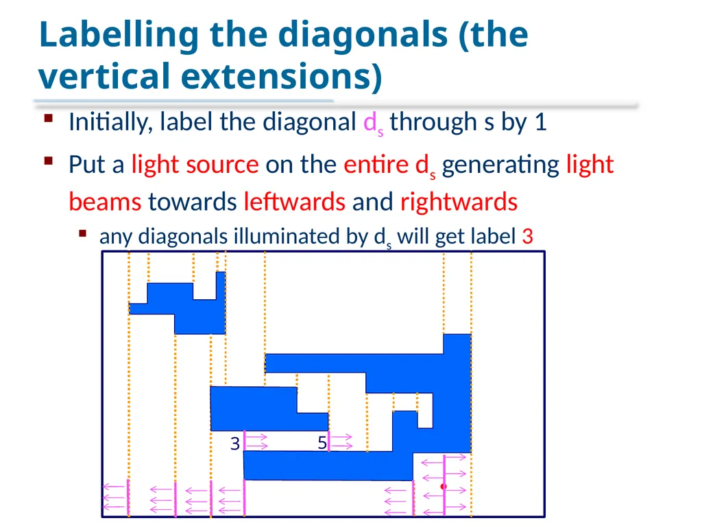
slide14. Labelling the diagonals (the vertical extensions) Initially, label the diagonal ds through s by 1
Put a light source on the entire ds generating light beams towards leftwards and rightwards
any diagonals illuminated by ds will get label 3 3 5<br>
slide15. The algorithm in the previous work In the i-th round, for i = 0, 1, 2, 3…..
Finds a set Vi of diagonals and label them 2i + 1
What is Vi ?
If we put light sources on all diagonals of Vi-1, then Vi consists of all new diagonals that can be illuminated
Two sweeping procedures: left-sweep and right-sweep
A heap is used to guide the sweeping such that the diagonals are processed by their x-coordinates
The sweeping is controlled in a global manner
O(n log n) time in total<br>
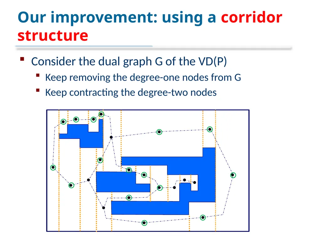
slide16. Our improvement: using a corridor structure Consider the dual graph G of the VD(P)
Keep removing the degree-one nodes from G
Keep contracting the degree-two nodes<br>
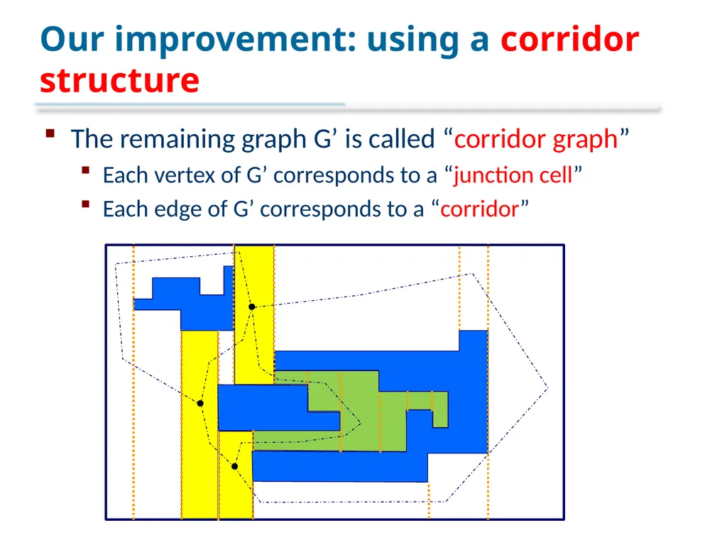
slide17. Our improvement: using a corridor structure The remaining graph G’ is called “corridor graph”
Each vertex of G’ corresponds to a “junction cell”
Each edge of G’ corresponds to a “corridor”<br>
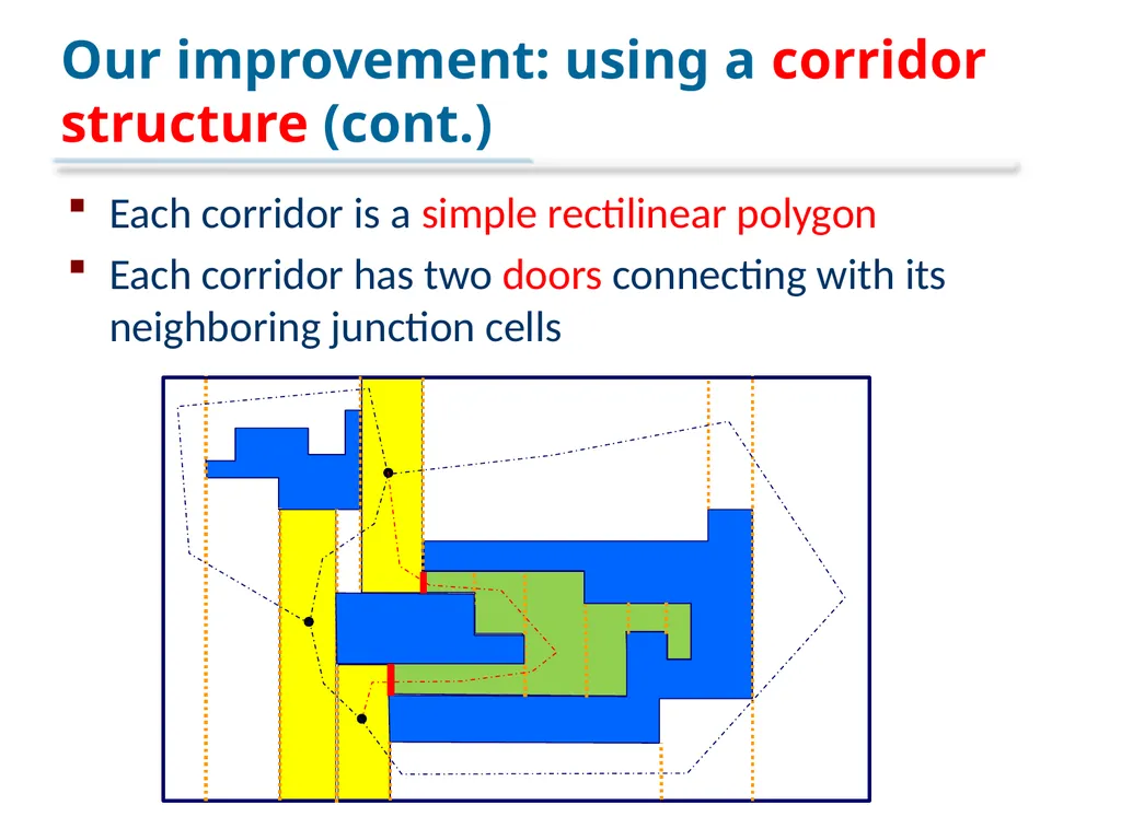
slide18. Our improvement: using a corridor structure (cont.) Each corridor is a simple rectilinear polygon
Each corridor has two doors connecting with its neighboring junction cells<br>
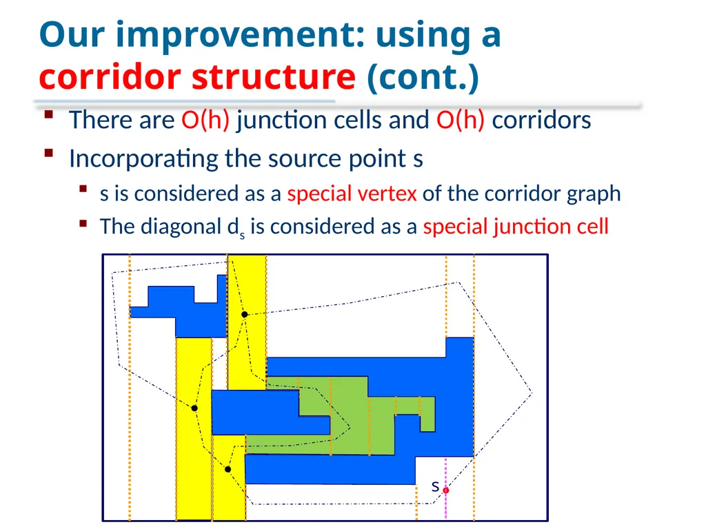
slide19. Our improvement: using a corridor structure (cont.) There are O(h) junction cells and O(h) corridors
Incorporating the source point s
s is considered as a special vertex of the corridor graph
The diagonal ds is considered as a special junction cell s<br>
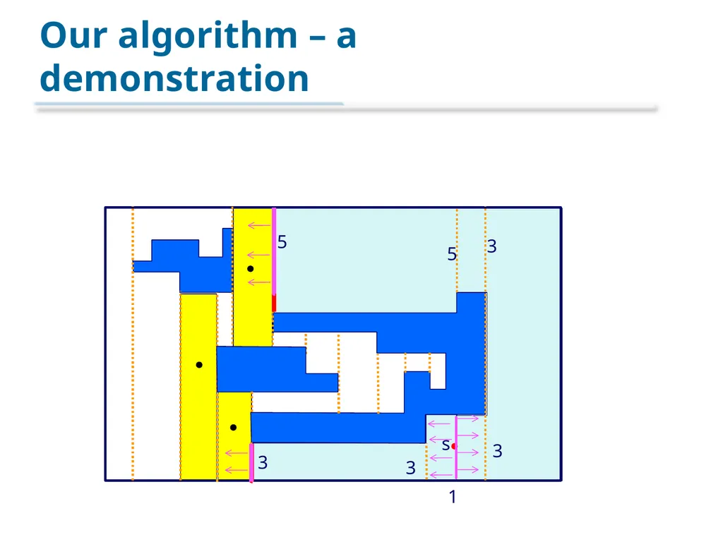
slide20. Our algorithm – an overview We use the same sweeping approach as before with the following differences
The sweeping in the junction cells is controlled in a global manner, the same as before
Once the sweeping enters into a corridor C through one of its doors, we sweep C in a local manner
What is the benefit?
The global sweeping is only on junction cells
There are only O(h) junction cells O(h log h) time
The local sweeping in each corridor can be processed in linear time since it is a simple polygon
The total size of all corridors is O(n) O(n) time<br>
slide21. Our algorithm – a demonstration s 1 5 5 3 3 3 3<br>
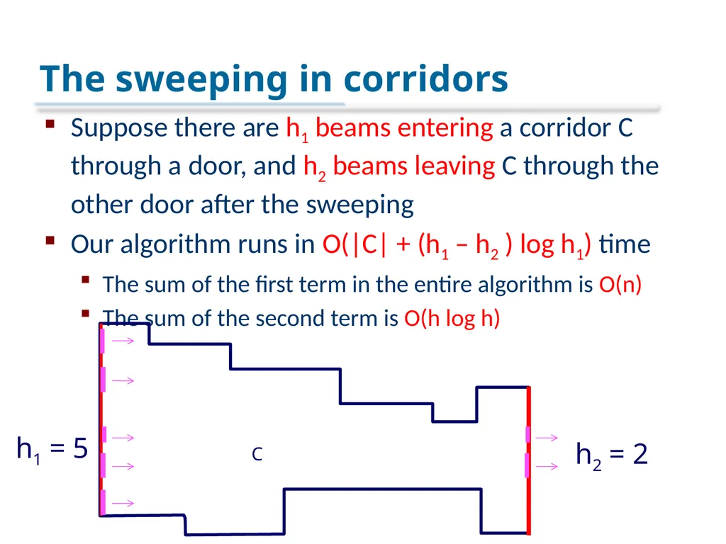
slide22. The sweeping in corridors Suppose there are h1 beams entering a corridor C through a door, and h2 beams leaving C through the other door after the sweeping
Our algorithm runs in O(|C| + (h1 – h2 ) log h1) time
The sum of the first term in the entire algorithm is O(n)
The sum of the second term is O(h log h) h1 = 5 h2 = 2 C<br>
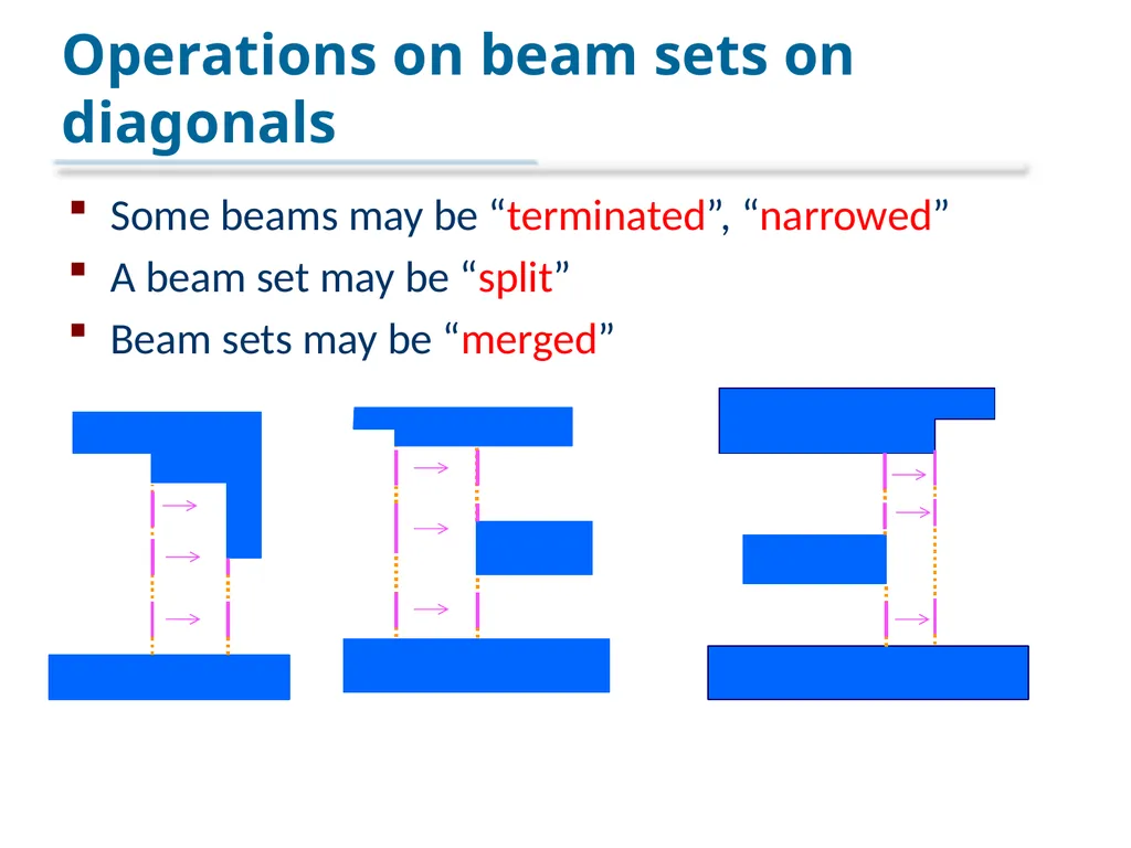
slide23. Operations on beam sets on diagonals Some beams may be “terminated”, “narrowed”
A beam set may be “split”
Beam sets may be “merged”<br>
slide24. Thank you!<br>
Valentin Polishchuk, Linköping University
Mikko Sysikaski, Google Zurich
Haitao Wang, Utah State University
ICALP 2015<br>
slide2. A general polygonal domain Input:
a simple polygon P with some polygons (holes or obstacles) inside, and two points s and t
Output: a path from s to t in P s t<br>
slide3. Minimum-link paths Making a turn in the s-t path is too “expensive”
Output: a minimum-link path from s to t
an s-t path of minimum number of edges (links) s t<br>
slide4. The rectilinear case of minimum-link path problem Each polygon edge is either horizontal or vertical
Each edge of the sought s-t path is also either horizontal or vertical s t<br>
slide5. The rectilinear minimum-link path problem Input: a rectilinear domain P of n vertices and h holes, and s and t
Output: a rectilinear minimum-link s-t path s t n = 39
h = 3<br>
slide6. Previous work and our result The general case
O(n2 α(n) log2 n) time, Mitchell, Rote, and Woeginger 92’
The rectilinear case
O(n log n) time and O(n log n) space, Imai and Asano 86’
O(n log n) time and O(n) space, SSO 87’, DN 91’, MPS 14’
Ω(n + h log h) time lower bound, DN91’, MSD 00’
Our result:
O(n + h log h) time and O(n) space, with a given triangulation of P
triangulating P
O(n + h log1+ε h) time, Bar-Yehuda and Chazelle 94’<br>
slide7. Our result: answering single-source queries Build a data structure in O(n + h log h) time and O(n) space for s, to answer the queries:
given any query point t,
compute the link distance (the number of links of the rectilinear minimum-link s-t path) in O(log n) time
report the actual path in additional time linear in the link distance<br>
slide8. Outline The previous work: Das and Narasimhan, 91’
Our improvement based on their work<br>
slide9. Four types of rectilinear paths Any rectilinear s-t path can be
a vertical-start-vertical-end path, or v-v path
a vertical-start-horizontal-end path, or v-h path
a horizontal-start-vertical-end path, or h-v path
a horizontal-start-horizontal-end path, or h-h path t s t s t s t s v-v path v-h path h-v path h-h path<br>
slide10. Computing a minimum-link path Compute the four paths:
a minimum-link v-v path
a minimum-link v-h path
a minimum-link h-v path
a minimum-link h-h path
Return the one with the minimum link distance as the solution by a v-v link distance map by a v-h map by an h-v map by an h-h map<br>
slide11. Computing a v-v map The vertical decomposition of P, VD(P)
Extend each vertical edge until the boundary of P
Each extension segment is called a diagonal
Computing VD(P) is equivalent to triangulating P<br>
slide12. Computing a v-v map (cont.) VD(P) is our v-v map. Why?
Observation: For each cell, all points in the cell have the same v-v link distance to s s t<br>
slide13. Computing a v-v map (cont.) Label each cell with its v-v link distance to s s 3 3 3 3 3 3 5 5 5 5 5 5 5 5 5 5 5 5 7 7 t 1 3 3<br>
slide14. Labelling the diagonals (the vertical extensions) Initially, label the diagonal ds through s by 1
Put a light source on the entire ds generating light beams towards leftwards and rightwards
any diagonals illuminated by ds will get label 3 3 5<br>
slide15. The algorithm in the previous work In the i-th round, for i = 0, 1, 2, 3…..
Finds a set Vi of diagonals and label them 2i + 1
What is Vi ?
If we put light sources on all diagonals of Vi-1, then Vi consists of all new diagonals that can be illuminated
Two sweeping procedures: left-sweep and right-sweep
A heap is used to guide the sweeping such that the diagonals are processed by their x-coordinates
The sweeping is controlled in a global manner
O(n log n) time in total<br>
slide16. Our improvement: using a corridor structure Consider the dual graph G of the VD(P)
Keep removing the degree-one nodes from G
Keep contracting the degree-two nodes<br>
slide17. Our improvement: using a corridor structure The remaining graph G’ is called “corridor graph”
Each vertex of G’ corresponds to a “junction cell”
Each edge of G’ corresponds to a “corridor”<br>
slide18. Our improvement: using a corridor structure (cont.) Each corridor is a simple rectilinear polygon
Each corridor has two doors connecting with its neighboring junction cells<br>
slide19. Our improvement: using a corridor structure (cont.) There are O(h) junction cells and O(h) corridors
Incorporating the source point s
s is considered as a special vertex of the corridor graph
The diagonal ds is considered as a special junction cell s<br>
slide20. Our algorithm – an overview We use the same sweeping approach as before with the following differences
The sweeping in the junction cells is controlled in a global manner, the same as before
Once the sweeping enters into a corridor C through one of its doors, we sweep C in a local manner
What is the benefit?
The global sweeping is only on junction cells
There are only O(h) junction cells O(h log h) time
The local sweeping in each corridor can be processed in linear time since it is a simple polygon
The total size of all corridors is O(n) O(n) time<br>
slide21. Our algorithm – a demonstration s 1 5 5 3 3 3 3<br>
slide22. The sweeping in corridors Suppose there are h1 beams entering a corridor C through a door, and h2 beams leaving C through the other door after the sweeping
Our algorithm runs in O(|C| + (h1 – h2 ) log h1) time
The sum of the first term in the entire algorithm is O(n)
The sum of the second term is O(h log h) h1 = 5 h2 = 2 C<br>
slide23. Operations on beam sets on diagonals Some beams may be “terminated”, “narrowed”
A beam set may be “split”
Beam sets may be “merged”<br>
slide24. Thank you!<br>