
ANIMAL GENETICS & BREEDING UNIT – II Principles of


Description: ANIMAL GENETICS BREEDING UNIT II Principles of Animal Population Genetics Quantitative Genetics: Values Means Dr K G Mandal Department of Animal Genetics Breeding Bihar Veterinary College, Patna Bihar Animal Sciences University,
Related Topics
Download Presentation
"ANIMAL GENETICS & BREEDING UNIT – II Principles of" is the property of its rightful owner. Permission is granted to download and print the materials on this website for personal, non-commercial use only, and to display it on your personal computer provided you do not modify the materials and that you retain all copyright notices contained in the materials. By downloading content from our website, you accept the terms of this agreement.
Presentation Transcript
slide1. ANIMAL GENETICS & BREEDING
UNIT – II
Principles of Animal & Population Genetics
Quantitative Genetics: Values & Means
Dr K G Mandal
Department of Animal Genetics & Breeding
Bihar Veterinary College, Patna
Bihar Animal Sciences University, Patna<br>
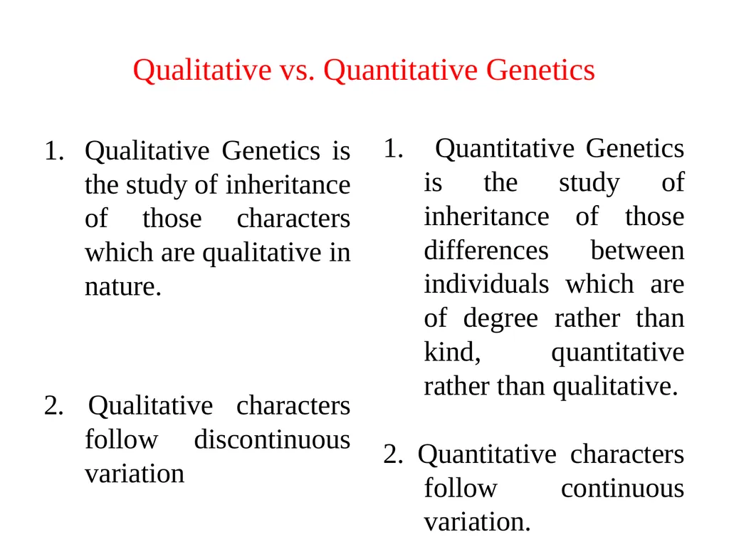
slide2. Qualitative vs. Quantitative Genetics Qualitative Genetics is the study of inheritance of those characters which are qualitative in nature.
2. Qualitative characters follow discontinuous variation Quantitative Genetics is the study of inheritance of those differences between individuals which are of degree rather than kind, quantitative rather than qualitative.
2. Quantitative characters follow continuous variation.<br>
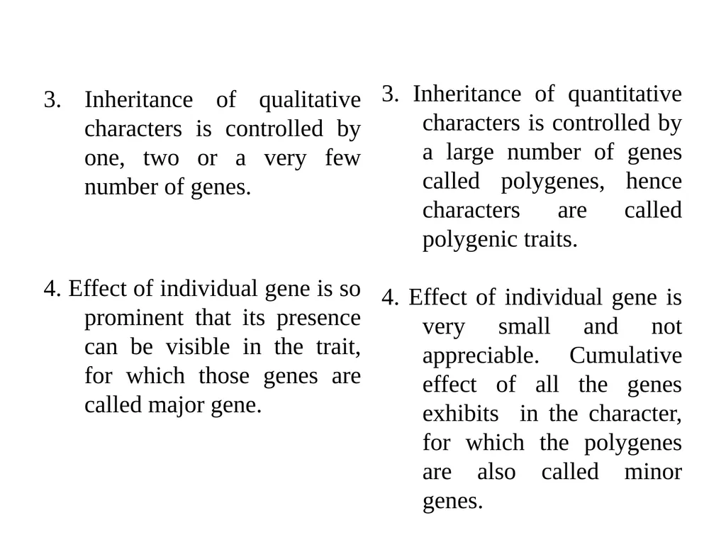
slide3. 3. Inheritance of qualitative characters is controlled by one, two or a very few number of genes.
4. Effect of individual gene is so prominent that its presence can be visible in the trait, for which those genes are called major gene. 3. Inheritance of quantitative characters is controlled by a large number of genes called polygenes, hence characters are called polygenic traits.
4. Effect of individual gene is very small and not appreciable. Cumulative effect of all the genes exhibits in the character, for which the polygenes are also called minor genes.<br>
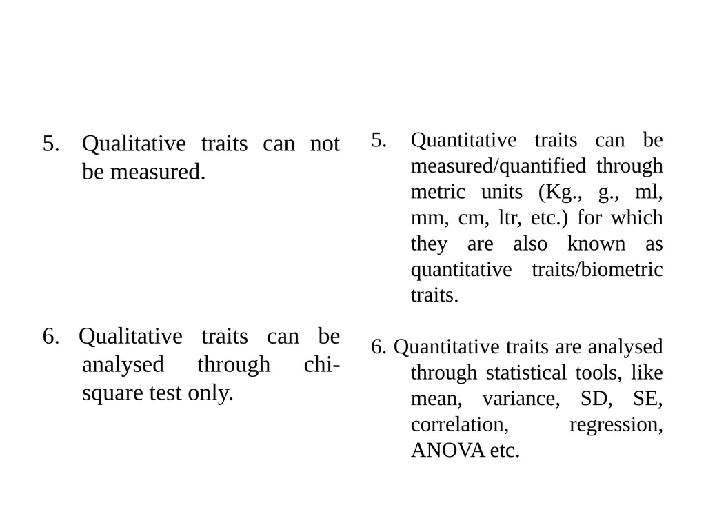
slide4. Qualitative traits can not be measured.
6. Qualitative traits can be analysed through chi-square test only. Quantitative traits can be measured/quantified through metric units (Kg., g., ml, mm, cm, ltr, etc.) for which they are also known as quantitative traits/biometric traits.
6. Quantitative traits are analysed through statistical tools, like mean, variance, SD, SE, correlation, regression, ANOVA etc.<br>
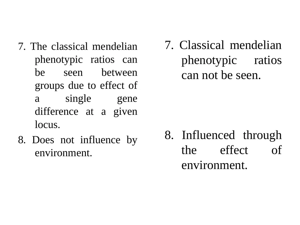
slide5. 7. The classical mendelian phenotypic ratios can be seen between groups due to effect of a single gene difference at a given locus.
8. Does not influence by environment. 7. Classical mendelian phenotypic ratios can not be seen.
8. Influenced through the effect of environment.<br>
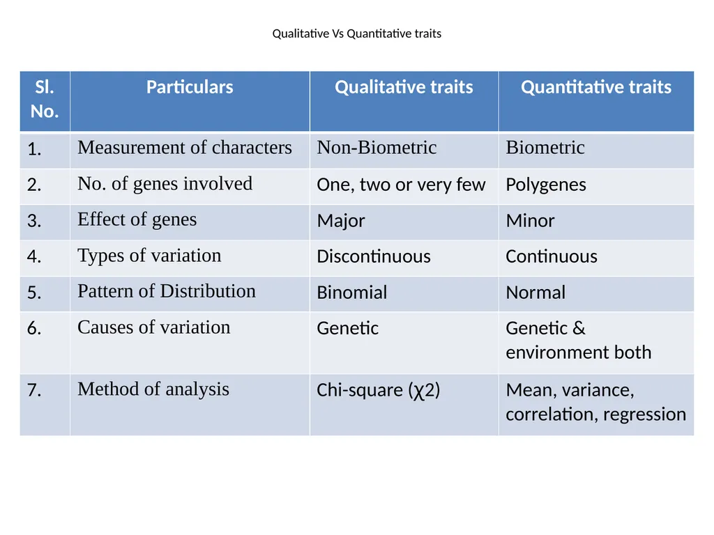
slide6. Qualitative Vs Quantitative traits<br>
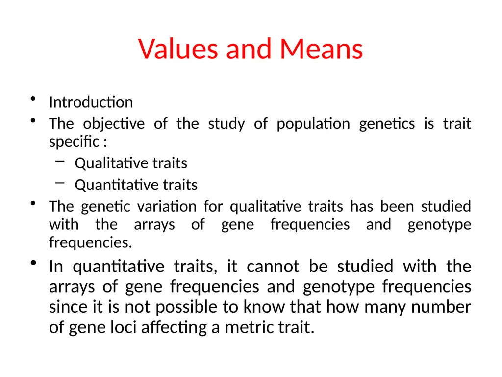
slide7. Values and Means Introduction
The objective of the study of population genetics is trait specific :
Qualitative traits
Quantitative traits
The genetic variation for qualitative traits has been studied with the arrays of gene frequencies and genotype frequencies.
In quantitative traits, it cannot be studied with the arrays of gene frequencies and genotype frequencies since it is not possible to know that how many number of gene loci affecting a metric trait.<br>
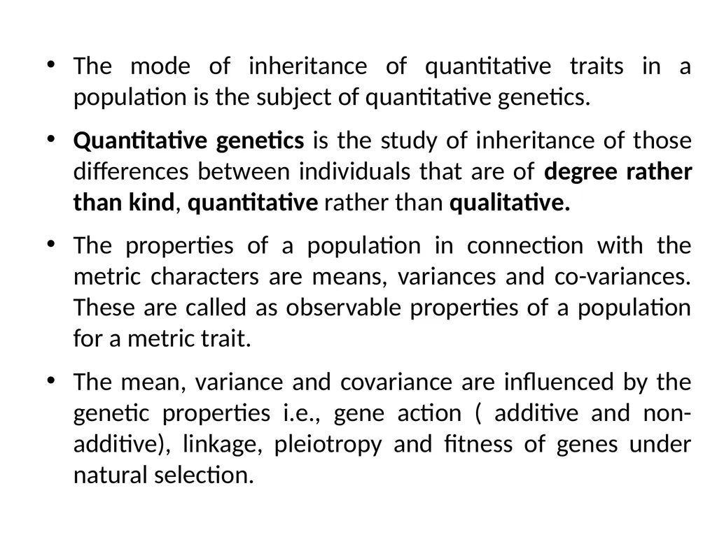
slide8. The mode of inheritance of quantitative traits in a population is the subject of quantitative genetics.
Quantitative genetics is the study of inheritance of those differences between individuals that are of degree rather than kind, quantitative rather than qualitative.
The properties of a population in connection with the metric characters are means, variances and co-variances. These are called as observable properties of a population for a metric trait.
The mean, variance and covariance are influenced by the genetic properties i.e., gene action ( additive and non-additive), linkage, pleiotropy and fitness of genes under natural selection.<br>
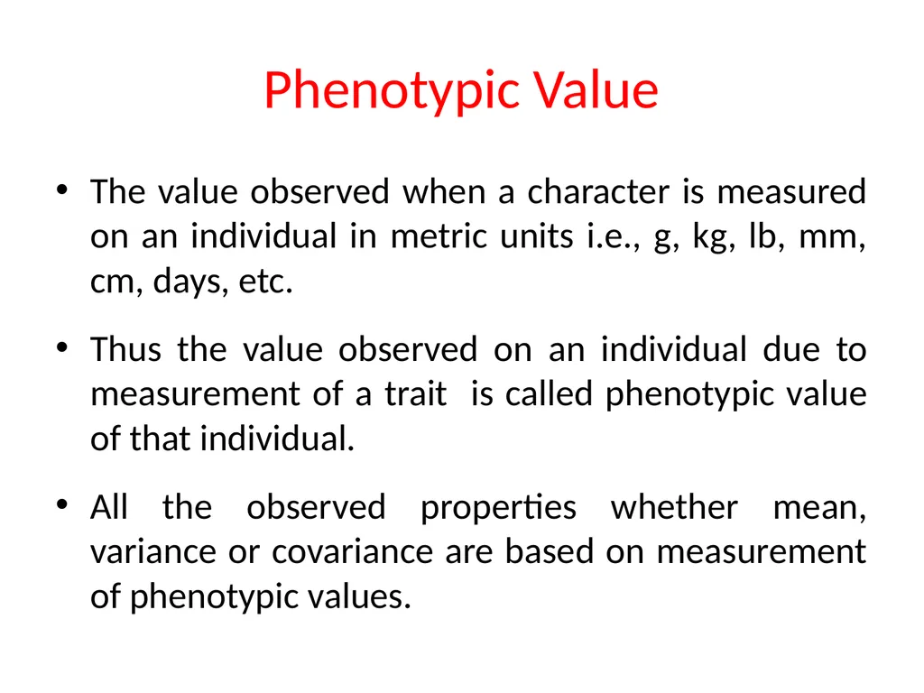
slide9. Phenotypic Value The value observed when a character is measured on an individual in metric units i.e., g, kg, lb, mm, cm, days, etc.
Thus the value observed on an individual due to measurement of a trait is called phenotypic value of that individual.
All the observed properties whether mean, variance or covariance are based on measurement of phenotypic values.<br>
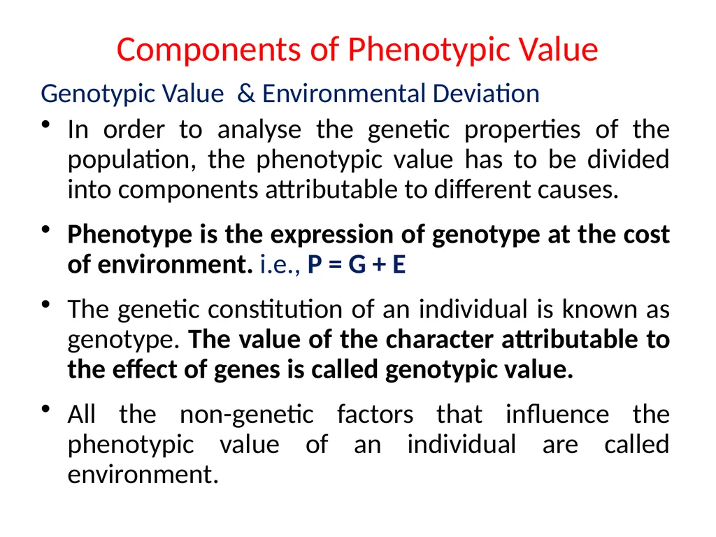
slide10. Components of Phenotypic Value Genotypic Value & Environmental Deviation
In order to analyse the genetic properties of the population, the phenotypic value has to be divided into components attributable to different causes.
Phenotype is the expression of genotype at the cost of environment. i.e., P = G + E
The genetic constitution of an individual is known as genotype. The value of the character attributable to the effect of genes is called genotypic value.
All the non-genetic factors that influence the phenotypic value of an individual are called environment.<br>
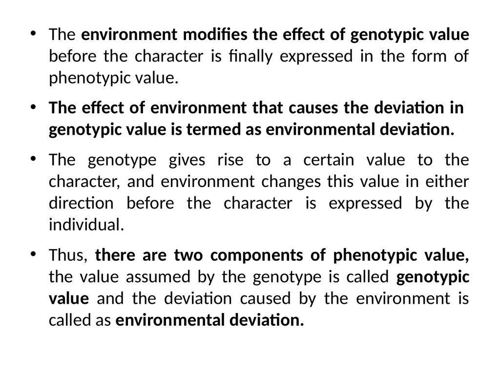
slide11. The environment modifies the effect of genotypic value before the character is finally expressed in the form of phenotypic value.
The effect of environment that causes the deviation in genotypic value is termed as environmental deviation.
The genotype gives rise to a certain value to the character, and environment changes this value in either direction before the character is expressed by the individual.
Thus, there are two components of phenotypic value, the value assumed by the genotype is called genotypic value and the deviation caused by the environment is called as environmental deviation.<br>
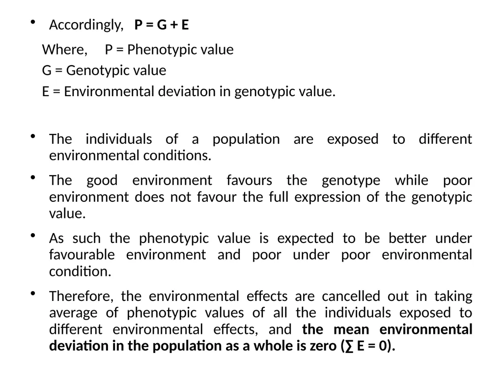
slide12. Accordingly, P = G + E
Where, P = Phenotypic value
G = Genotypic value
E = Environmental deviation in genotypic value.
The individuals of a population are exposed to different environmental conditions.
The good environment favours the genotype while poor environment does not favour the full expression of the genotypic value.
As such the phenotypic value is expected to be better under favourable environment and poor under poor environmental condition.
Therefore, the environmental effects are cancelled out in taking average of phenotypic values of all the individuals exposed to different environmental effects, and the mean environmental deviation in the population as a whole is zero (∑ E = 0).<br>
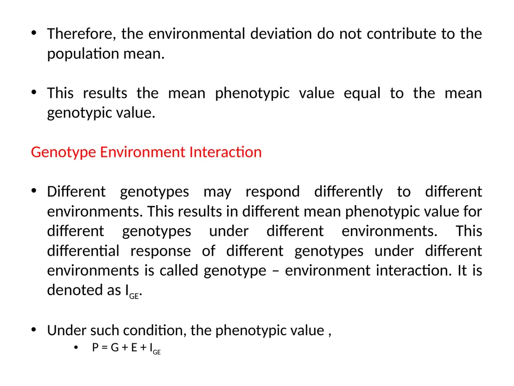
slide13. Therefore, the environmental deviation do not contribute to the population mean.
This results the mean phenotypic value equal to the mean genotypic value.
Genotype Environment Interaction
Different genotypes may respond differently to different environments. This results in different mean phenotypic value for different genotypes under different environments. This differential response of different genotypes under different environments is called genotype – environment interaction. It is denoted as IGE.
Under such condition, the phenotypic value ,
P = G + E + IGE<br>
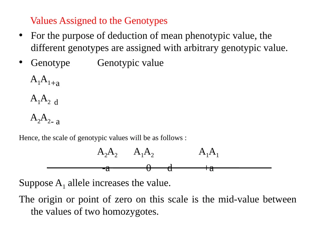
slide14. Values Assigned to the Genotypes
For the purpose of deduction of mean phenotypic value, the different genotypes are assigned with arbitrary genotypic value.
Genotype Genotypic value
A1A1 +a
A1A2 d
A2A2 - a
Hence, the scale of genotypic values will be as follows :
A2A2 A1A2 A1A1
-a 0 d +a
Suppose A1 allele increases the value.
The origin or point of zero on this scale is the mid-value between the values of two homozygotes.<br>
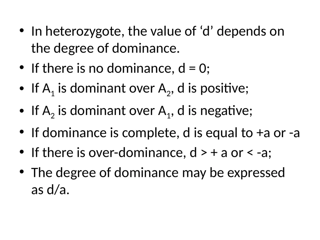
slide15. In heterozygote, the value of ‘d’ depends on the degree of dominance.
If there is no dominance, d = 0;
If A1 is dominant over A2, d is positive;
If A2 is dominant over A1, d is negative;
If dominance is complete, d is equal to +a or -a
If there is over-dominance, d > + a or < -a;
The degree of dominance may be expressed as d/a.<br>
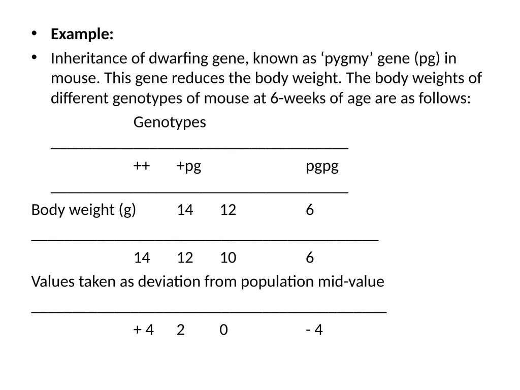
slide16. Example:
Inheritance of dwarfing gene, known as ‘pygmy’ gene (pg) in mouse. This gene reduces the body weight. The body weights of different genotypes of mouse at 6-weeks of age are as follows:
Genotypes ____________________________________
++ +pg pgpg ____________________________________
Body weight (g) 14 12 6
__________________________________________
14 12 10 6
Values taken as deviation from population mid-value
___________________________________________
+ 4 2 0 - 4<br>
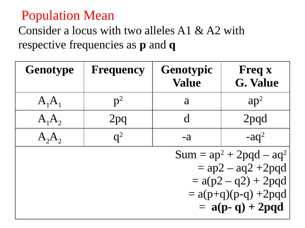
slide17. Population Mean Consider a locus with two alleles A1 & A2 with respective frequencies as p and q<br>
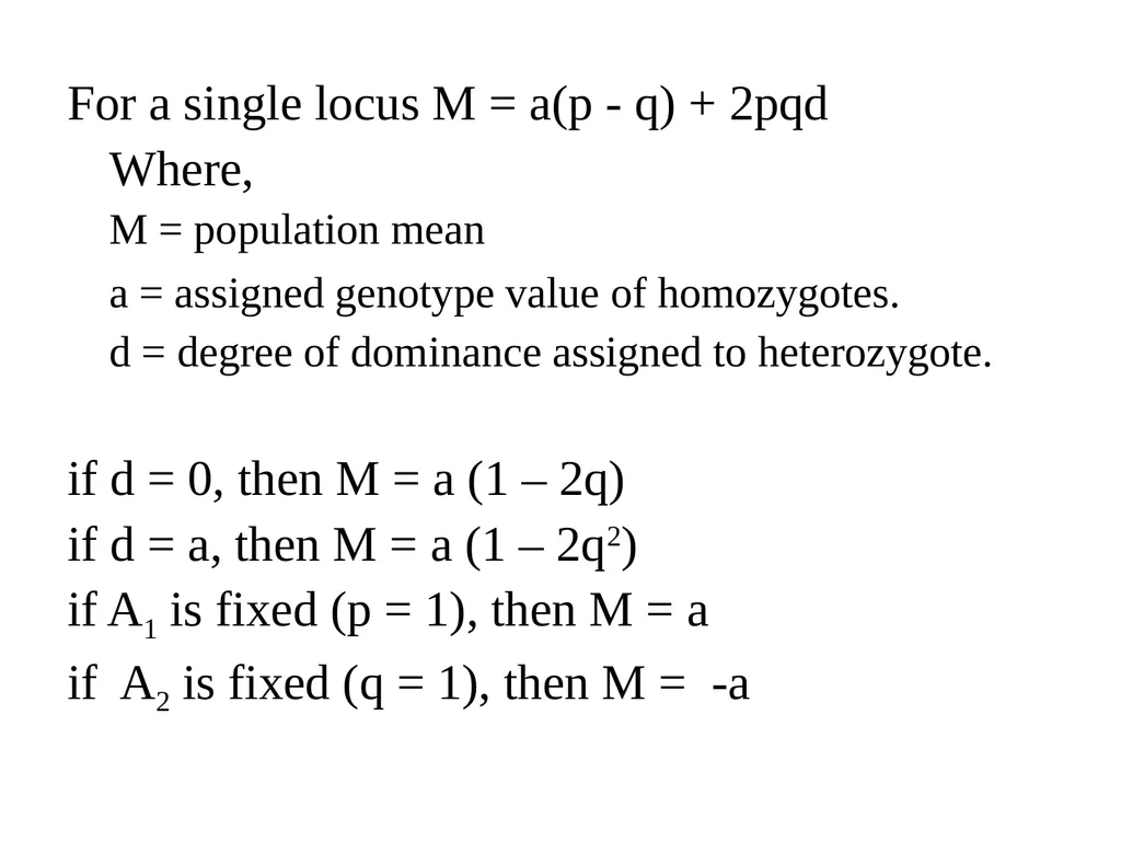
slide18. For a single locus M = a(p - q) + 2pqd
Where,
M = population mean
a = assigned genotype value of homozygotes.
d = degree of dominance assigned to heterozygote.
if d = 0, then M = a (1 – 2q)
if d = a, then M = a (1 – 2q2)
if A1 is fixed (p = 1), then M = a
if A2 is fixed (q = 1), then M = -a<br>
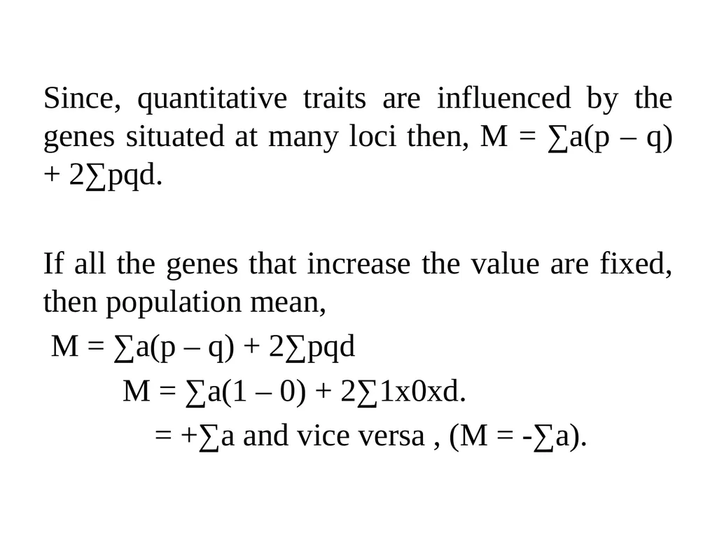
slide19. Since, quantitative traits are influenced by the genes situated at many loci then, M = ∑a(p – q) + 2∑pqd.
If all the genes that increase the value are fixed, then population mean,
M = ∑a(p – q) + 2∑pqd
M = ∑a(1 – 0) + 2∑1x0xd.
= +∑a and vice versa , (M = -∑a).<br>
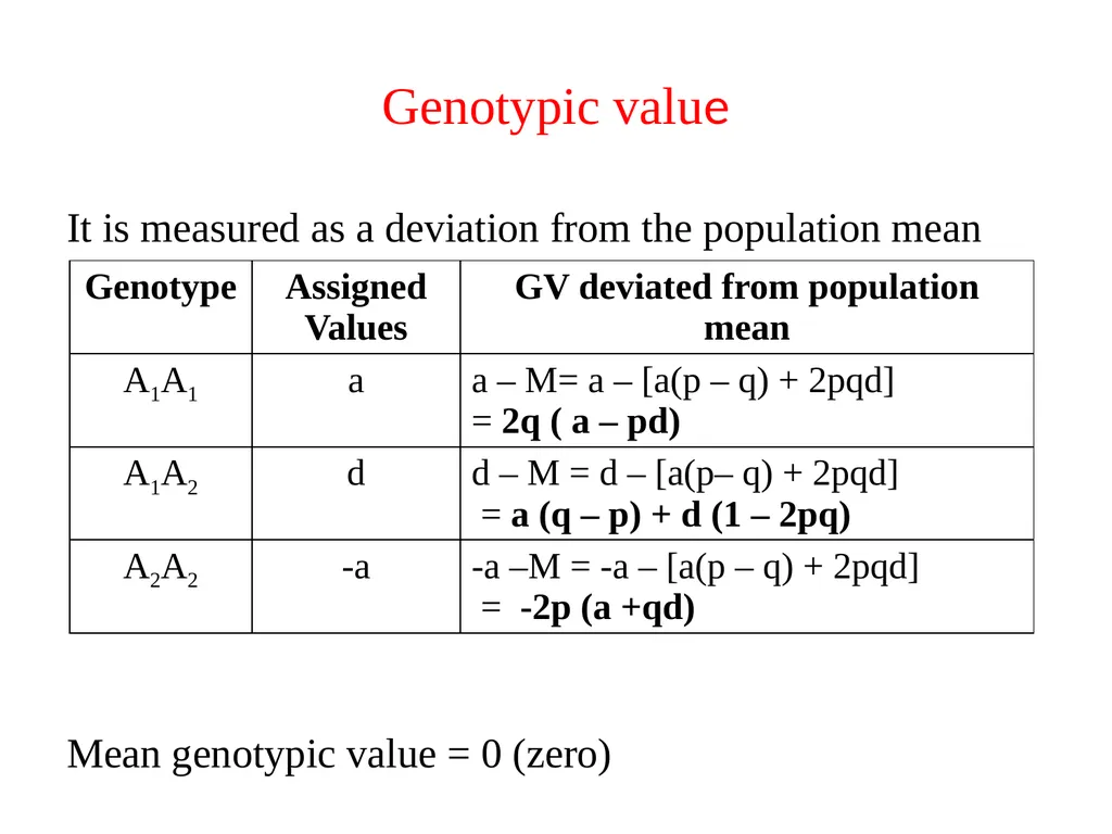
slide20. Genotypic value It is measured as a deviation from the population mean
Mean genotypic value = 0 (zero)<br>
slide21. Genotypic value of A1A1
= a – [a(p – q) + 2pqd]
= a(1 – p +q) – 2pqd
= a(p + q – p +q) – 2pqd
= a(2q) – 2pqd
= 2q(a – pd)
Genotypic value of A2A2
= -a - [a(p – q) + 2pqd]
= -a(1 + p – q) - 2pqd
= -a(p + q + p – q) - 2pqd
= -a(2p) - 2pqd
= - 2p(a + qd)<br>
slide22. Mean Genotypic Value
Since the genotypic values are taken as deviation from the population mean, the mean genotypic value of the population would be zero.
The mean genotypic value = sum of product between genotypic value and frequency of respective genotypes.
Thus, mean genotypic value
= p2[2q(a – pd)] + 2pq[a(q – p) + d(1 – 2pq] + q2[ - 2p(a + qd)]
= 2p2q(a – pd) + 2pqa(q – p) + 2pqd – 4p2q2d – 2pq2a – 2pq3d
= 2p2qa – 2p3qd + 2pq2a – 2p2qa + 2pqd – 4p2q2d – 2pq2a - 2pq3d
= – 2p3qd + 2pqd – 4p2q2d – 2pq3d
= - 2pqd[p2 – 1 + 2pq + q2]
= -2pqd[ p2 + 2pq +q2 – 1]
= -2pqd[1 – 1]
= 0<br>
slide23. THANK YOU<br>
slide2. Qualitative vs. Quantitative Genetics Qualitative Genetics is the study of inheritance of those characters which are qualitative in nature.
2. Qualitative characters follow discontinuous variation Quantitative Genetics is the study of inheritance of those differences between individuals which are of degree rather than kind, quantitative rather than qualitative.
2. Quantitative characters follow continuous variation.<br>
slide3. 3. Inheritance of qualitative characters is controlled by one, two or a very few number of genes.
4. Effect of individual gene is so prominent that its presence can be visible in the trait, for which those genes are called major gene. 3. Inheritance of quantitative characters is controlled by a large number of genes called polygenes, hence characters are called polygenic traits.
4. Effect of individual gene is very small and not appreciable. Cumulative effect of all the genes exhibits in the character, for which the polygenes are also called minor genes.<br>
slide4. Qualitative traits can not be measured.
6. Qualitative traits can be analysed through chi-square test only. Quantitative traits can be measured/quantified through metric units (Kg., g., ml, mm, cm, ltr, etc.) for which they are also known as quantitative traits/biometric traits.
6. Quantitative traits are analysed through statistical tools, like mean, variance, SD, SE, correlation, regression, ANOVA etc.<br>
slide5. 7. The classical mendelian phenotypic ratios can be seen between groups due to effect of a single gene difference at a given locus.
8. Does not influence by environment. 7. Classical mendelian phenotypic ratios can not be seen.
8. Influenced through the effect of environment.<br>
slide6. Qualitative Vs Quantitative traits<br>
slide7. Values and Means Introduction
The objective of the study of population genetics is trait specific :
Qualitative traits
Quantitative traits
The genetic variation for qualitative traits has been studied with the arrays of gene frequencies and genotype frequencies.
In quantitative traits, it cannot be studied with the arrays of gene frequencies and genotype frequencies since it is not possible to know that how many number of gene loci affecting a metric trait.<br>
slide8. The mode of inheritance of quantitative traits in a population is the subject of quantitative genetics.
Quantitative genetics is the study of inheritance of those differences between individuals that are of degree rather than kind, quantitative rather than qualitative.
The properties of a population in connection with the metric characters are means, variances and co-variances. These are called as observable properties of a population for a metric trait.
The mean, variance and covariance are influenced by the genetic properties i.e., gene action ( additive and non-additive), linkage, pleiotropy and fitness of genes under natural selection.<br>
slide9. Phenotypic Value The value observed when a character is measured on an individual in metric units i.e., g, kg, lb, mm, cm, days, etc.
Thus the value observed on an individual due to measurement of a trait is called phenotypic value of that individual.
All the observed properties whether mean, variance or covariance are based on measurement of phenotypic values.<br>
slide10. Components of Phenotypic Value Genotypic Value & Environmental Deviation
In order to analyse the genetic properties of the population, the phenotypic value has to be divided into components attributable to different causes.
Phenotype is the expression of genotype at the cost of environment. i.e., P = G + E
The genetic constitution of an individual is known as genotype. The value of the character attributable to the effect of genes is called genotypic value.
All the non-genetic factors that influence the phenotypic value of an individual are called environment.<br>
slide11. The environment modifies the effect of genotypic value before the character is finally expressed in the form of phenotypic value.
The effect of environment that causes the deviation in genotypic value is termed as environmental deviation.
The genotype gives rise to a certain value to the character, and environment changes this value in either direction before the character is expressed by the individual.
Thus, there are two components of phenotypic value, the value assumed by the genotype is called genotypic value and the deviation caused by the environment is called as environmental deviation.<br>
slide12. Accordingly, P = G + E
Where, P = Phenotypic value
G = Genotypic value
E = Environmental deviation in genotypic value.
The individuals of a population are exposed to different environmental conditions.
The good environment favours the genotype while poor environment does not favour the full expression of the genotypic value.
As such the phenotypic value is expected to be better under favourable environment and poor under poor environmental condition.
Therefore, the environmental effects are cancelled out in taking average of phenotypic values of all the individuals exposed to different environmental effects, and the mean environmental deviation in the population as a whole is zero (∑ E = 0).<br>
slide13. Therefore, the environmental deviation do not contribute to the population mean.
This results the mean phenotypic value equal to the mean genotypic value.
Genotype Environment Interaction
Different genotypes may respond differently to different environments. This results in different mean phenotypic value for different genotypes under different environments. This differential response of different genotypes under different environments is called genotype – environment interaction. It is denoted as IGE.
Under such condition, the phenotypic value ,
P = G + E + IGE<br>
slide14. Values Assigned to the Genotypes
For the purpose of deduction of mean phenotypic value, the different genotypes are assigned with arbitrary genotypic value.
Genotype Genotypic value
A1A1 +a
A1A2 d
A2A2 - a
Hence, the scale of genotypic values will be as follows :
A2A2 A1A2 A1A1
-a 0 d +a
Suppose A1 allele increases the value.
The origin or point of zero on this scale is the mid-value between the values of two homozygotes.<br>
slide15. In heterozygote, the value of ‘d’ depends on the degree of dominance.
If there is no dominance, d = 0;
If A1 is dominant over A2, d is positive;
If A2 is dominant over A1, d is negative;
If dominance is complete, d is equal to +a or -a
If there is over-dominance, d > + a or < -a;
The degree of dominance may be expressed as d/a.<br>
slide16. Example:
Inheritance of dwarfing gene, known as ‘pygmy’ gene (pg) in mouse. This gene reduces the body weight. The body weights of different genotypes of mouse at 6-weeks of age are as follows:
Genotypes ____________________________________
++ +pg pgpg ____________________________________
Body weight (g) 14 12 6
__________________________________________
14 12 10 6
Values taken as deviation from population mid-value
___________________________________________
+ 4 2 0 - 4<br>
slide17. Population Mean Consider a locus with two alleles A1 & A2 with respective frequencies as p and q<br>
slide18. For a single locus M = a(p - q) + 2pqd
Where,
M = population mean
a = assigned genotype value of homozygotes.
d = degree of dominance assigned to heterozygote.
if d = 0, then M = a (1 – 2q)
if d = a, then M = a (1 – 2q2)
if A1 is fixed (p = 1), then M = a
if A2 is fixed (q = 1), then M = -a<br>
slide19. Since, quantitative traits are influenced by the genes situated at many loci then, M = ∑a(p – q) + 2∑pqd.
If all the genes that increase the value are fixed, then population mean,
M = ∑a(p – q) + 2∑pqd
M = ∑a(1 – 0) + 2∑1x0xd.
= +∑a and vice versa , (M = -∑a).<br>
slide20. Genotypic value It is measured as a deviation from the population mean
Mean genotypic value = 0 (zero)<br>
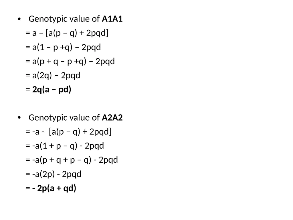
slide21. Genotypic value of A1A1
= a – [a(p – q) + 2pqd]
= a(1 – p +q) – 2pqd
= a(p + q – p +q) – 2pqd
= a(2q) – 2pqd
= 2q(a – pd)
Genotypic value of A2A2
= -a - [a(p – q) + 2pqd]
= -a(1 + p – q) - 2pqd
= -a(p + q + p – q) - 2pqd
= -a(2p) - 2pqd
= - 2p(a + qd)<br>
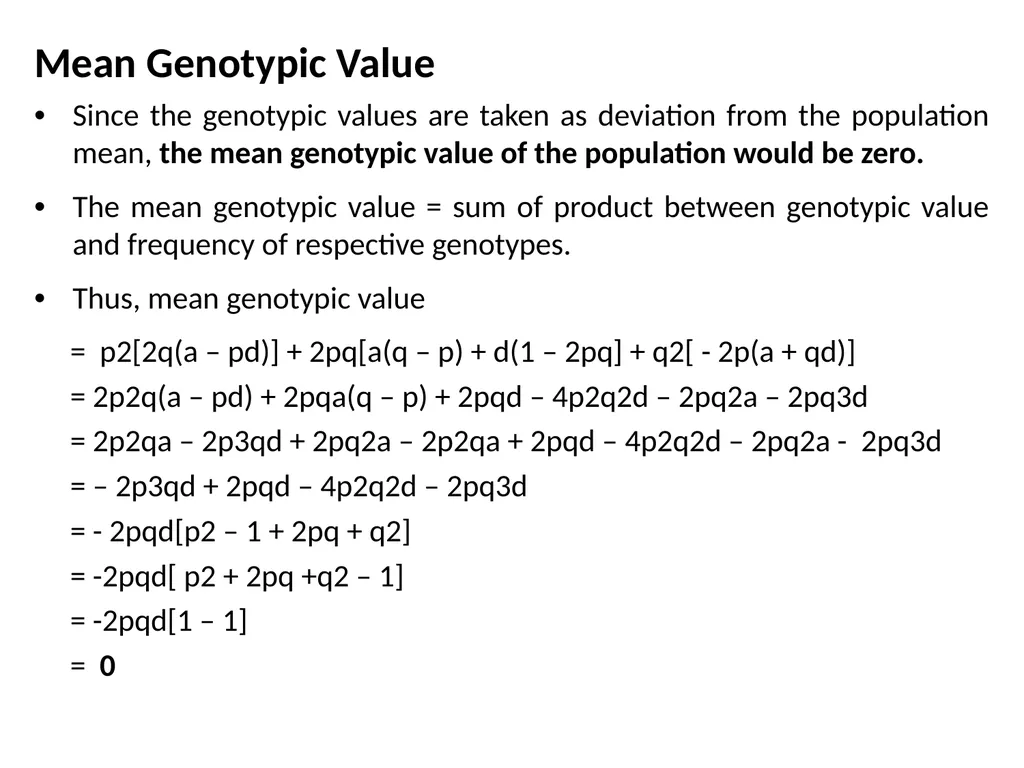
slide22. Mean Genotypic Value
Since the genotypic values are taken as deviation from the population mean, the mean genotypic value of the population would be zero.
The mean genotypic value = sum of product between genotypic value and frequency of respective genotypes.
Thus, mean genotypic value
= p2[2q(a – pd)] + 2pq[a(q – p) + d(1 – 2pq] + q2[ - 2p(a + qd)]
= 2p2q(a – pd) + 2pqa(q – p) + 2pqd – 4p2q2d – 2pq2a – 2pq3d
= 2p2qa – 2p3qd + 2pq2a – 2p2qa + 2pqd – 4p2q2d – 2pq2a - 2pq3d
= – 2p3qd + 2pqd – 4p2q2d – 2pq3d
= - 2pqd[p2 – 1 + 2pq + q2]
= -2pqd[ p2 + 2pq +q2 – 1]
= -2pqd[1 – 1]
= 0<br>
slide23. THANK YOU<br>