Application of Computer in Economics Course:

slide1. Application of Computer in Economics Course: DE-403(ii)

Course teacher
Dr. Sanatan Nayak

Dept. of Economics,
B.B. Ambedkar University
Rae Bareli Road, Lucknow-25<br>
slide2. Contents of Introductions Definitions
Features or characteristics
Basic computer Organization/ Components
Evolution<br>
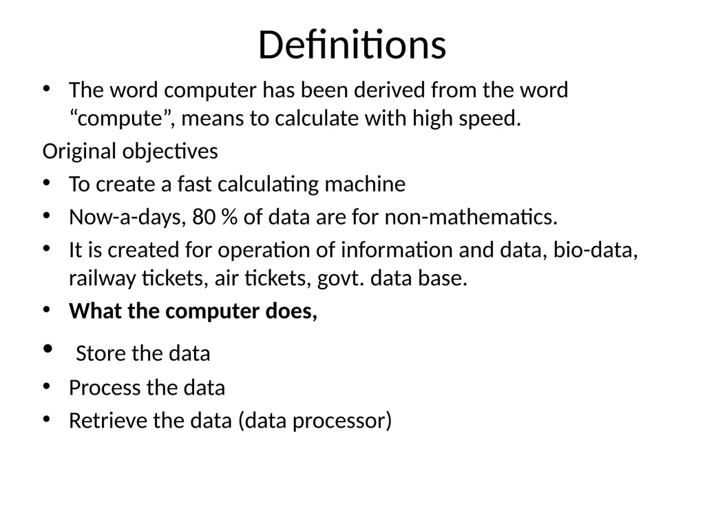
slide3. Definitions The word computer has been derived from the word “compute”, means to calculate with high speed.
Original objectives
To create a fast calculating machine
Now-a-days, 80 % of data are for non-mathematics.
It is created for operation of information and data, bio-data, railway tickets, air tickets, govt. data base.
What the computer does,
Store the data
Process the data
Retrieve the data (data processor)<br>
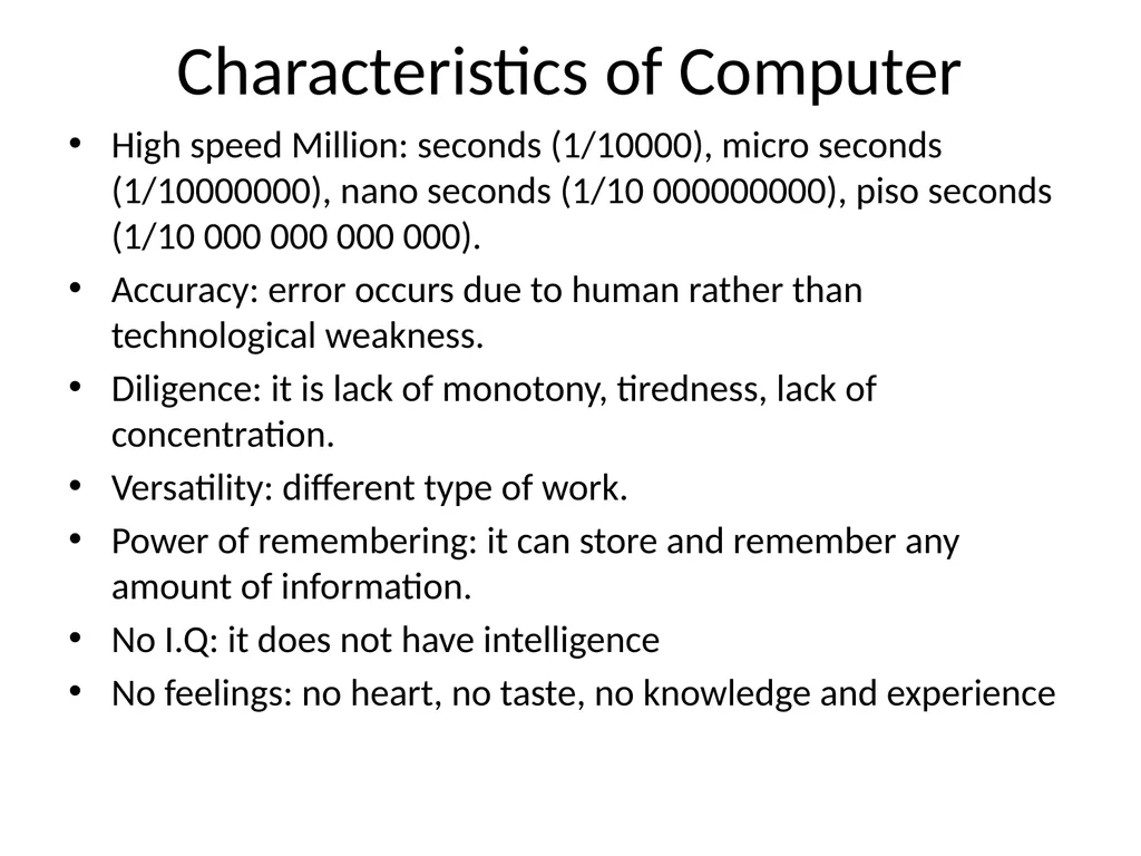
slide4. Characteristics of Computer High speed Million: seconds (1/10000), micro seconds (1/10000000), nano seconds (1/10 000000000), piso seconds (1/10 000 000 000 000).
Accuracy: error occurs due to human rather than technological weakness.
Diligence: it is lack of monotony, tiredness, lack of concentration.
Versatility: different type of work.
Power of remembering: it can store and remember any amount of information.
No I.Q: it does not have intelligence
No feelings: no heart, no taste, no knowledge and experience<br>
slide5. Evolution of Computer Necessary is the mother of invention.
The earliest one that qualifies “abaccus” or “soroban”. It was invented in 600 B.C.
It does only addition, subtraction with little speed.
Manual Calculating device: John Napier’s Card Board- 17th century and updated in 1890 AD.
First mechanical machine by Blair Pascal in 1642 AD.
Baron Gottfried: German’s first calculator for multiplication.
Key Board originated in 1880 AD in USA.
Herman Hollerith: Punched cards are extensively used a input media in modern digital computer.<br>
slide6. Basic Computer’s Organization Five important operations:
Inputting
Storing
Processing
Outputting
Controlling
Therefore, five important functional units or blocks.
Input Unit:
Data and information must be given through outside device.
Through Key Board
All the data and instruction are transformed into binary codes/acceptable form, those are saved in primary memory.
It supplies the converted instructions and data to the computer system for further processing.<br>
slide7. Basic Computer’s Organization cont …. 2. Output Unit:
It is reverse of input Unit
It accept the result produced by the computer, which are in coded form and can not be easily understand by us.
It convert from binary form to the human acceptable form.
It is designed to the external environment through printer etc.
It supplies information and results of the computer to the outside world.
3. Storage Unit:
All the data and instructions to be stored and kept for processing (received from input device)
It stores the intermediate results for processing.
Final results of processing before these results are released to be an output device.<br>
slide8. Basic Computer’s Organization cont …. 4. Arithmetic Logic Unit
It is the place where actual execution of instruction are taken place.
All the calculations are performed and all decisions are made in ALU
All data and instructions are stored in the primary storage prior to the processing are transferred as and when needed to ALU.
Intermediate results are generated in the ALU are temporarily transferred back to primary storage.
All the ALU are designed to perform the four basic arithmatic operations, +, -, X, / and all the logic operation, / , >, <,<br>
slide9. Basic Computer’s Organization cont …. 5. Control Unit:
It is central nervous system in the computer.
It abtain instructions from the programme stored in main memory, interpret the instructions and issues signal that cause other units of the system to execute.
It acts as selection, interpretation and execution of instruction.
Central Processing Units (CPU)
CU + ALU = CPU<br>
slide10. References P.K. Sinha (latest), Computer Fundamentals, BPB Publications, New Delhi.<br>
slide11. Goals of the chapter This chapter deals with
Various Generations Computers
Types of computers<br>
slide12. Generations of Computers Classifications of generations is based on
Development of hard wares in the computers
Development of soft wares and its applications<br>
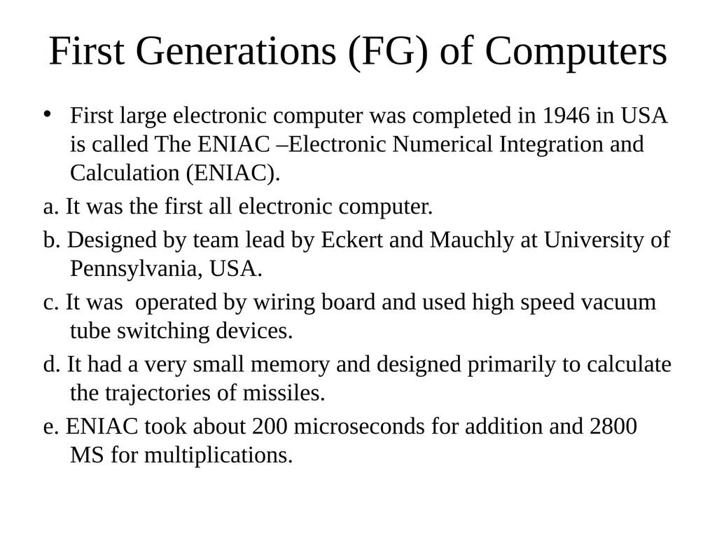
slide13. First Generations (FG) of Computers First large electronic computer was completed in 1946 in USA is called The ENIAC –Electronic Numerical Integration and Calculation (ENIAC).
a. It was the first all electronic computer.
b. Designed by team lead by Eckert and Mauchly at University of Pennsylvania, USA.
c. It was operated by wiring board and used high speed vacuum tube switching devices.
d. It had a very small memory and designed primarily to calculate the trajectories of missiles.
e. ENIAC took about 200 microseconds for addition and 2800 MS for multiplications.<br>
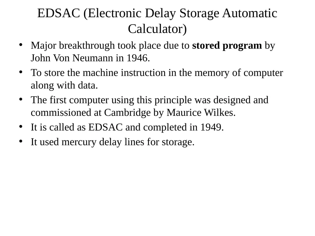
slide14. EDSAC (Electronic Delay Storage Automatic Calculator) Major breakthrough took place due to stored program by John Von Neumann in 1946.
To store the machine instruction in the memory of computer along with data.
The first computer using this principle was designed and commissioned at Cambridge by Maurice Wilkes.
It is called as EDSAC and completed in 1949.
It used mercury delay lines for storage.<br>
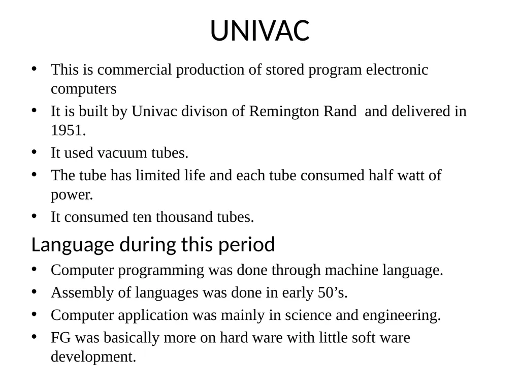
slide15. UNIVAC This is commercial production of stored program electronic computers
It is built by Univac divison of Remington Rand and delivered in 1951.
It used vacuum tubes.
The tube has limited life and each tube consumed half watt of power.
It consumed ten thousand tubes.
Language during this period
Computer programming was done through machine language.
Assembly of languages was done in early 50’s.
Computer application was mainly in science and engineering.
FG was basically more on hard ware with little soft ware development.<br>
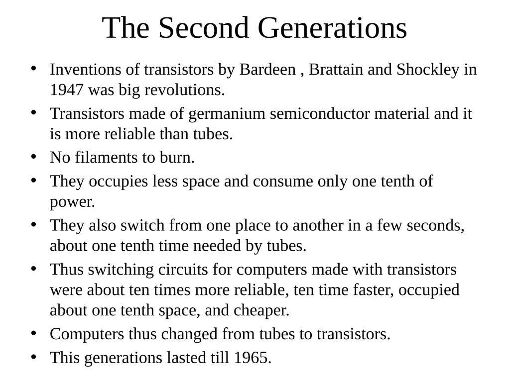
slide16. The Second Generations Inventions of transistors by Bardeen , Brattain and Shockley in 1947 was big revolutions.
Transistors made of germanium semiconductor material and it is more reliable than tubes.
No filaments to burn.
They occupies less space and consume only one tenth of power.
They also switch from one place to another in a few seconds, about one tenth time needed by tubes.
Thus switching circuits for computers made with transistors were about ten times more reliable, ten time faster, occupied about one tenth space, and cheaper.
Computers thus changed from tubes to transistors.
This generations lasted till 1965.<br>
slide17. SG Continu……. Another major invention was magnetic cores of storage.
Magnetic cores are tiny rings (0.05 cm diameter) made of ferrite and can be magnetized in either clock wise or anti-clock wise direction.
Magnetic cores were used to construct large random access memories.
Memory capacity in SG was about 100 KB
Magnetic disk storage was developed during this period.
Due to development of Large Memories
Development of high level languages, FORTRAN, COBOL, Algol, SNOWBOL were developed.
With higher speed of CPU, disk storage, operating systems were developed.
Good batch operating system particularly 7000 series computers emerged during the SG.<br>
slide18. SG Continu……. Rapid development of computers due to development of business and industry (80%).
A number of application operation research such as linear programming, critical path methods (CPM), simulation were used in computers.
New professions in computing such as systems analysis and programmers emerged during the second generations
Academic programmes in computer sciences were also initiated.<br>
slide19. The Third Generations (TG) The TG began in 1965 with germanium transistors replaced by silicon transistors.
Integrated circuits, circuits consist of transistors, resistors and capacitors grown on single chip of silicon eliminating wired interconnection between components emerged.
From small scale circuits to medium scale circuit of 100 transistors per chips developed.
Switching speed of transistors went up by a factors of 10 times.
Reliability increased by factor of 10.
Power dissipation increased by factor of 10
Size also reduce by factor of 10
Powerful CPU with carrying capacity of 1 million instructions per seconds.<br>
slide20. (TG) Conti…… There were significant improvements in design of magnetic core meories.
The size of main memories reached about 4 MB.
Magnetic disk technology improved rapidly.
100 MB drive became feasible.
Time shared operating system was developed (combination of high capacity memory, powerful CPU, large disk memories).
Many important online systems became feasible.
Dynamic production control system developed.
Airline reservation, interactive query systems and real time closed loop process control system were developed.
Integrated data base management system was developed.<br>
slide21. (TG) Conti…… High level languages developed.
FORTRAN and Optimizing FORTRAN compliers were developed.
COBOL 68 developed by American National Standards Institute.
It was end by 1975 but no revolutionary new concepts developed.<br>
slide22. The Fourth Generations (FG) First Decade (1976-85)
It is identified by the advent of microprocessor chip.
Medium scale integrated circuits yielded to Large and Very Large Scale Integrated (VLSI) circuits packing about 50000 transistors in a chip.
Semiconductor memory sizes of 16 MB of 16 MB with a cycle time 200 nsecs were in common use.

Emergence of Microprocessor lead to two directional development
Extremely powerful PC.<br>
slide23. FG Conti……. Major impact on history of computing
Due to development of IBM PC and Operating System (OS)
Due to development of MSDOS (MS Disk OS) and MS’s CP/M (Control Program for Microcomputers)
Many small companies made PCs conforming IBM’s architecture
Word processor,
Spread Sheet
Data base management<br>
slide24. FG Conti……. Decentralisation of computer organisation
Network of computers and distribution of computer system were developed.
Disk memories became very large (1000 MB)
Concurrent programming language, such as ADA
Interactive graphic devices
Language interface to graphic system
UNIX OS
OS became user friendly and highly reliable<br>
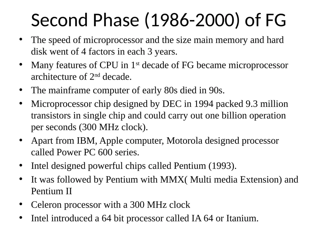
slide25. Second Phase (1986-2000) of FG The speed of microprocessor and the size main memory and hard disk went of 4 factors in each 3 years.
Many features of CPU in 1st decade of FG became microprocessor architecture of 2nd decade.
The mainframe computer of early 80s died in 90s.
Microprocessor chip designed by DEC in 1994 packed 9.3 million transistors in single chip and could carry out one billion operation per seconds (300 MHz clock).
Apart from IBM, Apple computer, Motorola designed processor called Power PC 600 series.
Intel designed powerful chips called Pentium (1993).
It was followed by Pentium with MMX( Multi media Extension) and Pentium II
Celeron processor with a 300 MHz clock
Intel introduced a 64 bit processor called IA 64 or Itanium.<br>
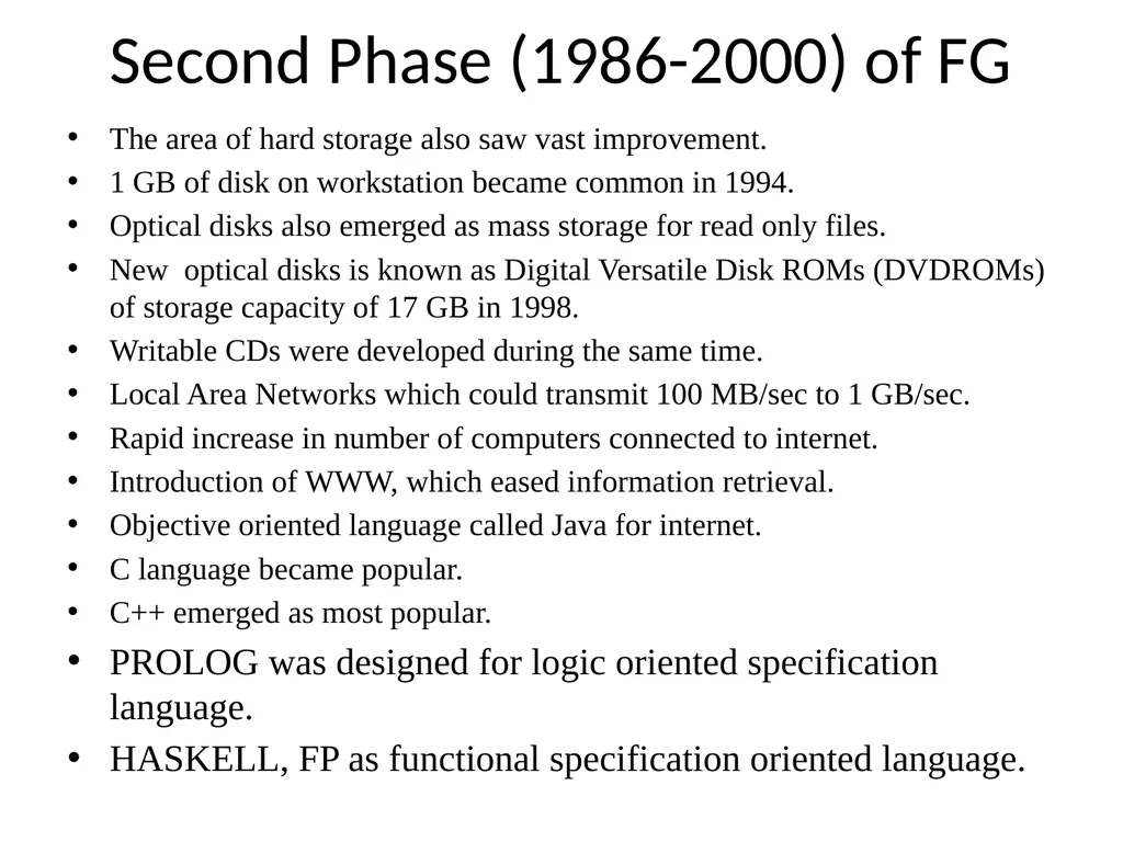
slide26. Second Phase (1986-2000) of FG The area of hard storage also saw vast improvement.
1 GB of disk on workstation became common in 1994.
Optical disks also emerged as mass storage for read only files.
New optical disks is known as Digital Versatile Disk ROMs (DVDROMs) of storage capacity of 17 GB in 1998.
Writable CDs were developed during the same time.
Local Area Networks which could transmit 100 MB/sec to 1 GB/sec.
Rapid increase in number of computers connected to internet.
Introduction of WWW, which eased information retrieval.
Objective oriented language called Java for internet.
C language became popular.
C++ emerged as most popular.
PROLOG was designed for logic oriented specification language.
HASKELL, FP as functional specification oriented language.<br>
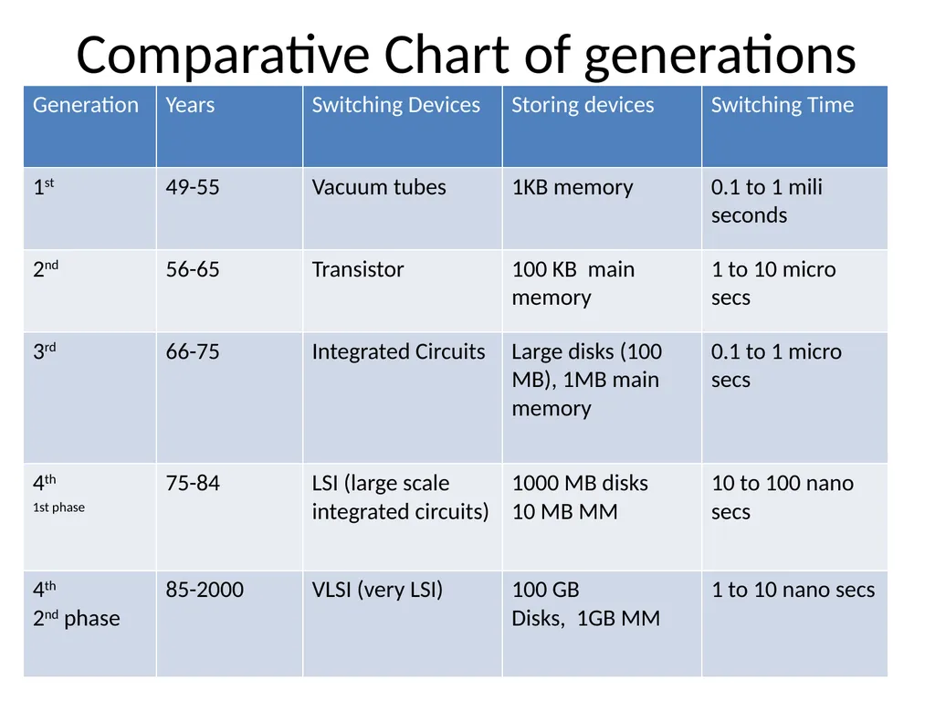
slide27. Comparative Chart of generations<br>
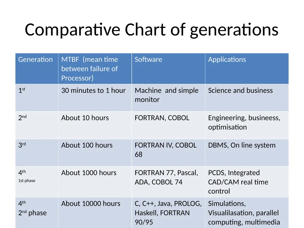
slide28. Comparative Chart of generations<br>
slide29. The 5th Generations FG is radically different from Von Neumann architecture.
Specification oriented programming and incorporate artificial intelligence features.
Changing the processor architecture. It is called Very large Instruction Word (VLIW). The size of one instruction is about 128 to 256 bits and has several parallel instructions.
Any time and any place access to data and processing. This is called as wireless enabled processor chips (Centrino of Intel), which are used laptop and hand held computers.
Demand for multimedia allowing users to use simple graphical user interface, listen to good quality audio, video on the desktop and mobile computers.
FG is wireless enabled multimedia and high performance mobile computers.<br>
slide30. 5th Generations ….. Fifth generation computing devices, based on
Artificial intelligence: Artificial Intelligence is the branch of computer science concerned with making computers behave like humans. The term was coined in 1956 by John McCarthy at the Massachusetts Institute of Technology. Artificial intelligence includes
Games Playing: programming computers to play games such as chess and checkers.
Expert Systems: programming computers to make decisions in real-life situations (for example, some expert systems help doctors diagnose diseases based on symptoms)
Natural Language: programming computers to understand natural human languages.<br>
slide31. 5th Generations …… Neural Networks: Systems that simulate intelligence by attempting to reproduce the types of physical connections that occur in animal brains
Robotics: programming computers to see and hear and react to other sensory stimuli
Voice recognition :Computer systems that can recognize spoken words. Comprehending human languages falls under a different field of computer science called natural language processing.
A number of voice recognition systems are available on the market. The most powerful can recognize thousands of words. However, they generally require an extended training session during which the computer system becomes accustomed to a particular voice and accent.
Such systems are said to be speaker dependent.<br>
slide32. 5th Generations …… Quantum computation : First proposed in the 1970s, quantum computing relies on quantum physics by taking advantage of certain quantum physics properties of atoms or nuclei that allow them to work together as quantum bits, or qubits, to be the computer's processor and memory. By interacting with each other while being isolated from the external environment, qubits can perform certain calculations exponentially faster than conventional computers. Qubits do not rely on the traditional binary nature of computing<br>
slide33. 5th Generations …… Molecular and nanotechnology: Nanotechnology is a field of science whose goal is to control individual atoms and molecules to create computer chips and other devices that are thousands of times smaller than current technologies permit. Current manufacturing processes use lithography to imprint circuits on semiconductor materials. While lithography has improved dramatically over the last two decades -- to the point where some manufacturing plants can produce circuits smaller than one micron(1,000 nanometers) -- it still deals with aggregates of millions of atoms. It is widely believed that lithography is quickly approaching its physical limits. To continue reducing the size of semiconductors, new technologies that juggle individual atoms will be necessary. This is the realm of nanotechnology.<br>
slide34. 5th Generations …… Natural language: natural language means a human language. For example, English, French, and Chinese are natural languages. Computer languages, such as FORTRAN and C,are not.
Probably the single most challenging problem in computer science is to develop computers that can understand natural languages. So far, the complete solution to this problem has proved elusive, although great deal of progress has been made. Fourth-generation languages are the programming languages closest to natural languages.<br>
slide35. 5th Generations …… Parallel processing and superconductors :
The use of parallel processing and superconductors is helping to make artificial intelligence a reality. Parallel processing is the simultaneous use of more than one CPU to execute a program. Ideally, parallel processing makes a program run faster because there are more engines (CPUs) running it. In practice, it is often difficult to divide a program in such a way that separate CPUs can execute different portions without interfering with each other.
Most computers have just one CPU, but some models have several. There are even computers with thousands of CPUs. With single-CPU computers, it is possible to perform parallel processing by connecting the computers in a network. However, this type of parallel processing requires very sophisticated software called distributed processing software.
Note that parallel processing differs from multitasking, in which a single CPU executes several programs at once.
Parallel processing is also called parallel computing.<br>
slide36. Moore’s Law 1965, Gordon E. Moore predicted that density of transistors in integrated circuits with double at regular interval of 2 years.
Since, 1965, his prediction became true.
Number of transistors per integrated circuit chip has approximately double in every 18 months.
In 1974, the largest Dynamic Random Access memory chip had 16 kbits, whereas in 1998 it has 256 mbits, as increase of 16000 times in just 24 years.
In 1984, the disks capacity in PCs was around 20 MB, where as it was 80 GB by 2004, which is 8000 fold increase.
Now it around 150 GB.
It has come without increase in price.
Moore’s law that foreseeable future will get more powerful computer with less price.<br>
slide37. Classification of computers Microcomputers
Mainframe
Supercomputers
But technology has changed and all computers use microprocessor as their CPU. Thus classification is possible only through their mode of use.
Palms
Laptop PCs
Desktop PCs
Workstations
Based on interconnected characteristics,
Distributed computers
Parallel computers<br>
slide38. Palm PCs/Simputer Which can be held in palm
High density packing of transistors on a chip
Palm with capabilities nearly that of PCs
It accept handwritten inputs using an electronic pen on a palm screen
Have small disk storage
Can be connected to wireless network
It has facilities to be used as mobile phone
Has the facility of fax and e-mail.
A version of MS OS called Window-CE is available for palm.<br>
slide39. Simputer Indian need for rural population called Simputer
Simputer is a mobile handheld computer with inputs through icons on touch sensitive overlay on the LCD display panel.
A unique feature of Simputer is the use of free open source OS called GNU/Linux.
Cost is low as there is no cost for software.
Another unique feature of Simputer is a smart card reader/writer which increases the functionality of the Simputer including possibility of personalisation of a single Simputer for several users.<br>
slide40. Laptop It is portable computer weighing around 2 kgs.
They have key board, flat screen liquid crystal display and pentium or power PC processor.
Colour display are also available
Normally WINDOWS OS is used.
LT come with hard disk (20 GB), CDROM and Floppy disk.
They are designed to conserve energy by using power efficient chips.
Trend of wireless connectivity to laptops so that they can read files from large stationery computers.
Lt are used for word processing and spreadsheet computing.<br>
slide41. Personal Computers (PCs) Most of the PCs are desktop machines.
Early PCs had intel 8088 microprocessor.
Intel Pentium IV is the most popular process.
The machines made by IBM are called IBM PCs.
IBM PCs mostly use MS-Windows, WINDOWS-XP or GNU/Linux as operating system.
Till 2004, PCs has 64 to 256 MB main memory, with 40 to 80 GB disk and now 160 GB
650 MB CDROM is also provided in PCs for multi-media use.
Apple Pc are called Apple Machintosh.
IBM Pcs are most popular.<br>
slide42. Workstations Woskstations are also desktop machines.
More powerful processors about 10 times that of PCs.
Most workstations have a large colour video display unit.
Normally they have main memory of around 256 MB to 4 GB and disk of 80 to 320 GB.
Workstations normally use RISC (Reduced Instruction Set Computer) processor such as MIPS (SIG), RIOS (IBM), SPARC (SUN), or PA-RISC (HP).
Some manufactures of workstations are silicon graphics (SIG), IBM, SUN Microsystems and HEWlett Packed (HP).
The standard OS of Workstations is UNIX and its derivatives such as AIX (IBM), Solaris (SUN), and HP-UX (HP).
Very good graphics facilities an large video screens are provided by most workstations.
A system called X Windows is provided by workstations to display the status of multiply process during their executions.
Most workstations have built in hardware to connect to a LAN.<br>
slide43. Servers Workstations are characterized by high performance processors with large screens for interactive programming,
While servers are used for specific purposes such as high performance numerical computing, web page hosting, data base store, printing etc.
Interactive large scale screen are not necessary.
Compute servers have high performance processors with large main memory, database servers have big on-line disk storage (100s of GB) and print servers support several high speed printers.<br>
slide44. Mainframe Computers Insurance, Banking and other companies need processor for large number of transactions on-line.
They require computers with very large disks to store several Tera bytes of data and transfer data form disk to main memory at several hundred Megabytes/sec.
The processing power needed from such computers is hundred million transactions per seconds.
These computers are much bigger and faster than workstations and several hundred times more expensive.
They provide extensive services such as user accounting, file security and control.
they are much more reliable
Few manufacturers, viz., IBM, and Hitachi.<br>
slide45. Supercomputers Super-computers are fastest computers available at any given time.
They are used to solve the problem which require intensive numerical computations.
Prediction of weather condition, designing supersonic aircrafts, design of drugs, modeling complex molecules.
All these problems require 1016 calculations.
These problems will be solved by 3 hours by a computer, which can carry a trillion calculations at a second.
These computers are called super-computers by 2004.
Super computers are built by interconnecting several high speed computers and programming them to work co-operatively to solve the problems.<br>
slide46. Supercomputers Conti……… They functions are expanded to analyze large commercial data base, produce animated movies and play games like chess.
Besides these functions, SC have large main memory of 16 GB and secondary memory of 1000 GB.
The speed of transfer of data from the secondary memory to main memory should be at least a tenth of the memory to CPU data Transfer speed.
All SC use parallelism to achieve their speed.<br>
slide47. Parallel Computers A set of computers connected together by a high speed communication network and programmed in such a way that they co-operate to solve a single large problems is called a Parallel computers.
Two types of Parallel computers:
Shared memory parallel computer (SMPC)
distributed memory parallel computer (DMPC)<br>
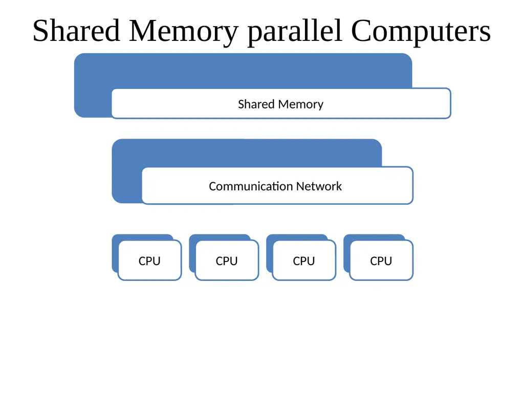
slide48. Shared Memory Parallel Computer Process of SMPC
A number of processing elements are connected to a common main memory by a communication network.
Programmes are written in such a way that multiple processor can work independently and co-operate to solve a problem.
Programming of such a computer is relatively easy provided the problem can be broken up into parts.<br>
slide49. Shared Memory parallel Computers<br>
slide50. SMPC Conti…… Limitations/Problems
It is not scalable beyond about 16 processors as all the processors share a common memory.
This memory is accessed via single communication network which gets saturated when many processors try to read or write from memory.<br>
slide51. DMPC A number of processors, each with its own memory are interconnected by a communication network.
A programme is divided into many parts and each computer works independently. Whenever computer need to exchange data to continue with computation they do so by sending messages to another via the communication net work.
Such computers are called message passing multi-computers.
DMPC scalable to over 1000 processors as each computers works reasonable independently and there are multiple communication paths to exchange messages.
A popular interconnection network is called hypercube.<br>
slide52. Other Types of Parallel Computers Ethernet System: the use of the shelf high standard performance PCs and interconnect them.
Ethernet speed of 1 Gbps is now available.
Linux system is available now.<br>
slide53. Reference Rajaraman, V. (2008), Fundamental of Computers, PHI Pvt. Ltl.
http://www.techiwarehouse.com/engine/a046ee08/Generations-of-Computer<br>
slide54. Input/Output Units Types of Input units, their advantage and disadvantages
Output units, their advantages and disadvantages<br>
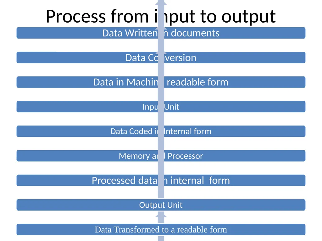
slide55. Process from input to output<br>
slide56. Description of Computer Input Units General Purposes: Keyboard and Desktop
Special purposes: Scanners, magnetic Ink character readers, Optical mark readers, Optical Character readers and bar code readers
Compact Disk Read Only Memory (CDROM): when large data are recoded for distribution of many users and for reading only and store it in computer memory.
650 MB of data can be recorded in CDROM.
Floppy disk is used if small amount of data is transferred such as 1.2 MB
Memory card or memory disk or flash memory: it is a solid state read only memory having 32 KB to 512 MB to store and distribute.
Storage device: Floppy, CDROM and Flash memory<br>
slide57. Keyboard It is used for manual entry of data
It is used for all types computers such as PC, Workstations, or notebook computer.
It is also called QWERTY keyboard as these are first six letters in the third row.
Categories of keys
Letter Keys -26 letters.
Digit Keys – 2 sets of digits keys.
Special Character Keys:- >< ?/{} [] (), “” \ | @ with the help of shift key.
Non- Printable Control Key. Back space, moving, cursor on above, insert space Bar.
Function Keys: F1,…… up to F15.
Functions of Non-tabulated keys: Backspace Key, Enter Key, Tab Key, Shift Key.<br>
slide58. Vodeo Terminal (VDU) What is VDU:
A video terminal or a video display unit consists of a televison screen and a keyboard.
When a key is pressed, the corresponding character is displayed on the screen.
Simultaneously, a cursor moves to the position where the next character will be displayed.
A cursor is small arrow, underline or a small rectangle which can be moved horizontally o vertically indicate the osition of character.<br>
slide59. VDU Conti…….. What is function of Cathod Rays
Cathode ray television tube is scanned by an electron bean to create a raster of horizontal lines. The intensity of the electron beam is increased at certain moments creating bright spots on the face of the tube. Each character is displayed by a matrix of 5 dots along horizontal direction and 7 dots in vertical direction.
A display normally has 80 characters per horizontal line and 24 such lines on the screen.
How typed Characters are displayed on the Screen
When key on the keyboard is pressed, the corresponding character is displayed on the screen because an appropriate coded series of electrical pulses are sent to computers memory.<br>
slide60. Output Units There are three principal devices to output
Printer: it is most common method
Video terminal
Computer output Micro-film: It is expensive and used in special cases.
Hard Copy Devices of Output: Printer and Microfilm as the data written using these devices can be read by human being.
Soft Copy Devices of Output: Floppy Disks, CDROM (R/W), Solid State Memory.
These are removable portable devices that the data in them can be read by another computer and stored in its memory for processing.<br>
slide61. Printers Two main categories:
Line Printers
Serial Character Printers
Line Printers: It prints complete line at a time. Printing speed varies from 150 lines to 2500 lines per minute with 96 to 160 characters on a 15 inch line.
Printer are available in almost all scripts: English, Arabic, cryillic (Russian), Hindi.
Two types of Line Printers: Drum printers and Chain printers<br>
slide62. Drum Printer Features of DP:
The character to be printed are embossed on its surface.
One complete set of characters is embossed for each print position on a line.
A printer with 132 character per line and a 96 character set will have on its surface 132 X 96 =12672 characters are embossed on it.
The codes of all characters to be printed on one line are transmitted from the memory of the to a storage units in the printer.
A set of print hammers, one for each character in a line are mounted in front of the drum. A character is printed by striking a hammer against the embossed character on the surface.
A carbon ribbon and paper are interposed between the hammer and the drum.
It is expensive and can not be changed quickly.<br>
slide63. Chain Printers Features of CP:
It has steel band on which character sets are embossed.
For a 64 character set printer, 4 sets of 64 characters each would be embossed on the band.
All the characters in the line are sent from the memory to the print buffer register.
Band is rotates with high speed.
When band rotate, a hummers is activated is activated when desire characters as specified in the buffer register comes in front of it.
For a 132 character per line, 132 hammers will be positioned to strike the carbon ribbon which is placed between the chain, paper and the hammer.
Different fonts and different scripts may be used in same printer.<br>
slide64. Serial printers Features of SP:
It prints one character at a time with the print head moving across a line.
It is normally slow and print 30 to 300 character per second.
The popular SP is called dot-matrix.
The print head consist of array of pins.
Characters to be printed are sent one character at a time from the memory to the printer. The character code is decoded by the printer electronics and activates the appropriate pins in the print head.
Many dot matrix are bidirectional: left to right and right to left.<br>
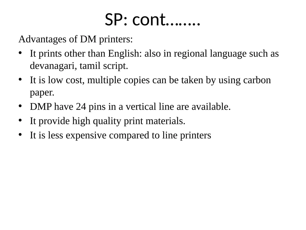
slide65. SP: cont…….. Advantages of DM printers:
It prints other than English: also in regional language such as devanagari, tamil script.
It is low cost, multiple copies can be taken by using carbon paper.
DMP have 24 pins in a vertical line are available.
It provide high quality print materials.
It is less expensive compared to line printers<br>
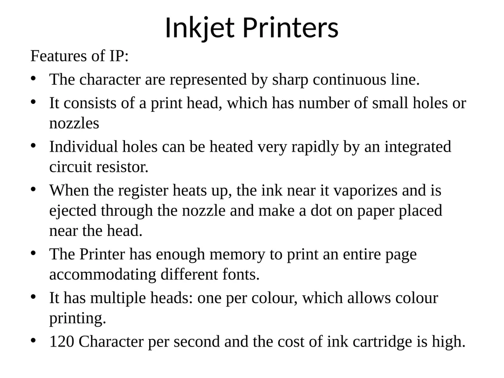
slide66. Inkjet Printers Features of IP:
The character are represented by sharp continuous line.
It consists of a print head, which has number of small holes or nozzles
Individual holes can be heated very rapidly by an integrated circuit resistor.
When the register heats up, the ink near it vaporizes and is ejected through the nozzle and make a dot on paper placed near the head.
The Printer has enough memory to print an entire page accommodating different fonts.
It has multiple heads: one per colour, which allows colour printing.
120 Character per second and the cost of ink cartridge is high.<br>
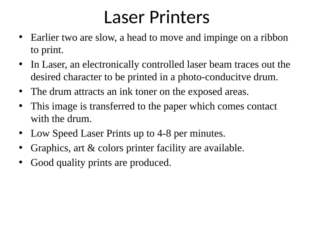
slide67. Laser Printers Earlier two are slow, a head to move and impinge on a ribbon to print.
In Laser, an electronically controlled laser beam traces out the desired character to be printed in a photo-conducitve drum.
The drum attracts an ink toner on the exposed areas.
This image is transferred to the paper which comes contact with the drum.
Low Speed Laser Prints up to 4-8 per minutes.
Graphics, art & colors printer facility are available.
Good quality prints are produced.<br>
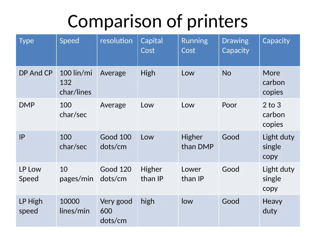
slide68. Comparison of printers<br>
slide69. Reference Rajaraman, V. (2008), Fundamental of Computers, PHI Pvt. Ltl<br>
slide70. Storage Unit Storage unit is ranked based on the following criteria
Access time
Storage capacity
Cost per bit of storage
Two types of Storage
Primary Storage Unit (Main Memory)
Secondary Storage Unit

Primary Storage Unit (Main Memory)
Faster Access time
Smaller storage capacity
Higher cost per bit of storage<br>
slide71. Storage Location and Address It is basis to all computers.
It is made up many small storage areas called locations or cells.
Each location can store fixed number of bits called word length.
Address of Location: it is used to identify the location.
Each location can hold either a data item or an instruction.<br>
slide72. Storage Capacity The capacity is defined in terms of bytes or words.
Storage capacity is commonly denoted as K (kilo), which is equal to 210 or 1024 bytes or characters.
32 kilo bytes means 32 X1024 = 32, 768 bytes or characters.
It is necessary to know word size in bits or bytes in order to determine the actual storage capacity of the computer.
It is necessary to know total number of bits per word or total words.
16 bit 4096 word memory is called 4096 location each with different address and each location storing 16 bits.
32 K16 – bits memory having 215 words with each word of 16 bits.
If word size of a memory is 8 bits (equal to a byte) then it becomes immaterial whether the memory capacity is expressed in terms of bytes or words.
Memory having 216 words with each word of 8 bits is simply reffered to 64 K memory.<br>
slide73. Why do need more BITS Meaning of 8 Bits, 16 bits and 32 bits computer: Word size in terms of total number of bits.
What is the advantage of having more number of bits per word instead of having more words of smaller size?
Example of High ways of 4 lanes, 8 lanes and 16 lanes
Greater bits means more rapid flow of electronic signal means faster computer.
What is Word Addressable Computer: fixed number of characters in each numbered address location. They apply fixed word length storage approach.
Character Addressable computer: the primary storage section is also designed in such a way that each numbered address can only store a single character. They employ variable word length storage approach.<br>
slide74. Merit and Demerit of Fixed and Variable Word Length Storage Approach FWLSA is normally used in large scientific computers for gaining speed of calculations.
Suppose in a FWLSA word length is eight characters, words are stored is less than five characters, then many storage will be unused.

VWLSA is used in small business computers for optimizing the use of storage space.
No problem of Unused space<br>
slide75. Types of Storage RAM: Random Access Memory
Primary storage is usually referred to as random access memory because it is possible to randomly selected
Use any location of this memory to directly store and retrieve data and instruction.
It is also referred to as read/ write memory because information.
ROM: Read Only Memory
Information is permanently stored.
The information can only be read and it is not possible to write fresh information into it.
When power is switched off, the does not wash off.<br>
slide76. Micro-programmes Special programmes are written to run the operations of low level of machine operations.
They are substitute of additional hardware
MP are written to aid the control unit in directing all the operations of the computer system.
ROMs are mainly used by computer manufactures for storing these micrprogramms, so that they can not modify the users.<br>
slide77. Programmable ROM It is possible for a user to customise a system by converting his own programms to micro-programs and storing them in PROM.
Once the users programmes are stored in PROM chip, they can usually be executed in a fraction of the time previously required.
Once the chip has been programmed, the recorded information cannot be changed, i.e., PROM becomes ROM.
PROM is non-volatile storage, i.e., the stored information remains intact even if power is switched off.<br>
slide78. Erasable PROM Another type of memory chip EPROM, that overcome this problem.
It is possible to erase information stored in an EPROM chip and chip can be reprogrammed to store new information using a special prom-programmer facility.
EPROM is erase by exposing the chip by ultraviolet light.
When an EPROM is in use, information can only be read and the information remains on the chip until it is erased.
EPROM are mainly used by R& D personnel because they frequently change the micro-programms to test the efficicny of the computer.<br>
slide79. CACHE MEMORY A special high speed memory is used to speed of processing by making current programs and data available to the CPU at a rapid rate.
The technique used to compensate the mismatching in operating speed between CPU and Main Memory is called cache memory.
It is a memory in hiding and is not addressable by the user of the computer system.
Cache memory makes main memory faster than it really is.
It improve the memory transfer rates and thus raising the processor speed.<br>
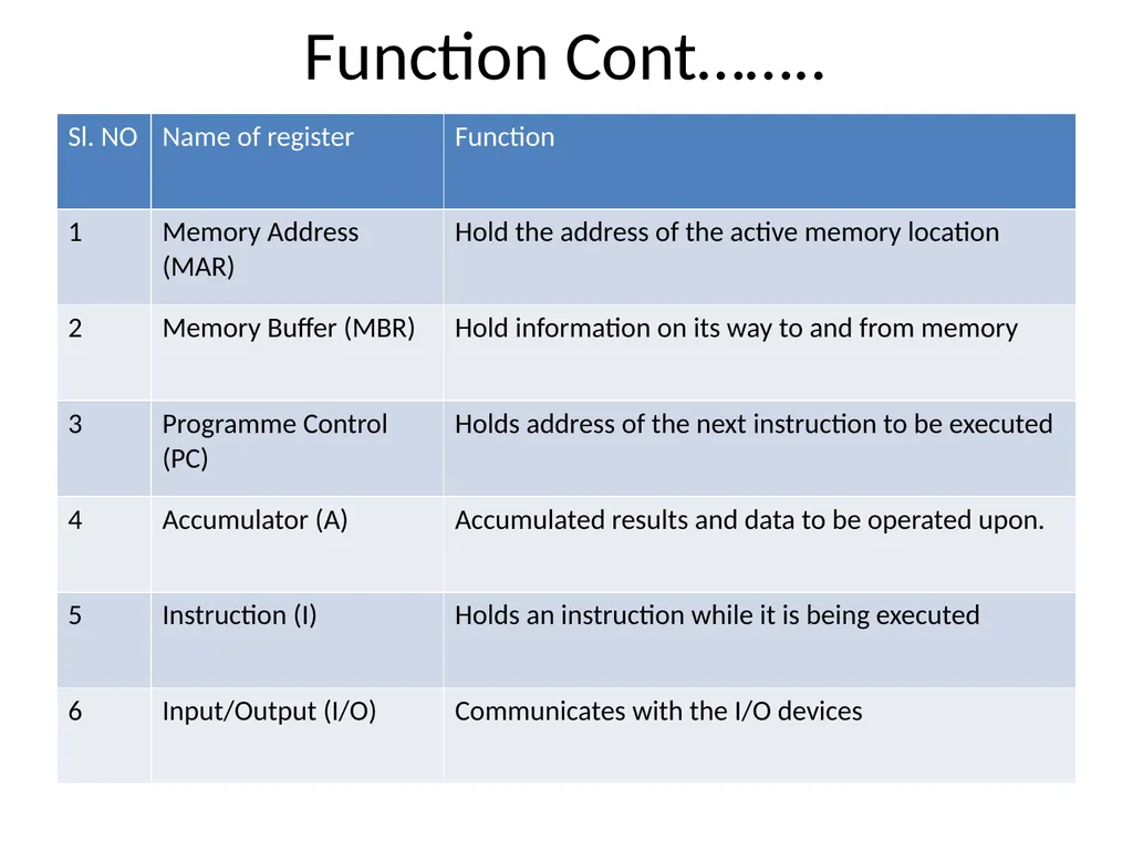
slide80. Registers Registers are special memory units which makes the moment of information between the various units satisfactory and makes speed up.

These are not considered as a part of the main memory and are used to retain information on a temporary basis.<br>
slide81. Function Cont……..<br>
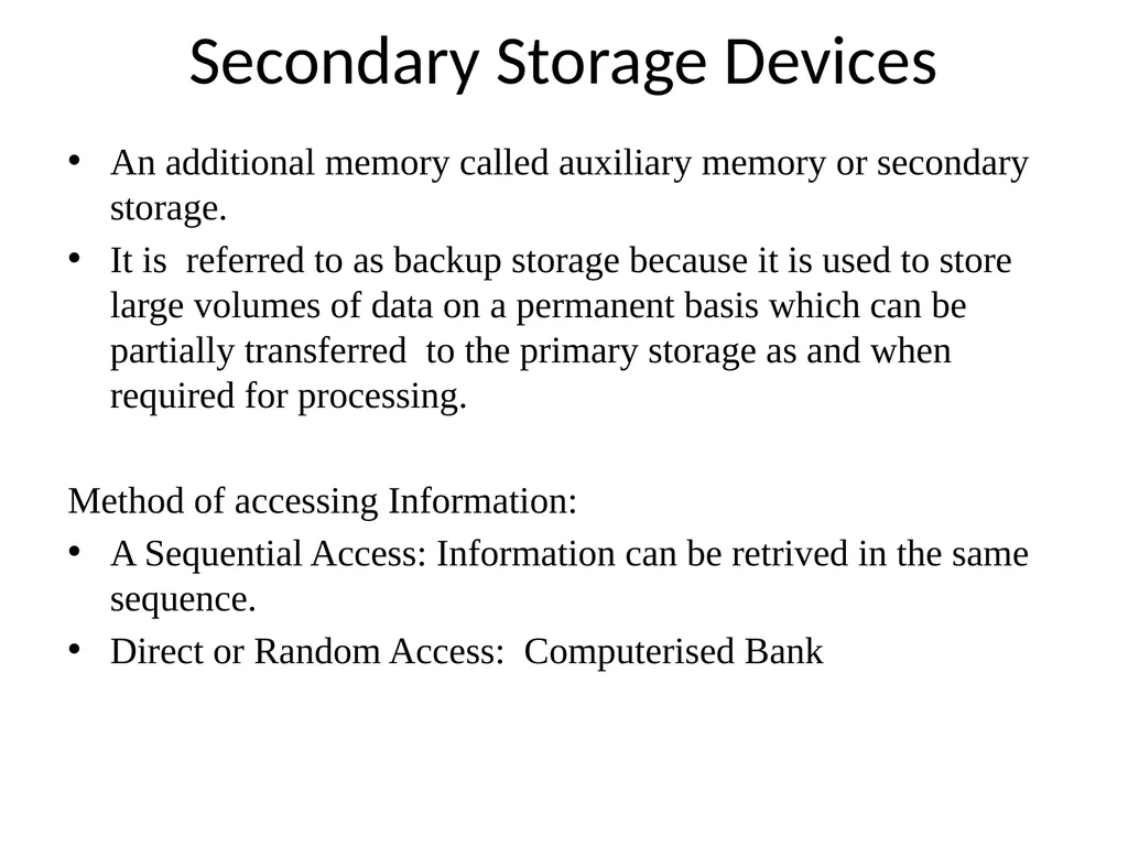
slide82. Secondary Storage Devices An additional memory called auxiliary memory or secondary storage.
It is referred to as backup storage because it is used to store large volumes of data on a permanent basis which can be partially transferred to the primary storage as and when required for processing.

Method of accessing Information:
A Sequential Access: Information can be retrived in the same sequence.
Direct or Random Access: Computerised Bank<br>
slide83. Reference Sinha, P.K. (1996), Computer Fundamental, BPB Publications, New delhi.<br>
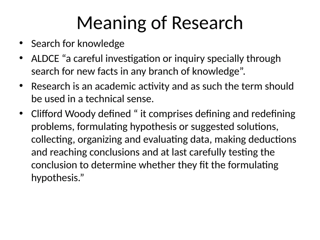
slide84. Meaning of Research Search for knowledge
ALDCE “a careful investigation or inquiry specially through search for new facts in any branch of knowledge”.
Research is an academic activity and as such the term should be used in a technical sense.
Clifford Woody defined “ it comprises defining and redefining problems, formulating hypothesis or suggested solutions, collecting, organizing and evaluating data, making deductions and reaching conclusions and at last carefully testing the conclusion to determine whether they fit the formulating hypothesis.”<br>
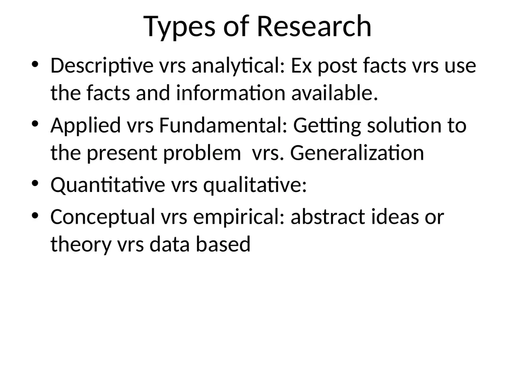
slide85. Types of Research Descriptive vrs analytical: Ex post facts vrs use the facts and information available.
Applied vrs Fundamental: Getting solution to the present problem vrs. Generalization
Quantitative vrs qualitative:
Conceptual vrs empirical: abstract ideas or theory vrs data based<br>
slide86. Sampling, Design and Size Sanatan Nayak
L-4
DE/SAS, BBAU<br>
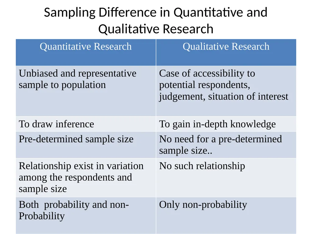
slide87. Sampling Difference in Quantitative and Qualitative Research<br>
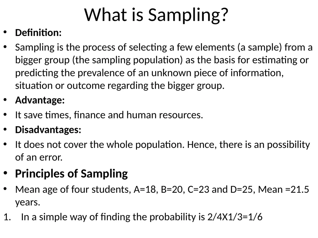
slide88. What is Sampling? Definition:
Sampling is the process of selecting a few elements (a sample) from a bigger group (the sampling population) as the basis for estimating or predicting the prevalence of an unknown piece of information, situation or outcome regarding the bigger group.
Advantage:
It save times, finance and human resources.
Disadvantages:
It does not cover the whole population. Hence, there is an possibility of an error.
Principles of Sampling
Mean age of four students, A=18, B=20, C=23 and D=25, Mean =21.5 years.
In a simple way of finding the probability is 2/4X1/3=1/6<br>
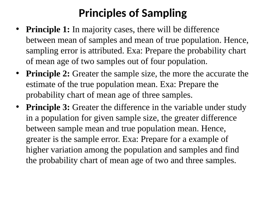
slide89. Principles of Sampling Principle 1: In majority cases, there will be difference between mean of samples and mean of true population. Hence, sampling error is attributed. Exa: Prepare the probability chart of mean age of two samples out of four population.
Principle 2: Greater the sample size, the more the accurate the estimate of the true population mean. Exa: Prepare the probability chart of mean age of three samples.
Principle 3: Greater the difference in the variable under study in a population for given sample size, the greater difference between sample mean and true population mean. Hence, greater is the sample error. Exa: Prepare for a example of higher variation among the population and samples and find the probability chart of mean age of two and three samples.<br>
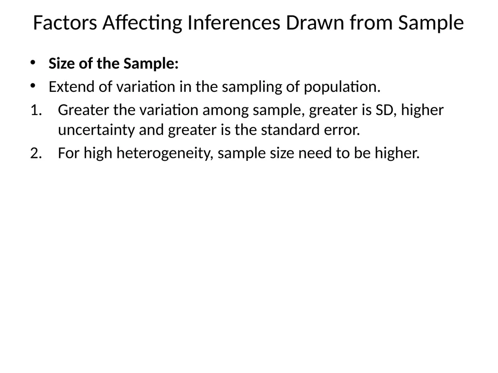
slide90. Factors Affecting Inferences Drawn from Sample Size of the Sample:
Extend of variation in the sampling of population.
Greater the variation among sample, greater is SD, higher uncertainty and greater is the standard error.
For high heterogeneity, sample size need to be higher.<br>
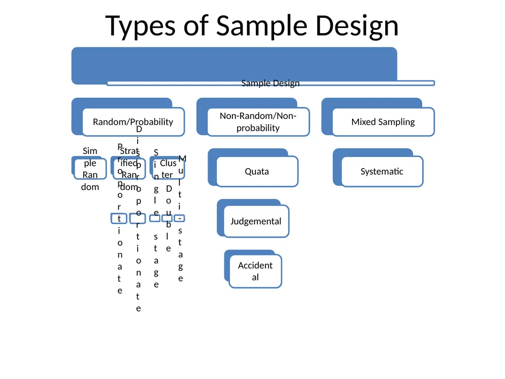
slide91. Types of Sample Design<br>
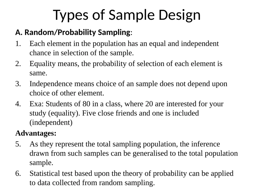
slide92. Types of Sample Design A. Random/Probability Sampling:
Each element in the population has an equal and independent chance in selection of the sample.
Equality means, the probability of selection of each element is same.
Independence means choice of an sample does not depend upon choice of other element.
Exa: Students of 80 in a class, where 20 are interested for your study (equality). Five close friends and one is included (independent)
Advantages:
As they represent the total sampling population, the inference drawn from such samples can be generalised to the total population sample.
Statistical test based upon the theory of probability can be applied to data collected from random sampling.<br>
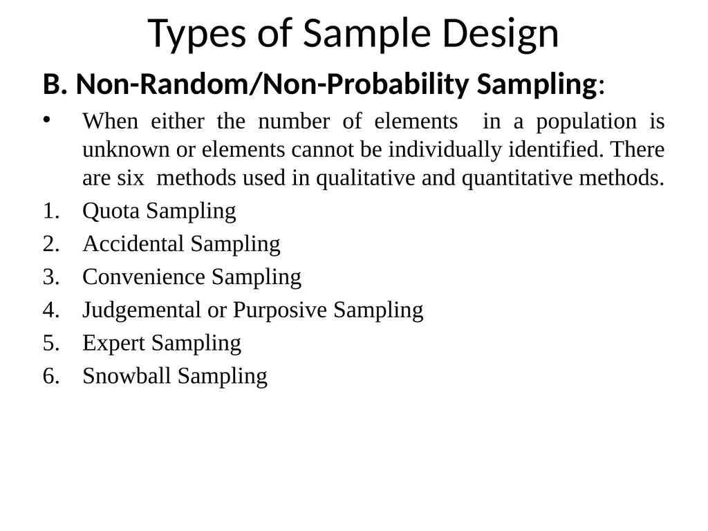
slide93. Types of Sample Design B. Non-Random/Non-Probability Sampling:
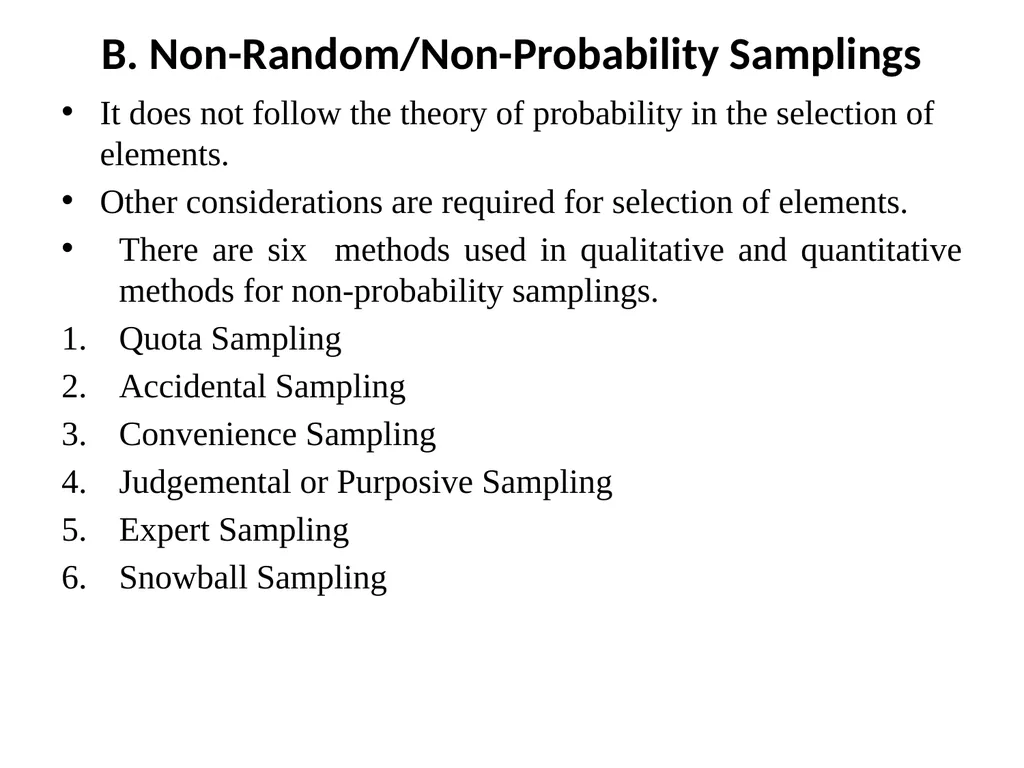
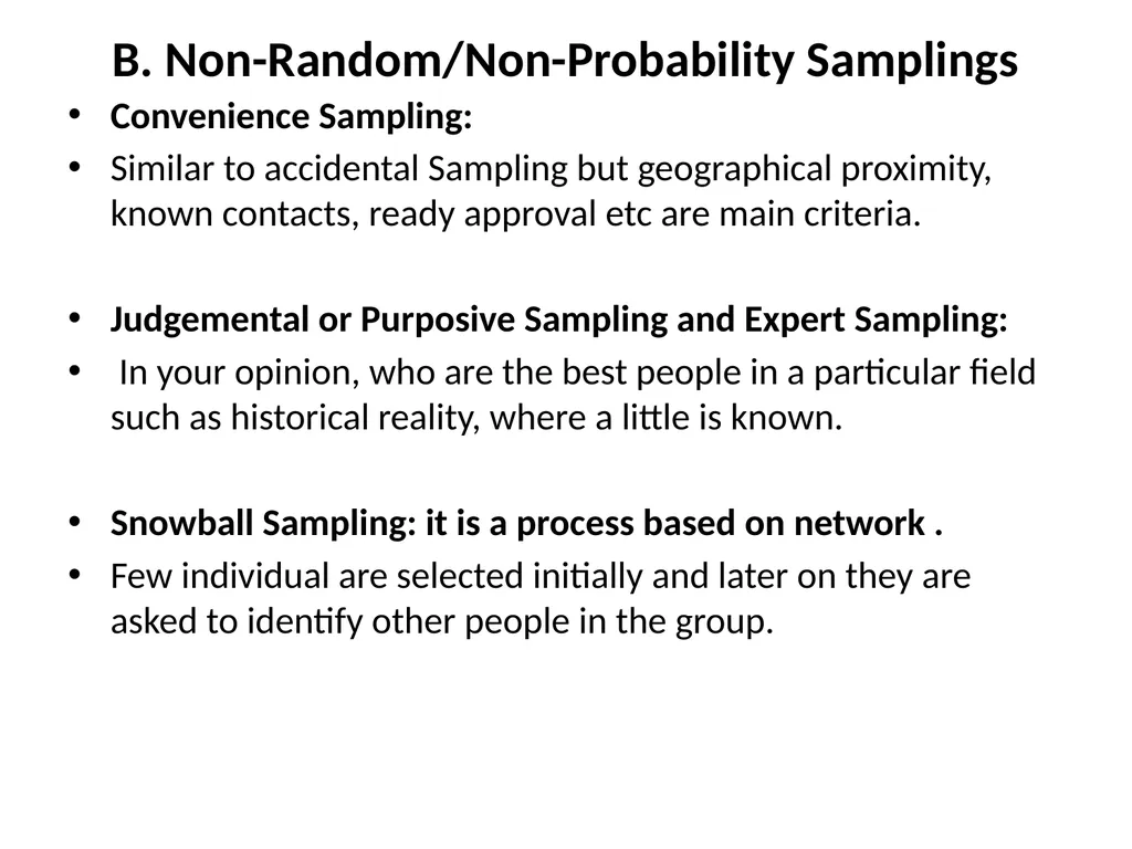
When either the number of elements in a population is unknown or elements cannot be individually identified. There are six methods used in qualitative and quantitative methods.
Quota Sampling
Accidental Sampling
Convenience Sampling
Judgemental or Purposive Sampling
Expert Sampling
Snowball Sampling<br>
slide94. Types of Sample Design C. Systematic /Mixed Sampling:
It has characteristics of both random and non-random methods.
Suppose 10% sample would be selected from 50 population. then, every 5th item would be selected from the population.<br>
slide95. Specific Random/Probability Sample Designs Simple Random Sampling
Stratified Sampling
Cluster Sampling
Sequential Sampling
Area Sampling
Multi Stage Sampling
Sampling with Probability Proportional to Size<br>
slide96. Specific Random/Probability Sample Designs Random/Probability Samplings:
The Fishbowl Draw:
Computer Programme:
Table of Randomly generated Numbers:
No of Samples= N(N-1)....(N-n+1)/n!
Probability of getting a sample =n!/N(N-1)....(N-n+1)<br>
slide97. A. Specific Random/Probability Sample Designs Stratified Random Sampling:
To reduce the variability or heterogeneity in the large sample population is the objective.
If population is not homogenous group, then SST is normally applied.
The population is divided in to many sub-population, which is called strata. Population within stratum is homogeneous, but across stratum, it is heterogeneous.
SST is more reliable and provides detailed information.
Important Questions on Stratified Sampling Techniques:
How to form a strata?
How should items be selected from each stratum?
How to allocate the sample size of each stratum?<br>
slide98. A. Specific Random/Probability Sample Designs How to form a strata?
The elements within strata must be homogeneous.
It is done based on experience of the researcher.
Pilot study needs to be done carefully.
How should items be selected from each stratum?
Either random sampling method or systematic sampling will be applied.
How many sample or How to allocate the sample size of each stratum?
Proportional sampling method.
Exa: Total population= 8000, population of three stratum, P1=4000, P2=2400, P3=1600, total sample size, n=40,
Pi= proportion of population in each stratum, then how to calculate sample size in each stratum?<br>
slide99. A. Specific Random/Probability Sample Designs How many sample or How to allocate the sample size of each stratum?
Then, how to handle when comparison is made across stratum along with variability in size and elements?
Then, disproportionate sampling design is required. Proportionately larger sample in larger strata and smaller sample in smaller strata.
Write the Formula:
This method is called optimum allocation of samples through disproportionate sampling.
Example:
Then how to optimise cost?<br>
slide100. A. Specific Random/Probability Sample Designs Cluster Sampling:
In case of large population of one city or a country CS is taken.
Conveniently and randomly take a smaller area of one bigger area, i.e., cluster.
Clusters are visible or easily identifiable small group in a geographical proximity or common characteristics.
Sampling from each cluster can be done through SRS or systematic sampling.
Exa: Problems of higher education in the country.
Clustering sampling is extremely useful for random sampling.<br>
slide101. A. Specific Random/Probability Sample Designs Different Stages of Cluster Sampling:
CS may be start from country or territory level. Then choose similar state based on socio-economic profile or all states.
Then, select one or more educational institutions of higher education.
Then, one or more academic programme from each institution may be selected.
Students of a particular academic year to be taken.
Proportionate basis students may be identified.<br>
slide102. A. Specific Random/Probability Sample Designs Area Sampling:
If cluster happens to be an geographical area, then CS known as AS.<br>
slide103. A. Specific Random/Probability Sample Designs Multi Stage Sampling:
It is based on the principle of cluster sampling.
Bank Efficiency in India.
First, select a state, then select many districts. Then chose all banks in the chosen districts. Two stage sampling.
Then add certain towns, and interview all banks. Three stage sampling.
If banks are selected on sample basis from selected towns, then four stage.
If random is on all stages, that is called multi stage random sampling method.<br>
slide104. A. Specific Random/Probability Sample Designs Sampling with Probability Proportional to Size:
If cluster sampling units do not have the same number, then random selection process, where probability of each cluster being included in sample.
The actual cluster selected in this way do not refer to individual elements but it indicates which cluster and how many are selected from each cluster.
Exa. There are 15 cities and cluster of stores in each city. Select 10 stores from the 15 cities.<br>
slide105. A. Sampling with Probability Proportional to Size<br>
slide106. A. Specific Random/Probability Sample Designs Sequential Sampling
It is complex in nature. Ultimate sample is not fixed and depend the information yielded as survey progress.
If a particular lot is selected or rejected based on single sample, it is called single sample.
If decision is taken on the basis of two samples, it is called double sample.
If decision is taken on the basis of many samples but sample size is certain and known in advance, it is called multiple sampling.
If decision is taken on the basis of many samples but sample size is not certain and not known in advance, it is called sequential sampling.<br>
slide107. B. Non-Random/Non-Probability Samplings It does not follow the theory of probability in the selection of elements.
Other considerations are required for selection of elements.
There are six methods used in qualitative and quantitative methods for non-probability samplings.
Quota Sampling
Accidental Sampling
Convenience Sampling
Judgemental or Purposive Sampling
Expert Sampling
Snowball Sampling<br>
slide108. B. Non-Random/Non-Probability Samplings 1. Quota Sampling:
Based on easy access and convenience on visible characteristics such as gender, race, caste etc.
Process will continue till you have easy access to required number of respondents.
Advantages:
Least expensive and no sampling frame.
Disadvantages:
No probability sampling and can not be generalised.
2. Accidental Sampling
Similar to Quota sampling but not based visible characteristics.
Stop collecting data when required number are done.
It is mostly applied in the area of market research and newspaper reports.<br>
slide109. B. Non-Random/Non-Probability Samplings Convenience Sampling:
Similar to accidental Sampling but geographical proximity, known contacts, ready approval etc are main criteria.

Judgemental or Purposive Sampling and Expert Sampling:
In your opinion, who are the best people in a particular field such as historical reality, where a little is known.

Snowball Sampling: it is a process based on network .
Few individual are selected initially and later on they are asked to identify other people in the group.<br>
slide110. C. Systematic/Mixed Sampling It has both random and non-random characteristics.
Sampling frame is designed into number of segments called intervals.
From the first interval, first element is selected on random basis.
Width of interval (k)=Total population (N)/sample size (n)
Sampling frame is needed.<br>
slide111. Calculation of Sample Size Quantitative Research:
It depend on the purpose of the findings in quantitative research.
Greater the heterogeneity, greater the sample size.
Level of confidence or test of hypothesis.
Degree of accuracy
Level of variation (SD).

Qualitative Research:
Sample size is less important in qualitative research.
Sampling design may be on purposive, judgemental, expert, accidental and snowball method.<br>
slide112. Bias and Error Difference between sample mean and population mean is called error.
It caused due to sampling selection.
There are large number of errors as there are many alternative samples.
Therefore, there is possibility to have one summary of measure of sample error, which is called as Mean Square Error (MSE).
However, bias and error can take place at data collection, data entry and analysis. These errors are called Non-Sampling Errors. These errors are taken place in sampling as well as Census.
There is difference between error and bias, however both affect MSE.<br>
slide113. Bias and Error First part of equation 1.4 is termed bias.
First theory of sample is equal probability of selection method (EPSEM).
Second principles is known as sampling variance of mean. Its square root as the standard error of the mean.
MSE (y)=B2 +sampling variance of mean
Exa 1 and 2: See in excel the Daily wage of Six Employees.<br>
slide114. References Kumar, Ranjit (2014), Research Methodology: A Step by Step Guide for the Beginners, Sage Publication, New Delhi.

Roy, Taru Kumar et al., (2016), Statistical Survey Design and Evaluating Impact, Cambridge University Press, New Delhi.

Ladu Singh L. (2018), Survey Sampling Methods, Eastern Economy Edition, New Delhi.

Bryman, Alan (2009), Social Research Methods, OUP, New Delhi.
Kothari, C.R. (2004), Research methodology, New age International Publications, New Delhi.<br>
slide115. Methods of Research Research Process
Formulating Research Problems
Extensive Literature Survey
Development of Hypothesis
Preparing Research Design
Determining Sample Design
Data Collection
Execution of Project
Analysis of Data
Hypothesis testing
Generalization and Interpretations
Preparation of Reports<br>
slide116. Data: Sources and Methods The term data (singular datum) refers to facts from which other facts may be deduced.
Bertrand Russel remarks “the questions of Data has been mistakenly, as I think, mixed up with the questions of certainty. The essential characteristics of a datum is that it is not inferred.”
Difference between Facts and Data
A fact is statement of actuality. It involves tangible things as well as sentiments and feeling in social studies.
A datum is fact on which reasoning is based and thus serves as base for analyzing and interpretations.<br>
slide117. Sources of Data<br>
slide118. Methods of Collecting Data Observation Method
Interview Method
Questionnaire method
Schedule
Other Methods
Warrant cards
Distributors Audits
Pantry Audits
Consumer Panels
Using mechanical device
Projective Techniques
Depth Interviews
Contents Analysis<br>
slide119. Observation Methods Behavioral sciences
Investigators own direct observation without asking any questions to respondents
It deals with current happening not with past behaviour
It is independent of respondents behavior
Limitations
Expensive
information provided in this method is limited
Unforeseen factors also affect the methods<br>
slide120. Experimental Methods It is applied with a good deal of success in certain cases to measure a group of factors which operate as a social programme.
Example: Impact of modern technology on the behavior of farmers (with and without situations).
Teaching on certain issues: With exhibition and without it. With television and without it.
The methodology of an experimental in nature has not penetrated far into the social sciences.<br>
slide121. Survey methods It is widely used technique.
Economic Survey was first introduced in UK.
Prof. G.F. Warren experimented his systematic study which is published in 1911.
Survey defined by Campbell and Katona as “Many research problems require the systematic collection of data from populations or samples of population through the use of personal interviews or other data gathering devices. The study are usually called surveys, especially when they are concerned with large or widely dispersed groups of people. When deal with only a fraction of a total population, a fraction representation of the total, they are called sample surveys”.<br>
slide122. Characteristics of Survey Methods It gets response directly from respondents
It is representative sample of population.
It provides maximum information for a given amount of effort, time and expenditure.
It is conducted in natural environment
Types of Survey
Complete Enumeration: study of all individual in the universe
Case studies: Intensive investigation and analysis of individuals or families<br>
slide123. Characteristics of Case study Definitions: it is intensive study of all details of the domestic life of few carefully chosen families. To work it well requires a rare combination of judgment in selecting cases and or insights and sympathy in interpreting them.
According to Palmer, a case study characterize,
Which are common to every individual
Variation of these commons attribute the characteristics of groups
Other characteristics which belong uniquely to the individuals<br>
slide124. Sample Survey It is the study of the sample of whole population which provides information which could be generalized by use of adequate sampling criteria and with the aid of statistical methods.
Types of Sample Surveys:
Non-Controlled: it is employed as an exploratory technique.
Controlled: Standardization of Observational methods
Formulated hypothesis
Prepare questionnaire
Select a sample to be studied.
Seeks formal answers to the questions<br>
slide125. Survey Procedures Framing a questionnaires
A set of questions to be answered by the informant without the personal aid of an investigator or enumerator.
Advantage of mailed questionnaires:-
Economical
Convenient
Standardized words
Drawbacks:-
Not sure about our sample of information
Adequate replies.
Schedules:
A Schedules is a data recording devices where the interviewer fills up the form.<br>
slide126. Difference between Questionnaires and Schedule<br>
slide127. Collection of Data Through Questionnaire Main Aspects of Questionnaire
General form: Structured or Unstructured
Closed or open ended
Measurement vrs. Categorical questions<br>
slide128. Interview Methods Personal Interview: Face to Face contact
Structured interview: predetermined questions and standardized techniques of recording
Unstructured interview: not a systematic predetermined questions.
Focused interview: based on respondents experience and its effects
Clinical Interview: feeling or motivation or with the course of individuals life experience
Non-Directive interview: No Direction from the interviewer<br>
slide129. Collection of Secondary Data Published data of various publications of central, state, and local governments
International bodies, UNO, UNDP, ILO, IMF, and other national Govts.
Technical and trade journals
Books, magazines and newspapers
Reports and publications of various associations connected with business, industry, banks, stocks exchange.
Reports prepared by scholars, researchers, universities, institutes.
Public records and statistics, historical documents and other sources of published information.
Internet, E-journals, E-database<br>
slide130. Characteristics of Secondary data Reliability of data: who, when, what sources, was proper method applied, any bias of the compiler, what level of accuracy.
Suitability of Data: one enquiry may not be good for another enquiry.
Adequacy of Data: level of accuracy is inadequate, then researcher should not be used.
Selection of Appropriate Methods
Following factors must be kept in mind
Nature, scope and objective of enquiry
Availability of funds
Time factors
Precision required<br>
slide131. Reference Kothari, C.R. (2004), Research methodology, New age International Publications, New Delhi.
Bryman, Alan (2009), Social Reserch Methods, OUP, New Delhi.
Kumar, Ranjit (2014), Research Methodology: A Step by Step Guide for the Begginers, Sage Publication, New Delhi.<br>
slide132. Introduction to Stata<br>
slide133. What Shall We Cover Introduction to Stata
Data Entry, File creation, saving and reopen
Data Processing:
Data Validation for both categorical and Measurement data
Data Manipulation
Data Tabulation
Data Interpretations
Data Analysis
1. Descriptive Statistics (three commands)
2. Modelling of Time series (Regression, Panel Regressions) and Cross Section analysis (Dummy, Logit and Probit analysis)

Use of large scale data such as NSS, Census and NFHS

Examination Pattern: MT-II, MT-III (Term Paper), End-Semester Examination.<br>
slide134. Introduction It is a multi-purpose statistical package to help you explore, summarize and analyze datasets.
A dataset is a collection of several pieces of information called variables (usually arranged by columns). A variable can have one or several values (information for one or several cases).
Statistic package developed by Stata Corporation
Forms of Stata
Stata Intercooled (IC)
Small
Extended (Special edition)
Types of Windows
Command/ Review window, Variable Window, Output window, Data editor/browser window, Do File Editor<br>
slide135. Comparison of Stata<br>
slide136. Manuals of Stata Manual of Stata (16 volumes)
Stata Getting Started: Operating System
Stata Users Guide: Command more General
Stata base References Manuals (four Volumes): details on command and help files
Stata Graphic Manual Reference (Specialized manuals)
Stata Programming Reference manuals<br>
slide137. Reading Materials Hamilton (2004)
Kohler and Kreuter (2004)
Hills and De Stavola (2002)
Saphia Rabe-Hesketh, Brain Everitt (2003), A Handbook of statistical Analysis Using Stata, Chaman and Hall/CRC
Lang and Frees (2003), Regression Model Categorical dependent Variable using Stata
Clevel, Gould and Gutiereerd (2004): An Introduction to survival Analysis Using Stata
Hardin and Hilbe (2001), Generalised Linear Model and Extension
www. Stata.com/bookstore/statabooks.html
Through Internet: FAQ
Concept wise:
Oscar Torres-Reyna, Data Consultant, otorres@princeton.edu<br>
slide138. How to write Syntax Put help language
[by varlist:] command [varlist] [=exp] [if] [in] [weight] [using filename] [, options]
[by varlist:] instruct the stata to repeat the command for each combination of values in the list of variables varlist
Command is the name of the command
Varlist is the list of variables
=exp is the expression
[If exp] restrict the command to the subset of the observation that satisfies a logical exp
[In range] restrict the command to those observations whose indices lie in a particular range
[weight] allows weight to be associated with observation
[using] specify the filename to be used
[,options] is only needed if options are used<br>
slide139. Stata Commands For loading (or importing) and saving in main memory: use, infile, insheet, infix, save, outfile, outsheet
Data Manipulation: generate, egen, edit, sort, recode, xtile, pctile
Tabulation: tab, summarize, table, tabstat
Combining data into two files: append, merge, mmerge, xmerge
Command on reshaping: reshape, compress, collapse, separate
For controlling working environment of Stata: log, cmdlog, more, for, cd dir, type, shell, mkdir, copy, erase, help, search, view
Auxiliary information: label, notes, rename
Displaying status of data: describe, inspect, cf, compare, browse, list, count<br>
slide140. 1. Data Entry and Creation of Files Three types of files are in stata:
Data File (.dta)
Command file (.do)
Output file (.log)
How to Create a Data File
How to enter the data
Rename the variables
Label the variables (See help menu)
Label define the variables
Label value the variables
Save the file
Locate the file in the disk D/E/F drives.<br>
slide141. Command and Output File How to open a command/do file
Cmdlog using table1.do
How to close a command file
Cmdlog c
How to open a output file
Log using table1.log
How to close a output file
Log c<br>
slide142. Knowing about the data File Use of basic Commands
Describe, List, Codebook, label list, di _N, browse for the file
Summarize for the measurement variables
Tab and histogram for categorical variables
Use of other graphs like bar dot, histo, pie and box

Open the existing do.file
Cmdlog using table1.do, append
save the existing file

Open the existing output file
Log using table1.log, append
Open the existing dta.file

Open the existing Data file
Use table1
Shifting to another data file
Use table2, clear<br>
slide143. 2. Data Processing in Stata Data validation: summarize for measurement variables, tab for categorical variables.
Data manipulation: generate, merge, reshape, egen, append, by, collapse, xtile, sort, recode, pctile.
Data Tabulation: Tab, table and tabstat
Data Interpretation: descriptive vrs models.<br>
slide144. 2.1.Data Validation 1. Validation of Data: Check points, Data coding, Convert open end to close end, Types of variables
a. Categorical variable
b. Measurement Variable<br>
slide145. 2.2. Data Manipulation 1. Generation of New Variables
Generating a variable
Gen pcl=land/fsize
Grouping of Measurement Data
Grouping with Cut Points
Gen sizegr=recode(size, 5,7,12)
Label define sizegr 5 “small” 7 “medium” 12 “large”
2. Equal width
Gen sizegrl = autocode(fsize, 3, 0,9)
3. Equal frequency
Xtile sizegr = size, nq(4)<br>
slide146. 2.2. Data Manipulation To understand more on nature of Households
Create a new file as table2
Create gender, edu, age, occupation

2. Use of merge command
Master file vrs. Working file
Use table1
Sort hhno
Save, replace
Use table2, clear
Sort hhno
Merge hhno using table1, keep(caste religion fsize land)
Save, replace<br>
slide147. 2.2. Data Manipulation 3. Use of Collapse Command
In the table2, collapse fsize and income
Save in temp.files and take to table1.
Merge it in table1
Then use collapse
Collapse (sum) income, by (hhno)
Collapse (count) fsize, by (hhno)
4. Use of egen Command
Within the table2, we can collapse some of the variables by using egen command
egen new var= event(var), by (aspect)
egen totalincome= sum(income), by (hhno)
Then, use table command for understanding the relationship between categorical and measurement variable.
duplicates drop hhno, force<br>
slide148. 2.2. Data Manipulation 5. Use of by Command
sort educationby education: tab caste gender, row
by occupation: tab caste religion
6. Use of xtile Command
xtile agegr = age, nq(5)<br>
slide149. 2.3. Data Tabulation 1. Frequency Distribution between Categorical with Categorical Variable
tab caste religion
tab caste religion, row col
Test of Association
tab caste religion, row col chi2

2. Descriptive Statistics between Categorical with Measurement variable(s)
table caste, c(mean land sd land min land max land) row f(%5.2f)

3. Descriptive Statistics among Measurement variable(s)
tabstat land age income, s(mean sd min max) f(%5.2f)<br>
slide150. 2.3. Data Tabulation 4. tab and table
Use of by
by gender: summarize income
by income: tab gender
by income, sort: tab gender
by gender income, sort: summarize age
By caste: table edu gender, c(mean age) f(%5.2f)<br>
slide151. Use of Large Scale data Introduction to NSS Data
Introduction to NSS Data 69th Round
How 69th Round Data is different from small data
How to feel the Data (Describe, List, Codebook, label list, di _N, browse for the file)
Use of few more command (if, in, weight, recode, xtile, regress, factor)
Descriptive Statistics
Inequality Analysis
Regression Analysis: Multiple regression, Dummy and Logit regression
Factor Analysis or Indexing<br>
slide152. Inequality Measurement on Consumption Expenditure xtile mpce_qt_r= mpce [w=weight] if sector==1, nq(5)
xtile mpce_qt_u=mpce [w=weight] if sector==2, nq(5)
gen mpce_qt2=mpce_qt_r if sector==1
replace mpce_qt2=mpce_qt_u if sector==2
drop mpce_qt_r mpce_qt_u
tab mpce_qt2<br>
slide153. Component of The Term Paper Based on the survey data, fin out the following.
Descriptive statistics
Inequality Measurement: Deciles, Quintiles
Regression Analysis: Multiple Regression, Dummy (Anova and Ancova)
Logit Regression: Poverty line estimation and analysis
Multi Dimensional Poverty estimation
Indexing: Factor Analysis<br>
slide154. Regression Analysis Time Series Analysis
Multiple Regession:
regress pcexp expdur expnondur expservice
Double log model
Gen lpcexp=log(pcexp)
regress lpcexp lexpdur lexpnondur lexpservice
Log-lin Model
Regress lpcexp year
Use keep command
lin-log model
Regress pcexp lexpdur

Structural change model<br>
slide155. Regression Analysis Regression Analaysis
regress mpce hhnntotal [w=weight]
regress mpce hhnntotal [w=weight] if state==9
regress mpce hhnntotal [w=weight] if district==927
regress mpce hhnntotal [w=weight] if district==927 & sector==2

regress mpce hhnntotal new_edu_male [w=weight]
regress mpce hhnntotal new_edu_male [w=weight] if state==9
regress mpce hhnntotal new_edu_male [w=weight] if district==927
regress mpce hhnntotal new_edu_male [w=weight] if district==927 & sector==2

regress mpce hhnntotal new_edu_male new_edu_female [w=weight]
regress mpce hhnntotal new_edu_male new_edu_female [w=weight] if state==9
regress mpce hhnntotal new_edu_male new_edu_female [w=weight] if district==927
regress mpce hhnntotal new_edu_male new_edu_female [w=weight] if district==927 & sector==2<br>
slide156. Regression Analysis recode landpossessed 1=0.005 2=0.02 3=0.21 4=0.41 5=1.01 6=2.01 7=3.01 8=4.01 10=6.01 11=8.01 12= 10, gen(new_land)
summa new_land

regress mpce hhnntotal new_edu_male new_edu_female new_land [w=weight]
regress mpce hhnntotal new_edu_male new_edu_female new_land [w=weight] if state==9
regress mpce hhnntotal new_edu_male new_edu_female new_land [w=weight] if district==927
regress mpce hhnntotal new_edu_male new_edu_female new_land [w=weight] if district==927& sector==2<br>
slide157. Post-Mortem (Multi-colinearity, Hetero-scadasticity, Auto-correlation) Hetero-scadasticity
hettest
imtest
hettest mpce (variable wise)

Multi-colinearity
corr mpce hhnntotal new_edu_male new_edu_female new_land [w=weight]

Auto-correlation
vif (variance influential factor)<br>
slide158. Dummy Regression Anova Model:
Create a dummy variable, by using
Does gender play any discriminatory role ?
Tab gender, gen(gender)
Table gender, c(mean mpce, sd mpce min mpce max mpce)
regress mpce gender1 [w=weight]
regress mpce gender1 [w=weight] if state==9
regress mpce gender1 [w=weight] if district==927
regress mpce gender1 [w=weight] if district==927 & sector==2
regress mpce gender1 [w=weight] if district==927 & sector==1
Does Caste plays any discriminatory role ?
Tab caste, gen(caste)
Table caste, c(mean mpce, sd mpce min mpce max mpce)<br>
slide159. Dummy Regression Ancova M
How gender and family size impact on the MPCE?
regress mpce gender1 hhnototal [w=weight]
regress mpce gender1 hhnototal [w=weight] if state==9
regress mpce gender1 hhnototal [w=weight] if district==927
regress mpce gender1 hhnototal [w=weight] if district==927 & sector==2
regress mpce gender1 hhnototal [w=weight] if district==927 & sector==1
How Caste and Family Size impact on the MPCE?
Tab caste, gen(caste)
regress mpce caste1 caste2 caste3 hhnototal [w=weight]<br>
slide160. How to estimate poverty line See Rangarajan Commitee Report, p.4
Rs.972 for rural areas and Rs.1407 for urban areas
recode mpce (0/972=1) (972.01/174286=2) if sector==1 , gen (pov_r)
recode pov_r (. = 0)
recode mpce (0/1407=1) (1407.01/174286=2) if sector==2 , gen (pov_u)
recode pov_u (. = 0)
gen pov_i= pov_r + pov_u
label var mpce "Monthly Per Capita Expenditure"
label var pov_r "Poverty in Rural Sector"
label var pov_u "Poverty in Urban Sector"
label var pov_i "Poverty in Both Sector"
label define pov_r 1 "Below Poverty Line" 2 "Above Poverty Line"
label values pov_r pov_r
label define pov_u 1 "Below Poverty Line" 2 "Above Poverty Line"
label values pov_u pov_u
label define pov_i 1 "Below Poverty Line" 2 "Above Poverty Line"
label values pov_i pov_i<br>
slide161. How to Estimate Logit Model Caste and Household Size
label list caste
recode caste 1/3=1 9=2, gen(new_caste)
tab new_caste
tab new_caste, gen (new_caste)
logit pov_i1 new_caste1
logit pov_i1 new_caste1, or
logit pov_i1 new_caste1 hhnototal
logit pov_i1 new_caste1 hhnototal, or

Male Education
label list highestedumale
recode highestedumale 1/6=1 7/10=2, gen(new_highestedumale)
tab new_highestedumale
tab new_highestedumale, gen (new_highestedumale)
logit pov_i1 new_caste1 hhnototal new_highestedumale
logit pov_i1 new_caste1 hhnototal new_highestedumale, or<br>
slide162. How to Estimate Logit Model Female Education
label list highestedufemale
recode highestedufemale 1/6=1 7/10=2, gen(new_highestedufemale)
tab new_highestedufemale
tab new_highestedufemale, gen (new_highestedufemale)
logit pov_i1 new_caste1 hhnototal new_highestedumale new_highestedufemale
logit pov_i1 new_caste1 hhnototal new_highestedumale new_highestedufemale, or

Occupation
recode occupation 1/2=1 3=9 4=2 5=3 6=4, gen(new_occupation)
recode new_occupation 1/2=1 3/9=2, gen(new_occupation1)
tab new_occupation1
label define new_occupation1 1"agriculture" 2"non_agriculture"
label value new_occupation1 new_occupation1
tab new_occupation1
logit pov_i1 new_caste1 hhnototal new_highestedumale new_highestedufemale new_occupation1
logit pov_i1 new_caste1 hhnototal new_highestedumale new_highestedufemale new_occupation1, or<br>
slide163. How to Estimate Logit Model Religion
tab religion
label list religion
recode religion 1=1 2/9=2, gen(new_religion)
logit pov_i1 new_caste1 hhnototal new_highestedumale new_highestedufemale new_occupation1 new_religion
logit pov_i1 new_caste1 hhnototal new_highestedumale new_highestedufemale new_occupation1 new_religion, or

Land Possession
tab landpossessed
recode landpossessed 1/5=1 6/12=2, gen(new_land)
label define new_land 1"marginal" 2"others"
label value new_land new_land
tab new_land
logit pov_i1 new_caste1 hhnototal new_highestedumale new_highestedufemale new_occupation1 new_religion new_land
logit pov_i1 new_caste1 hhnototal new_highestedumale new_highestedufemale new_occupation1 new_religion new_land, or<br>
slide164. How to Estimate Logit Model Status of Dwelling
tab tstatusdwelling
label list tstatusdwelling
recode tstatusdwelling 1=1 2/9=2, gen(new_tenure)
label value new_tenure new_tenure
label define new_tenure 1"owned" 2"others"
label value new_tenure new_tenure
logit pov_i1 new_caste1 hhnototal new_highestedumale new_highestedufemale new_occupation1 new_religion new_land new_tenure
logit pov_i1 new_caste1 hhnototal new_highestedumale new_highestedufemale new_occupation1 new_religion new_land new_tenure, or<br>
slide165. How to estimate Multi Dimensional Poverty Example of MPI calculation using Hypothetical data<br>
slide166. How to estimate Multi Dimensional Poverty Weighted count of deprivation in household 1:
c = (1*0.125) + (1*0.125)+ (1*0.125) = 0.375
Head Count Ratio:
H= = 0.60
(60 % of the population are multidimensional poor)
Intensity of Poverty:
A= = 0.475
(The average poor person is deprived in 47.5 % of the weighted indicators)
Multidimensional poverty index:
MPI= H*A= 0.60*0.475 = 0.285<br>
slide167. NSSO: An Overview Dr. Sanatan Nayak
Professor,
Deptt of Economics
BBAU, Lucknow-25 1st to 66th Rounds<br>
slide168. Background The National Sample Survey (NSS) which came into existence in the year 1950, is a multi-subject integrated continuing sample survey programme launched for collection of data on the various aspects of the national economy required by different agencies of the Government, both Central and States.
Ministry of Statistics & Programme Implementation
These surveys are conducted in the form of rounds extending normally over a period of one year though in certain cases the survey period was six months.
The organization has already completed 66 such rounds and the 67 round survey is in progress.
The “Glossary of Technical Terms used in National Sample Surveys” was first brought out in 1981.
It was found to be of immense use in promoting standardization of the terms used up to the 35 round survey.<br>
slide169. Subjects brought under the coverage (1) Household surveys on socio-economic subjects
(2) Surveys on land holding, livestock and agriculture
(3) Establishment surveys, and enterprise surveys
(4) Village surveys<br>
slide170. Household surveys on socio-economic subjects Population, birth, death, migration, fertility, family planning, morbidity, disability,
employment & unemployment,
agriculture and rural labour, household consumer expenditure, debt, and investment, savings, construction,
capital formation, housing condition and utilization of public services in health, education and other sector etc<br>
slide171. Surveys on land holding, livestock and agriculture land holding,
land utilisation,
livestock number,
product and livestock enterprises<br>
slide172. Establishment surveys, and enterprise surveys Medium and small industrial establishments and own-account enterprises not covered by the Annual Survey of Industries (ASI),
Surveys on other non-agricultural enterprises in the unorganized sector and
Collection of rural retail prices from markets and shops in rural areas belong to the third category.<br>
slide173. Village surveys on the availability of infrastructure facility in Indian villages<br>
slide174. Ad-hoc surveys and pilot enquires for methodological studies Surveys on small and medium irrigation projects
Rural electrification,
Railway travel,
Pilot enquiries on employment-unemployment,
Construction activities,
Living condition of tribals,
Estimation of catch of fish from inland water, etc<br>
slide175. Decadal Programme of NSSO NSS has now drawn up a ten-year programme for the conduct of socio-economic surveys in 2000-2001.
(i) employment-unemployment, and consumer expenditure
(ii) unorganised enterprises in non-agricultural sectors
(iii) population, births, deaths, disability, morbidity, fertility, maternity & child care, and family planning
(iv) land holdings and livestock enterprises
(v) debt, investment and capital formation<br>
slide176. Survey Nature (i) and (ii) are to be taken up quinquennially1
The remaining three groups of subjects i.e., (iii), (iv) and (v) decennially.
Each survey extends over a period of a few months or a year which is termed a round.
Till the thirteenth round (1957-58), the period of a round varied from three to nine months.
Since the fourteenth round (1958-59), each round has generally been of one year's duration spread over the agricultural year July to June.<br>
slide177. Seasonality and Glossary Seasonality is a factor to be reckoned within data collection.
The survey period of one year is divided into four or six equal sub-periods called sub-rounds.
Normally an equal number of representative sample villages and urban blocks are allotted to each sub-round in such a manner as to obtain valid estimates for each sub-round.
NSSO used large number of technical terms and concepts were documented and published in January 1980 issue of Sarvekshana for the first time and later released as a “Glossary in 1981.
This document is confined to socio-economic topics and excludes terms used in the Annual Survey of Industries, price-collection work and crop surveys.<br>
slide178. General Description of NSSO SAMPLING DESIGN
SAMPLING UNIT
Villages and urban blocks are First Stage Sampling units (FSU) in rural and urban areas respectively.
The second or ultimate stage sampling units (SSU or USU) are households for household .
DOMAIN OF STUDY
In the NSS, the domains of study are usually rural and urban areas within a zone, state, region or district. For example, for rural labour enquiry in the 29th round only the rural labour population within each region was the domain of study.<br>
slide179. DOMAIN OF STUDY<br>
slide180. Region of the Country Regions are hierarchical domains of study below the level of State/ Union Territory in the NSS.
No region was formed during the first three rounds.
From 4th to 10th and 13th to 15th rounds of NSS, 52 natural divisions of 1951 population census.
During the 16th and 17th rounds 48 regions were formed. The survey on land holdings in consultation with the Central Ministry of Food & Agriculture and the State Statistical Bureaus.
In 1965, 64 regions were formed in consultation with different Central Ministries, Planning Commission, Registrar General and State Statistical Bureaus.
These regions were in use up to the 31st round. This set of regions was revised during 1977 .<br>
slide181. Region of the Country Total number of regions were increased to 73 in consideration of the changed conditions.
This revised set of regions was in use during 32nd and 35th round.
The total number of regions went up to 77 during 36th to 43rd rounds after the State/ Union Territories of Sikkim, Andaman & Nicobar Island, Dadra and Nager Haveli and Lakshadweep were covered in NSS from is 36th round.
From NSS 44th round, total number of regions became 78 after Goa was declared a separate state.<br>
slide182. REGION CODE Regions are assigned 3 digited codes termed as SR (State Region) code where the first two digits indicate State/ Union Territory and the third indicates region number within a State/ Union Territory.
The composition of regions (used for selection of samples in NSS 49th round) and their SR codes are shown in the Annexure 2.<br>
slide183. RURAL AND URBAN AREAS The required information is available with the Survey Design and Research Division of the NSSO.
The lists of census villages as published in the Primary Census Abstracts (PCA) constitute the rural areas,
The lists of cities, towns, cantonments, non-municipal urban areas and notified areas constitute the urban areas.<br>
slide184. URBAN AREA The urban area of the country was defined in 1971 census as follow:
all places with a Municipality, Corporation or Cantonment and places notified as town area
all other places which satisfied the following criteria
a minimum population of 5000,
at least 75 percent of the male working population are non-agriculturists, and
a density of population of at least 390 per sq. km.
The definitions of urban area adopted for 1981 and 1991 Censuses were the same as those for 1971 Census.
I n 1991 Census, a density of at least 400 persons per sq. km.<br>
slide185. RURAL AREA The rural sector covers
whole villages as well as part villages
A village includes all its hamlets.
When part of a revenue hamlet is treated as urban area,
the rural part of the revenue hamlet is termed as part village.<br>
slide186. FORMATION OF STRATA The objective of stratification in NSS is to
increase efficiency of the survey design
ensure administrative and operational convenience.
Village strata:
The strata relating to the first stage units (villages and urban blocks) are geographical areas.
Up to the 27th round, the number of strata formed within a State or U.T. was usually half the number of investigators in the respective State or U.T.
Due to the increasing demand for district-wise estimates, the districts are treated as the ultimate strata since the 28th round of the survey.<br>
slide187. Urban Strata It is a district or group of districts within the same region.
The above procedure of stratification continued up to 37th round of NSS.
The same procedure is being continued since 38th round for the rural areas with the change that the cut-off point of 1.5 million rural population.
It has been raised to 1.8 million rural population according to 1981 Census
Again increased to 2.0 million according to 1991 Census for the purpose of deciding whether the district will be divided into more than one stratum or not.<br>
slide188. Strata Conti……. In the 54th round, at first the following three special strata (namely, strata types 1, 2 and 3) were formed.
Stratum 1 : uninhabited villages ( as per 1991 Census)
Stratum 2 : villages with population 1 to 50 (including both the boundaries)
Stratum 3 : villages with population more than 15,000. d at the level of each State / UT:<br>
slide189. Strata Cont…. 44th Round of NSSO

P stands for population of the town in lakhs,
** A : towns with significant ST population, and
B : other towns
*** (i) : UFS blocks falling in areas with high level of building construction activity, and
(ii) : others UFS blocks.<br>
slide190. Strata Cont….. During 40th to 49th rounds of NSS excepting 42nd, 47th and 48th rounds, rural / urban strata so formed were further divided into a number of ‘sub-strata’ or ‘ultimate strata’ taking different types of auxiliary information for each village / block into consideration.
For example, sub-strata were formed in 40th, 41st, 45th and 46th rounds (surveys on manufacturing and trade) by grouping villages/ blocks into a few categories by looking at whether they have different types of manufacturing / trading enterprises or not.
In the 51st round, if any district had a small number of manufacturing enterprises, it was clubbed with the neighbouring districts, within the same NSS region to form a rural stratum to ensure minimum allocation of 8 villages at the stratum level as far as possible.<br>
slide191. Strata Cont ….. In the 51st round
sub-stratum 1 consisting of villages having at least one DME (Directory Manufacturing Establishment)
(b) sub-stratum 2 consisting of remaining villages in the stratum which had at least one NDME; and
(c) sub-stratum 3 consisting of all the residual villages.
In the 53rd round,
each district was divided into two area types,
(i) area type 1 consisting of the villages having at least one NDTE (Non-Directory Trading Establishment)
(ii) area type 2 consisting of the remaining villages of the district.<br>
slide192. Strata Cont…… In the 53rd Round,
In the urban areas, each town class within a district was divided into two area types, namely, (i) area type 1 consisting of the UFS blocks classified as ‘bazaar area’ and (ii) area type 2 consisting of the remaining UFS blocks of the town class.
In the 54th round,
In the urban areas, each stratum was divided into 2 sub-strata as follows:
Sub-stratum 1: UFS blocks identified as ‘slum area’, and
Sub-stratum 2: remaining UFS blocks of the stratum. ,<br>
slide193. SAMPLING FRAME FOR THE RURAL FIRST STAGE UNITS (FSU) The decennial Population Census provides a complete list of villages grouped by tehsils and districts.
This list is being used as sampling frame for the selection of villages (rural fsu's).
The 1941 census frame was used during first three rounds.
Te 1951 census frame from the 4th to the 17th round.
The 1961 census frame from the 18th to the 26th round.
The 1971 census frame from the 27th to the 37th rounds,
The 1981 Census frame from the 38th to 49th round,
The 1991 Census frame from the 50th round 55th rounds.
The 2001Census frame from the 56th round to 66th rounds<br>
slide194. Thank You<br>