
Approximating Steiner forest and other similar

Description: Approximating Steiner forest and other similar problems Based on a paper by Goemans and Williamsson The GW primal dual. For Steiner forest the input is a series of pairs si,ti with costs c(e) on the edges. We want a minimum cost solution
Related Topics
Download Presentation
"Approximating Steiner forest and other similar" is the property of its rightful owner. Permission is granted to download and print the materials on this website for personal, non-commercial use only, and to display it on your personal computer provided you do not modify the materials and that you retain all copyright notices contained in the materials. By downloading content from our website, you accept the terms of this agreement.
Presentation Transcript
slide1. Approximating Steiner forest and other similar problems Based on a paper by Goemans and Williamsson<br>
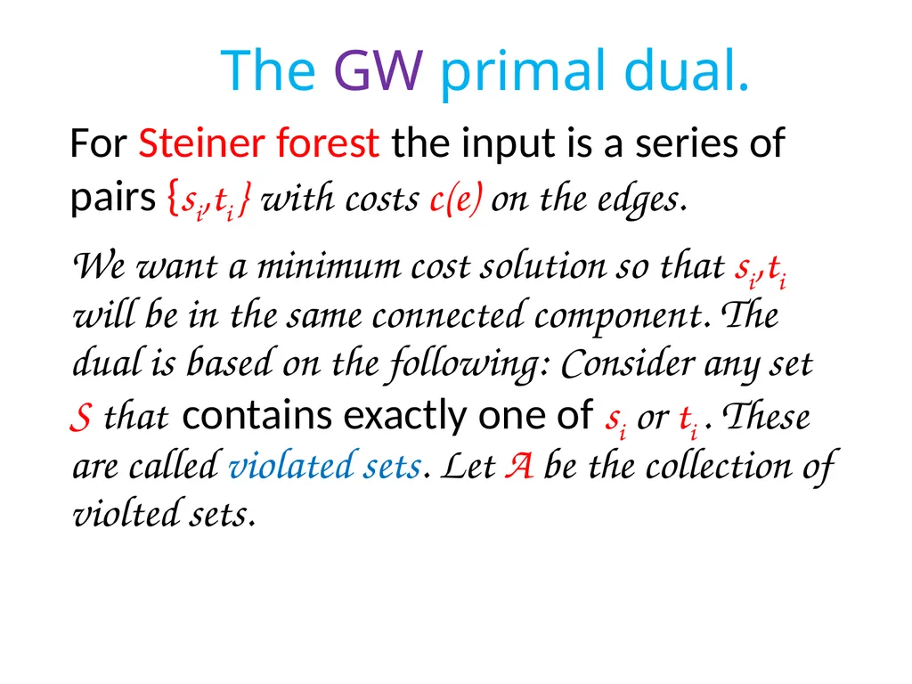
slide2. The GW primal dual. For Steiner forest the input is a series of pairs {si,ti } with costs c(e) on the edges.
We want a minimum cost solution so that si,ti will be in the same connected component. The dual is based on the following: Consider any set S that contains exactly one of si or ti . These are called violated sets. Let A be the collection of violted sets.<br>
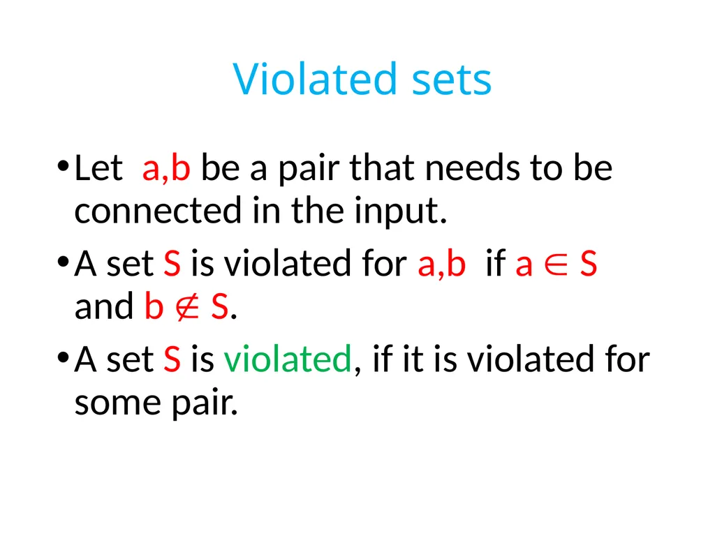
slide3. Violated sets Let a,b be a pair that needs to be connected in the input.
A set S is violated for a,b if a S and b S.
A set S is violated, if it is violated for some pair.<br>
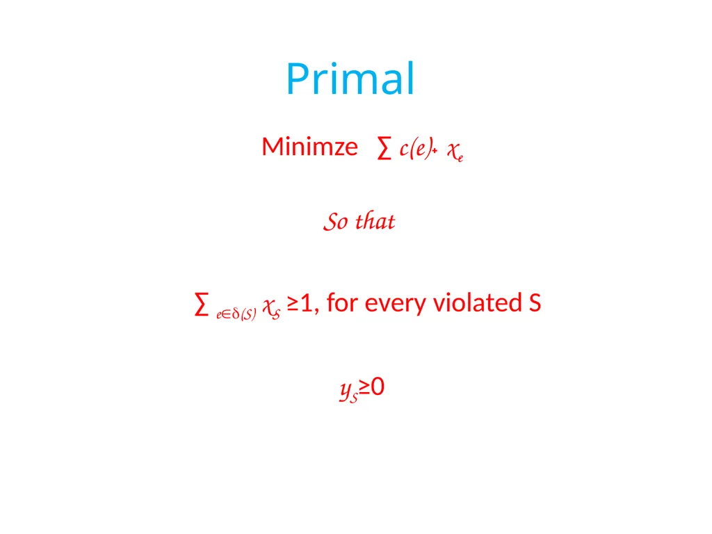
slide4. Primal Minimze ∑ c(e)˖ xe
So that
∑ e(S) xS ≥1, for every violated S
yS≥0<br>
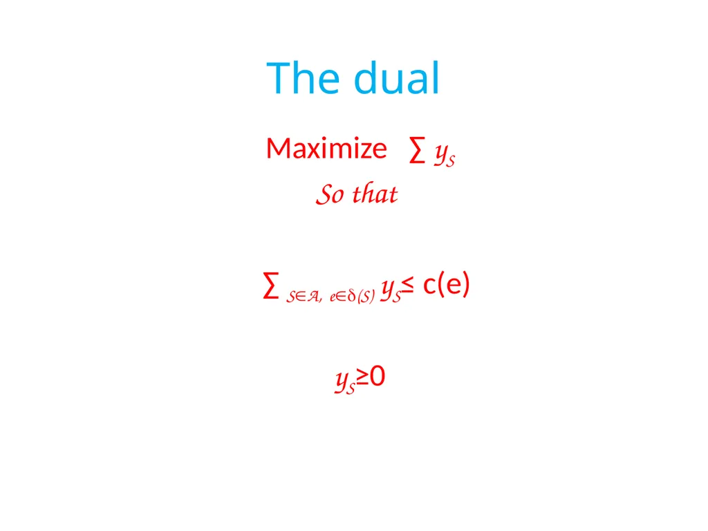
slide5. The dual Maximize ∑ yS
So that
∑ SA, e(S) yS≤ c(e)
yS≥0<br>
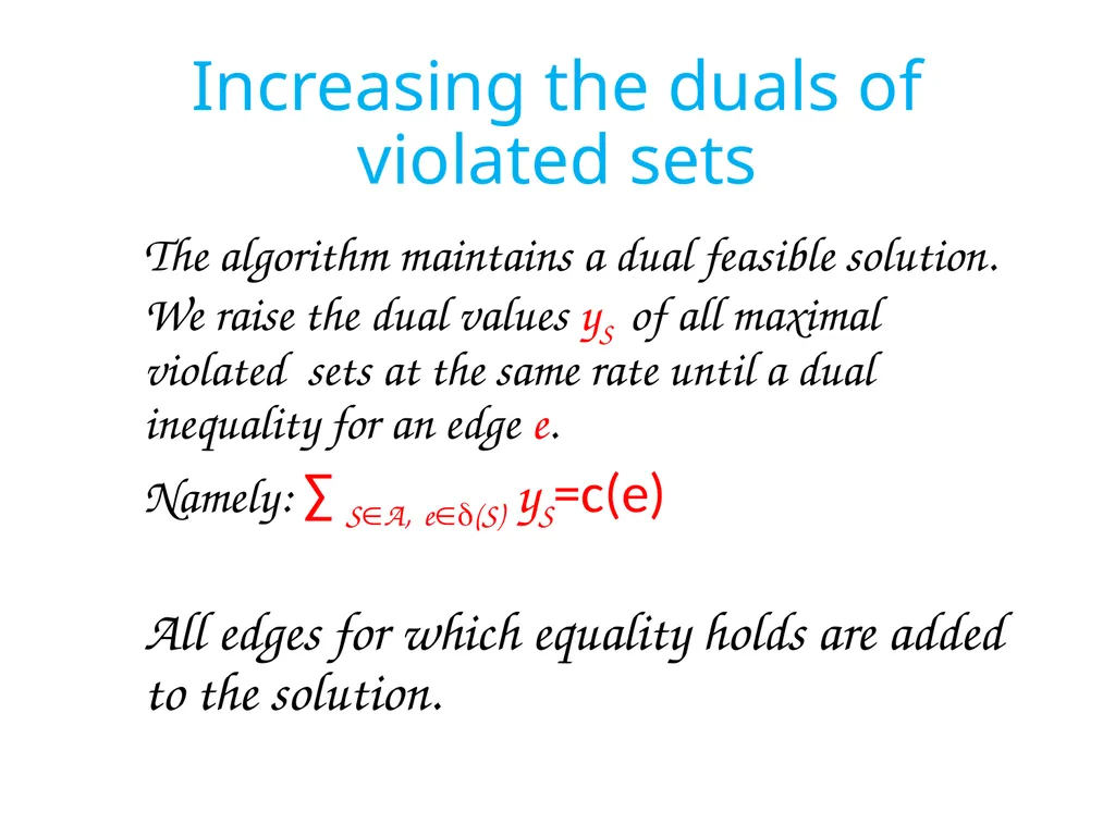
slide6. Increasing the duals of violated sets The algorithm maintains a dual feasible solution. We raise the dual values yS of all maximal violated sets at the same rate until a dual inequality for an edge e.
Namely: ∑ SA, e(S) yS=c(e)
All edges for which equality holds are added to the solution.<br>
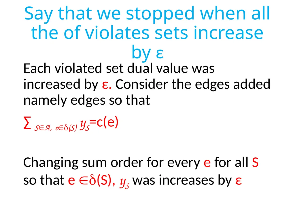
slide7. Say that we stopped when all the of violates sets increase by ε Each violated set dual value was increased by ε. Consider the edges added namely edges so that
∑ SA, e(S) yS=c(e)
Changing sum order for every e for all S so that e (S), yS was increases by ε<br>
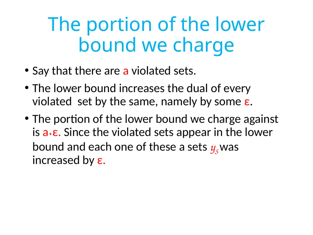
slide8. The portion of the lower bound we charge Say that there are a violated sets.
The lower bound increases the dual of every violated set by the same, namely by some ε.
The portion of the lower bound we charge against is a˖ε. Since the violated sets appear in the lower bound and each one of these a sets yS was increased by ε.<br>
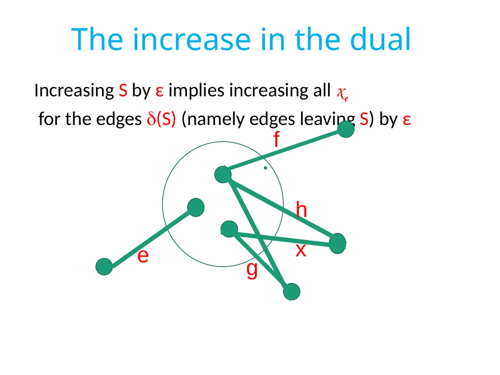
slide9. The increase in the dual Increasing S by ε implies increasing all xe
for the edges (S) (namely edges leaving S) by ε e f h x g<br>
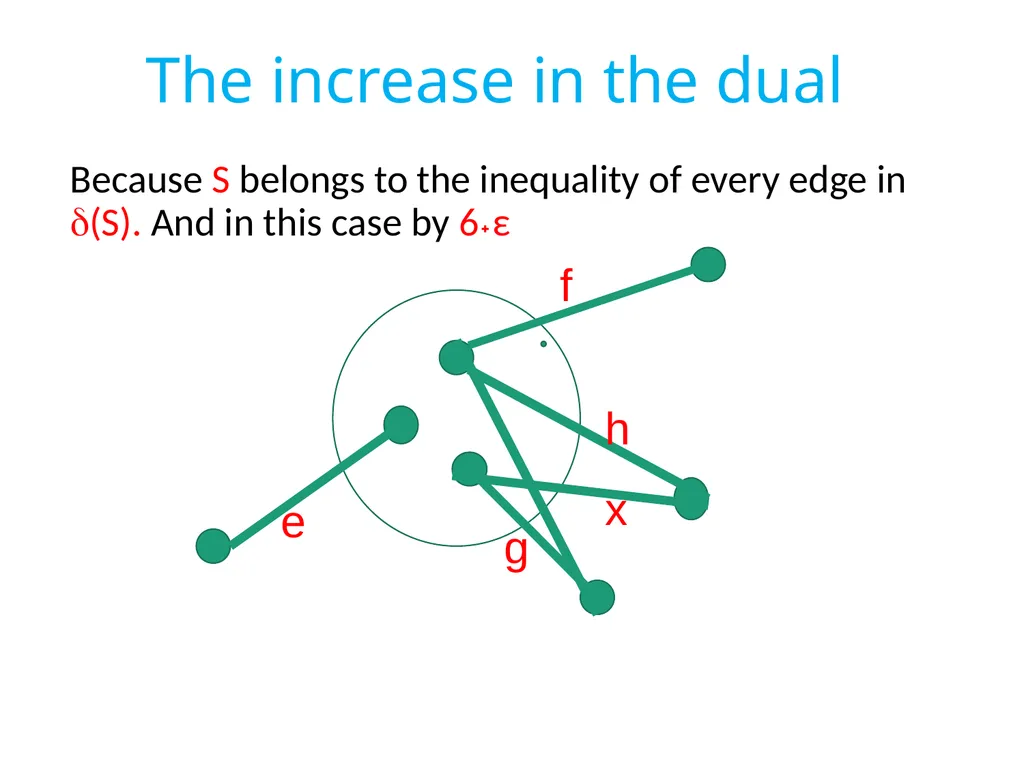
slide10. The increase in the dual Because S belongs to the inequality of every edge in (S). And in this case by 6˖ε e f h x g<br>
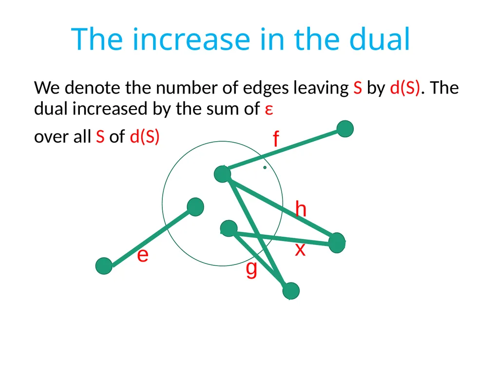
slide11. The increase in the dual We denote the number of edges leaving S by d(S). The dual increased by the sum of ε
over all S of d(S) e f h x g<br>
slide12. Making the edges a forest on violated and non violated sets We can (reverse) delete edges and keep connectivity.
Hence the edges chosen and not deleted form a forest on violated and non violated sets. The increase in our dual is by
∑SA d(S)˖ε with d(S) the number of edges leaving S. This needs to be compared to a˖ε<br>
slide13. The average degree The thing that determines the ratio is therefore ∑ d(s)/a namely, the average degree of violated sets.
For this it is useful to note that leaves are violated sets. If a leaf is not violated, the unique edge can be removed and the solution is still feasible.<br>
slide14. The average degree of violated sets The sum of degrees in this tree is 2k-2 with k the number of violated and non violated sets, and so the average is 2-2/k.
Now, what happens when we ignore non volated sets?
Since each non violated set is not a leaf it’s degree is at least 2 namely above the average. Hence removing non violated sets can only decrease the average.
And so the average of violated sets is at most 2-2/k.
Since the sum of degrees of violated sets is the contribution to the dual, and a˖ε is the part of the lower bound we charge, the approximation ratio is at most 2-2/k<br>
slide15. What did we do? The cost of edges were “broken” into uniform values with different fixed ε.
For every such increase we show that the increase in the dual of of violated sets is at least ½ the increase in the dual.
Hence each event ratio 2. Hence ratio 2.<br>
slide2. The GW primal dual. For Steiner forest the input is a series of pairs {si,ti } with costs c(e) on the edges.
We want a minimum cost solution so that si,ti will be in the same connected component. The dual is based on the following: Consider any set S that contains exactly one of si or ti . These are called violated sets. Let A be the collection of violted sets.<br>
slide3. Violated sets Let a,b be a pair that needs to be connected in the input.
A set S is violated for a,b if a S and b S.
A set S is violated, if it is violated for some pair.<br>
slide4. Primal Minimze ∑ c(e)˖ xe
So that
∑ e(S) xS ≥1, for every violated S
yS≥0<br>
slide5. The dual Maximize ∑ yS
So that
∑ SA, e(S) yS≤ c(e)
yS≥0<br>
slide6. Increasing the duals of violated sets The algorithm maintains a dual feasible solution. We raise the dual values yS of all maximal violated sets at the same rate until a dual inequality for an edge e.
Namely: ∑ SA, e(S) yS=c(e)
All edges for which equality holds are added to the solution.<br>
slide7. Say that we stopped when all the of violates sets increase by ε Each violated set dual value was increased by ε. Consider the edges added namely edges so that
∑ SA, e(S) yS=c(e)
Changing sum order for every e for all S so that e (S), yS was increases by ε<br>
slide8. The portion of the lower bound we charge Say that there are a violated sets.
The lower bound increases the dual of every violated set by the same, namely by some ε.
The portion of the lower bound we charge against is a˖ε. Since the violated sets appear in the lower bound and each one of these a sets yS was increased by ε.<br>
slide9. The increase in the dual Increasing S by ε implies increasing all xe
for the edges (S) (namely edges leaving S) by ε e f h x g<br>
slide10. The increase in the dual Because S belongs to the inequality of every edge in (S). And in this case by 6˖ε e f h x g<br>
slide11. The increase in the dual We denote the number of edges leaving S by d(S). The dual increased by the sum of ε
over all S of d(S) e f h x g<br>
slide12. Making the edges a forest on violated and non violated sets We can (reverse) delete edges and keep connectivity.
Hence the edges chosen and not deleted form a forest on violated and non violated sets. The increase in our dual is by
∑SA d(S)˖ε with d(S) the number of edges leaving S. This needs to be compared to a˖ε<br>
slide13. The average degree The thing that determines the ratio is therefore ∑ d(s)/a namely, the average degree of violated sets.
For this it is useful to note that leaves are violated sets. If a leaf is not violated, the unique edge can be removed and the solution is still feasible.<br>
slide14. The average degree of violated sets The sum of degrees in this tree is 2k-2 with k the number of violated and non violated sets, and so the average is 2-2/k.
Now, what happens when we ignore non volated sets?
Since each non violated set is not a leaf it’s degree is at least 2 namely above the average. Hence removing non violated sets can only decrease the average.
And so the average of violated sets is at most 2-2/k.
Since the sum of degrees of violated sets is the contribution to the dual, and a˖ε is the part of the lower bound we charge, the approximation ratio is at most 2-2/k<br>
slide15. What did we do? The cost of edges were “broken” into uniform values with different fixed ε.
For every such increase we show that the increase in the dual of of violated sets is at least ½ the increase in the dual.
Hence each event ratio 2. Hence ratio 2.<br>