Basic Concepts from Economics © 2018 D. Kirschen

slide1. Basic Concepts from Economics © 2018 D. Kirschen and the University of Washington 1<br>
slide2. Let us go to the market... © 2018 D. Kirschen and the University of Washington 2 Opportunity for buyers and sellers to:
compare prices
estimate demand
estimate supply

Achieve an equilibrium between supply and demand<br>
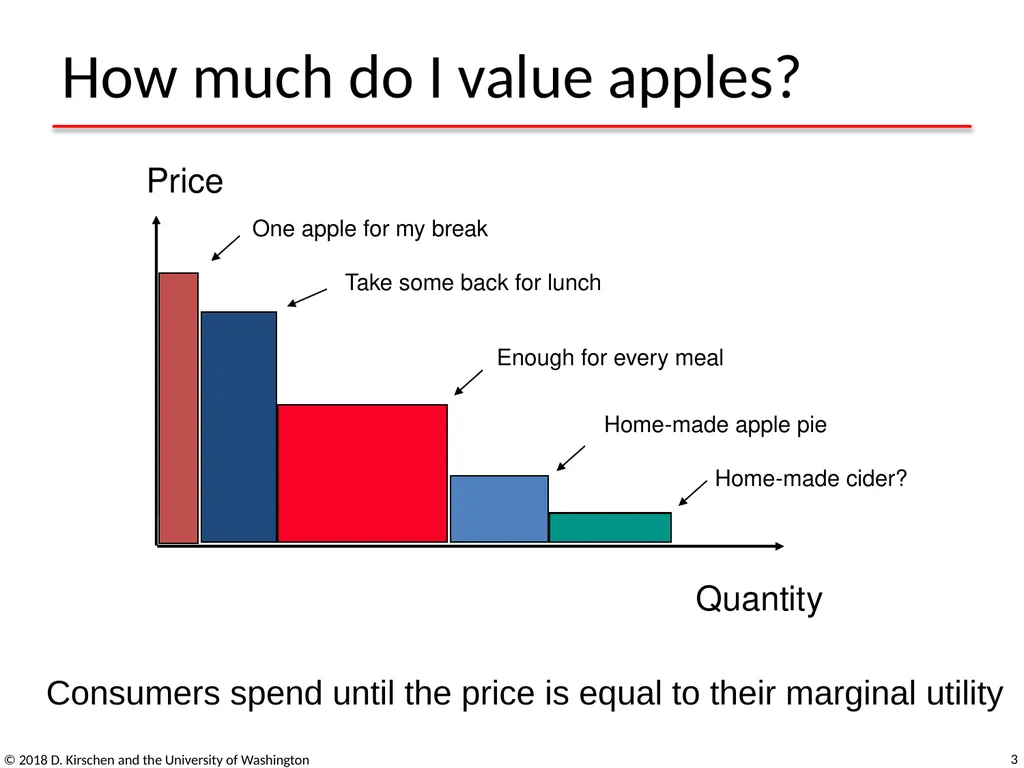
slide3. How much do I value apples? © 2018 D. Kirschen and the University of Washington 3 Consumers spend until the price is equal to their marginal utility<br>
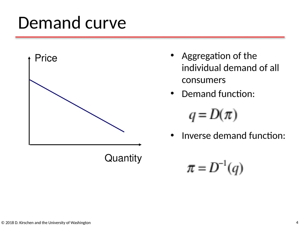
slide4. Demand curve © 2018 D. Kirschen and the University of Washington 4 Aggregation of the individual demand of all consumers
Demand function:

Inverse demand function:<br>
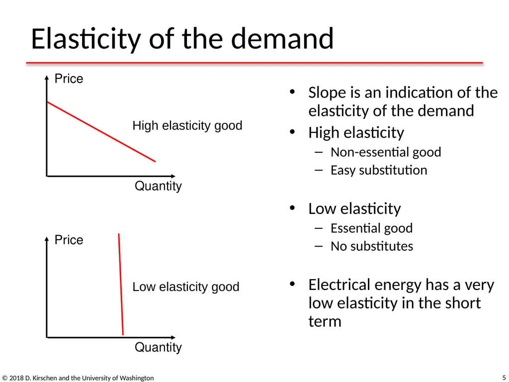
slide5. Elasticity of the demand © 2018 D. Kirschen and the University of Washington 5 Slope is an indication of the elasticity of the demand
High elasticity
Non-essential good
Easy substitution

Low elasticity
Essential good
No substitutes

Electrical energy has a very low elasticity in the short term Price Quantity Low elasticity good High elasticity good<br>
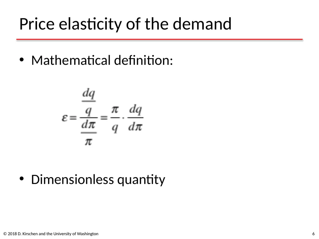
slide6. Price elasticity of the demand Mathematical definition:

Dimensionless quantity © 2018 D. Kirschen and the University of Washington 6<br>
slide7. Supply side How many widgets shall I produce?
Goal: make a profit on each widget sold
Produce one more widget if and only if the cost of producing it is less than the market price

Need to know the cost of producing the next widget
Considers only the variable costs
Ignores the fixed costs
Investments in production plants and machines © 2018 D. Kirschen and the University of Washington 7<br>
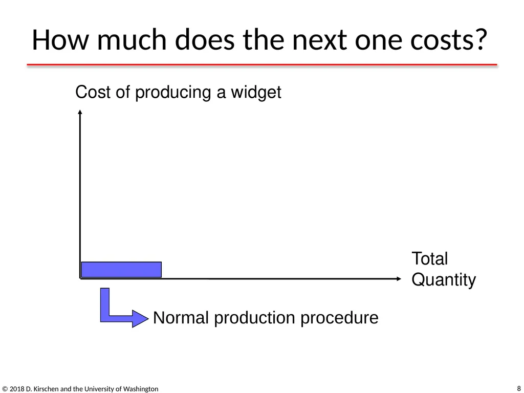
slide8. How much does the next one costs? © 2018 D. Kirschen and the University of Washington 8 Cost of producing a widget Total
Quantity Normal production procedure<br>
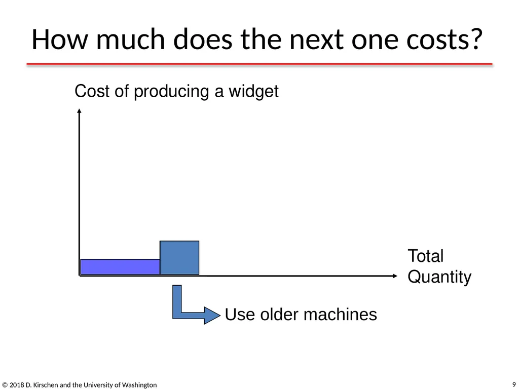
slide9. How much does the next one costs? © 2018 D. Kirschen and the University of Washington 9 Cost of producing a widget Total
Quantity Use older machines<br>
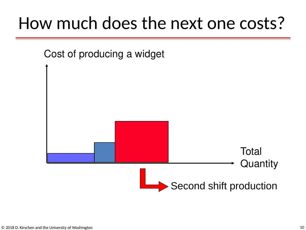
slide10. How much does the next one costs? © 2018 D. Kirschen and the University of Washington 10 Cost of producing a widget Total
Quantity Second shift production<br>
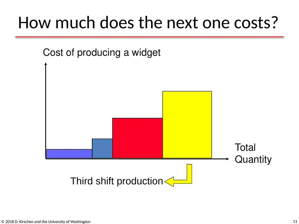
slide11. How much does the next one costs? © 2018 D. Kirschen and the University of Washington 11 Cost of producing a widget Total
Quantity Third shift production<br>
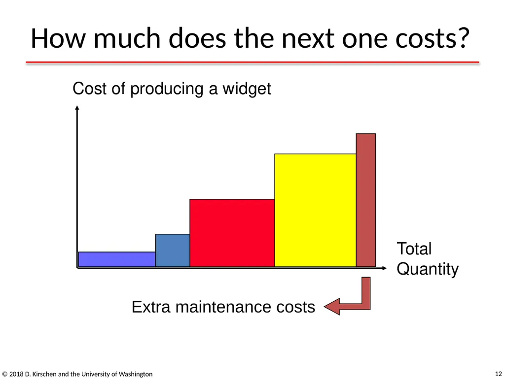
slide12. How much does the next one costs? © 2018 D. Kirschen and the University of Washington 12 Cost of producing a widget Total
Quantity Extra maintenance costs<br>
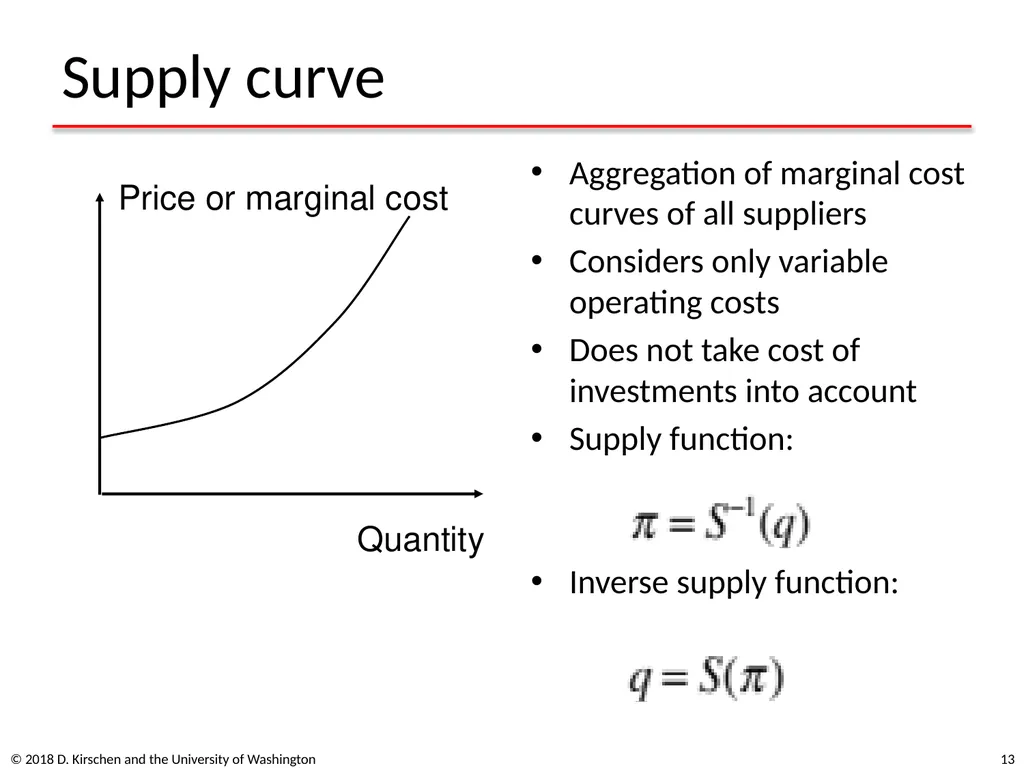
slide13. Supply curve Aggregation of marginal cost curves of all suppliers
Considers only variable operating costs
Does not take cost of investments into account
Supply function:

Inverse supply function: © 2018 D. Kirschen and the University of Washington 13<br>
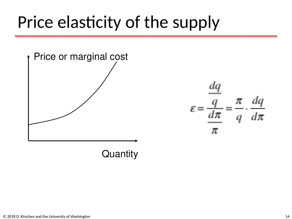
slide14. Price elasticity of the supply © 2018 D. Kirschen and the University of Washington 14<br>
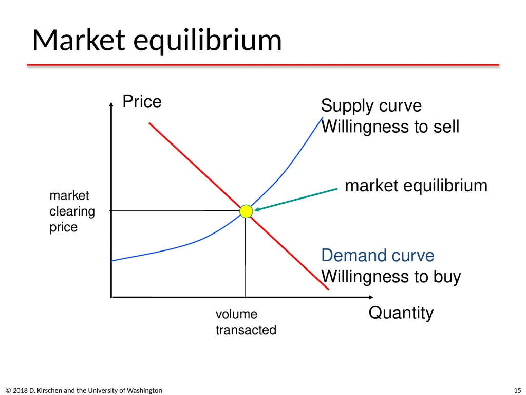
slide15. Market equilibrium © 2018 D. Kirschen and the University of Washington 15<br>
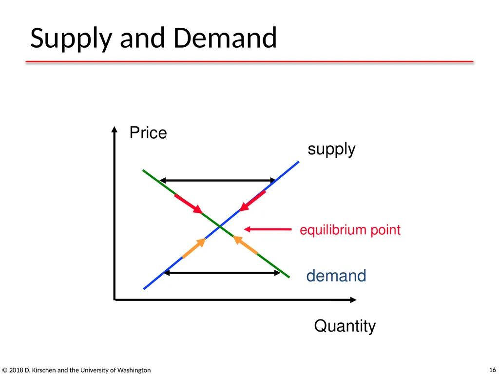
slide16. Supply and Demand © 2018 D. Kirschen and the University of Washington 16 Price Quantity supply demand equilibrium point<br>
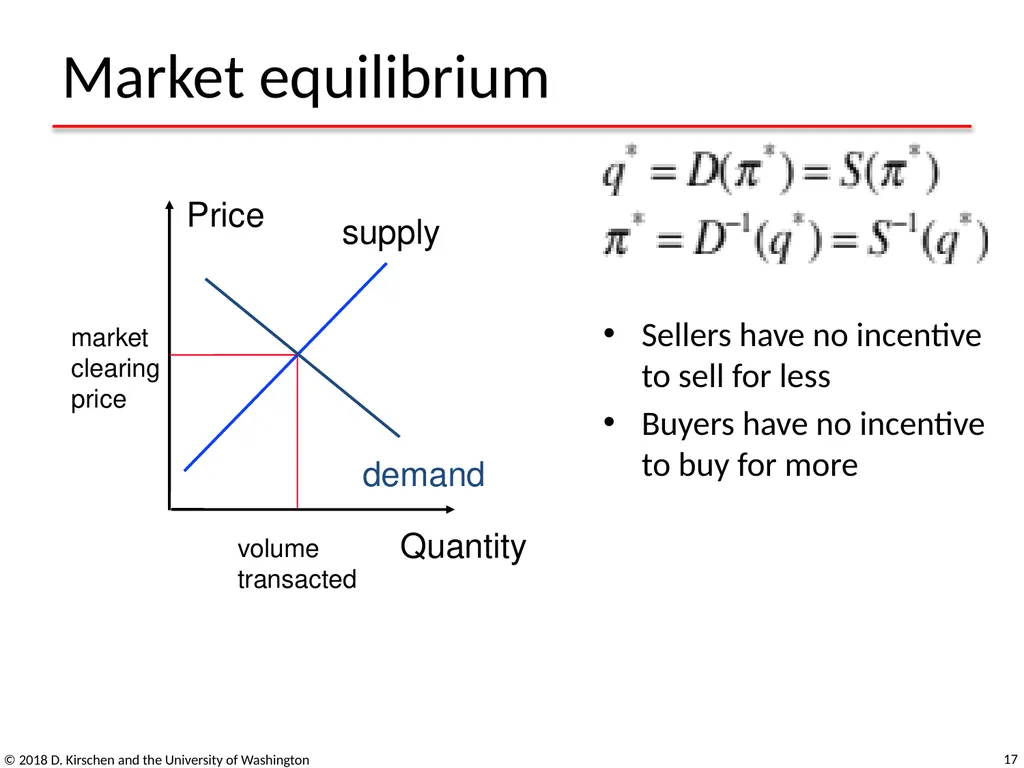
slide17. Market equilibrium © 2018 D. Kirschen and the University of Washington 17 Sellers have no incentive to sell for less
Buyers have no incentive to buy for more<br>
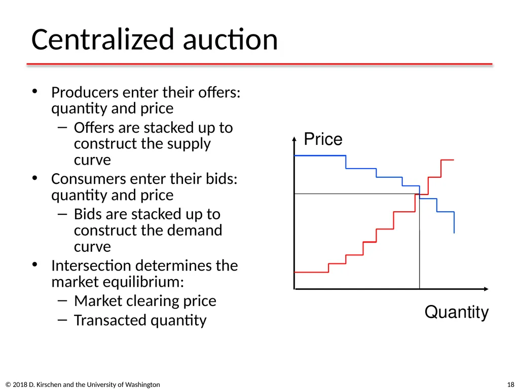
slide18. Centralized auction Producers enter their offers: quantity and price
Offers are stacked up to construct the supply curve
Consumers enter their bids: quantity and price
Bids are stacked up to construct the demand curve
Intersection determines the market equilibrium:
Market clearing price
Transacted quantity © 2018 D. Kirschen and the University of Washington 18<br>
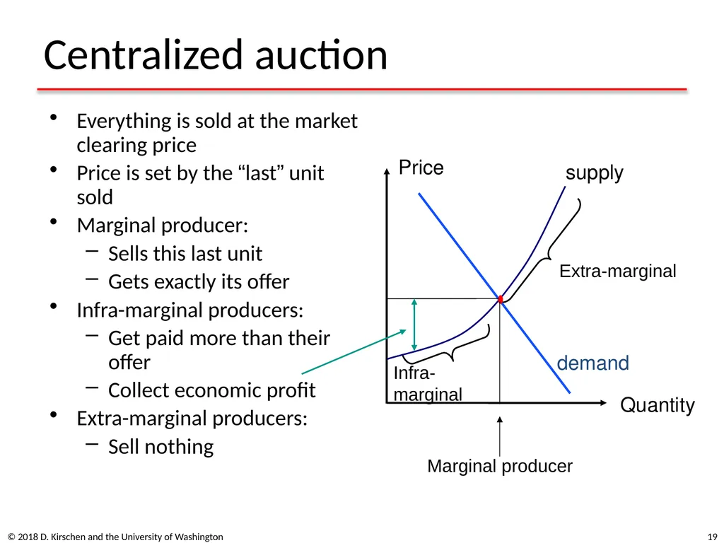
slide19. Centralized auction Everything is sold at the market clearing price
Price is set by the “last” unit sold
Marginal producer:
Sells this last unit
Gets exactly its offer
Infra-marginal producers:
Get paid more than their offer
Collect economic profit
Extra-marginal producers:
Sell nothing © 2018 D. Kirschen and the University of Washington 19<br>
slide20. Bilateral transactions Producers and consumers trade directly and independently
Consumers “shop around” for the best deal
Producers check the competition’s prices
An efficient market “discovers” the equilibrium price © 2018 D. Kirschen and the University of Washington 20<br>
slide21. What makes a market efficient? All buyers and sellers have access to sufficient information about prices, supply and demand
Factors favouring an efficient market
Number of participants
Standard definition of commodities
Good information exchange mechanisms © 2018 D. Kirschen and the University of Washington 21<br>
slide22. Examples Efficient markets:
Open air food market
Chicago mercantile exchange
Inefficient markets:
Used cars © 2018 D. Kirschen and the University of Washington 22<br>
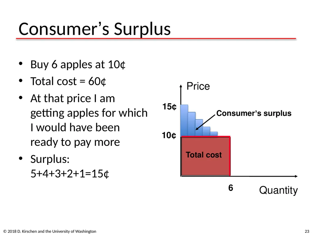
slide23. Consumer’s Surplus Buy 6 apples at 10¢
Total cost = 60¢
At that price I am getting apples for which I would have been ready to pay more
Surplus: 5+4+3+2+1=15¢ © 2018 D. Kirschen and the University of Washington 23 15¢ 10¢ 6<br>
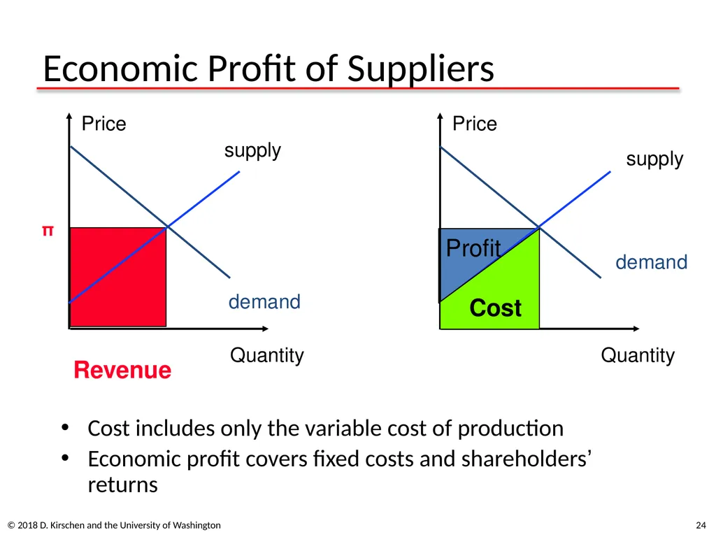
slide24. Economic Profit of Suppliers Cost includes only the variable cost of production
Economic profit covers fixed costs and shareholders’ returns © 2018 D. Kirschen and the University of Washington 24<br>
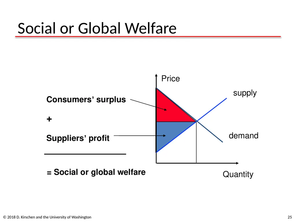
slide25. Social or Global Welfare © 2018 D. Kirschen and the University of Washington 25<br>
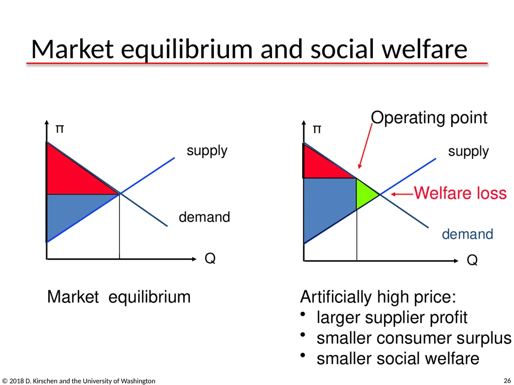
slide26. Market equilibrium and social welfare © 2018 D. Kirschen and the University of Washington 26 Market equilibrium Artificially high price:
larger supplier profit
smaller consumer surplus
smaller social welfare Q π supply demand Welfare loss Operating point<br>
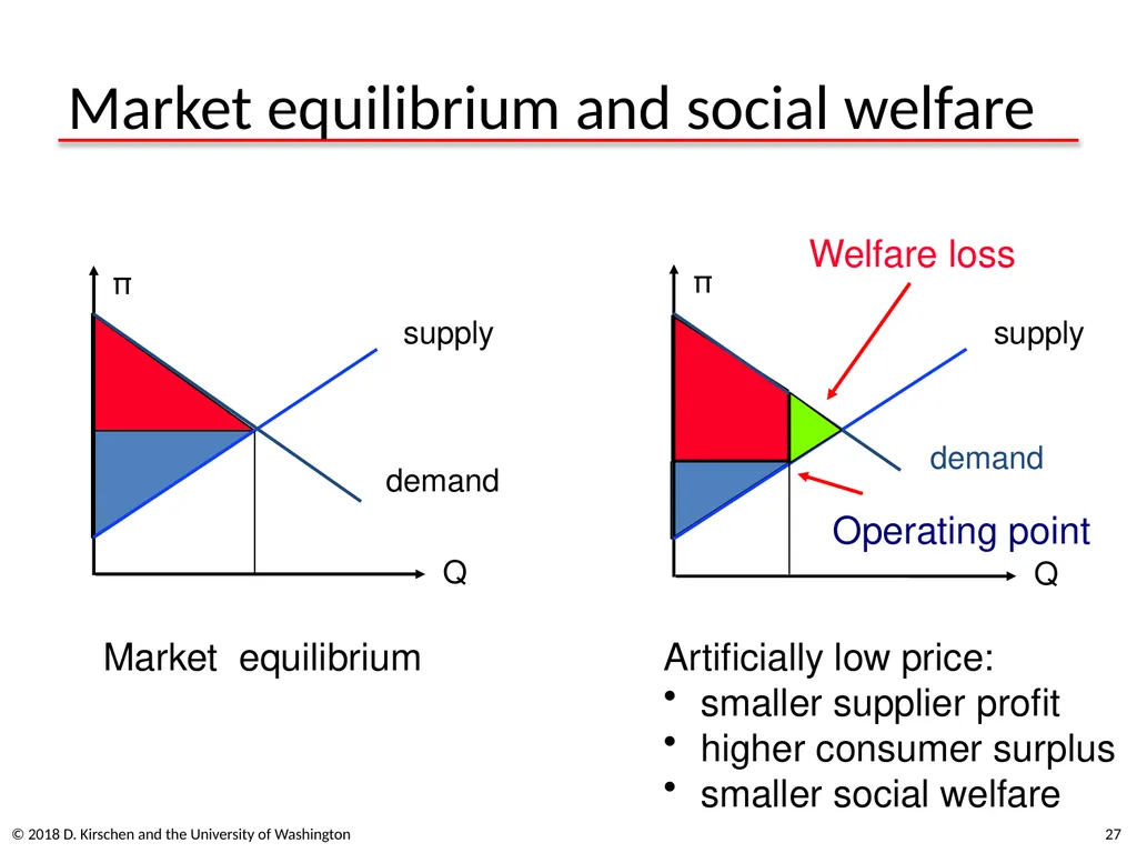
slide27. Market equilibrium and social welfare © 2018 D. Kirschen and the University of Washington 27 Q π supply demand Market equilibrium Artificially low price:
smaller supplier profit
higher consumer surplus
smaller social welfare Welfare loss Operating point<br>
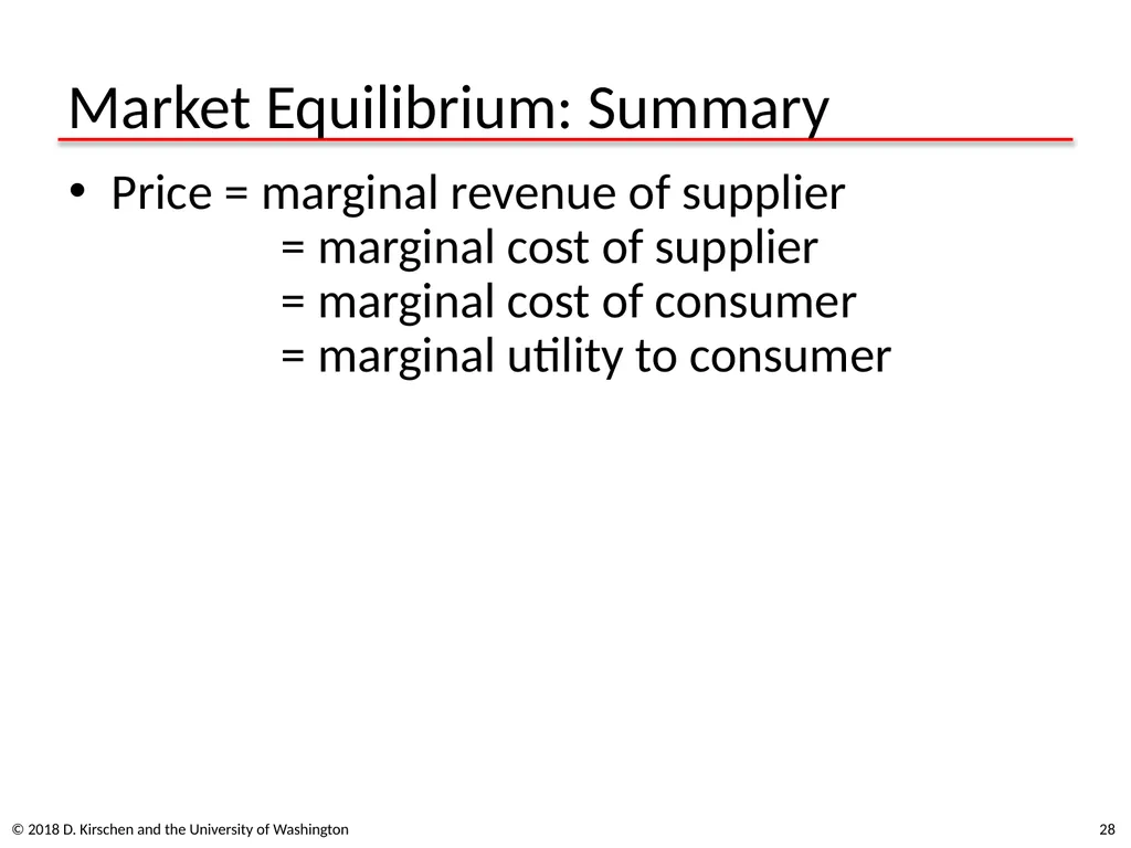
slide28. Market Equilibrium: Summary Price = marginal revenue of supplier = marginal cost of supplier = marginal cost of consumer = marginal utility to consumer © 2018 D. Kirschen and the University of Washington 28<br>
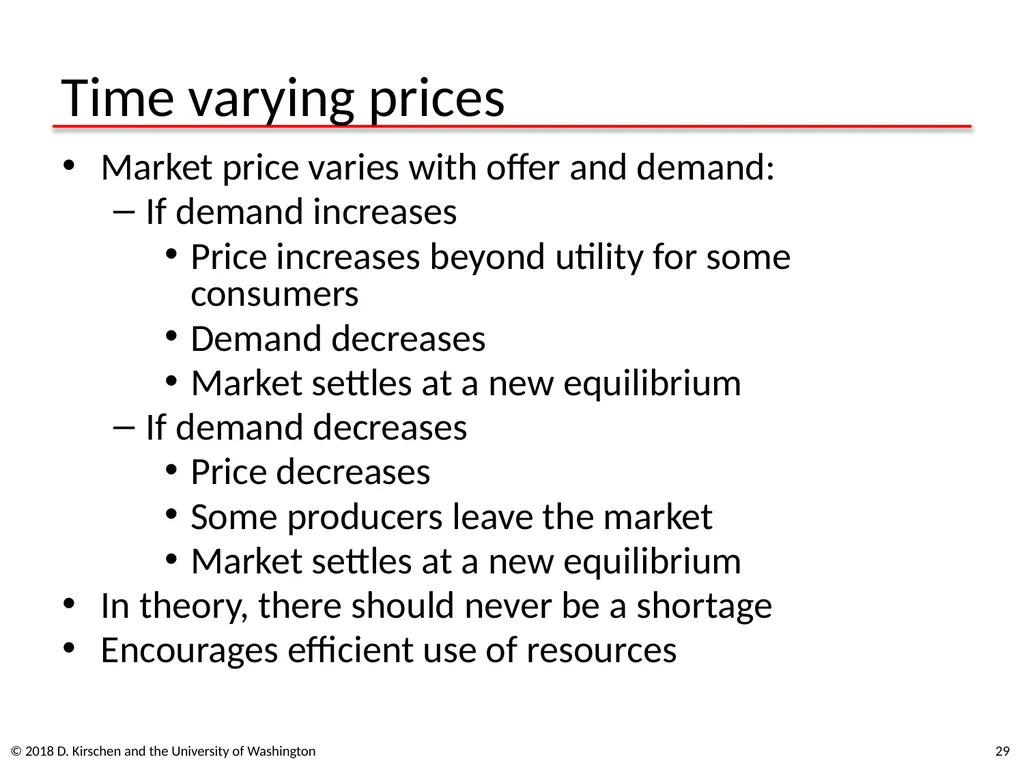
slide29. Time varying prices Market price varies with offer and demand:
If demand increases
Price increases beyond utility for some consumers
Demand decreases
Market settles at a new equilibrium
If demand decreases
Price decreases
Some producers leave the market
Market settles at a new equilibrium
In theory, there should never be a shortage
Encourages efficient use of resources © 2018 D. Kirschen and the University of Washington 29<br>
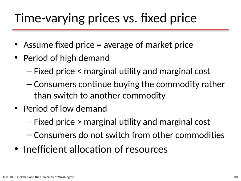
slide30. Time-varying prices vs. fixed price Assume fixed price = average of market price
Period of high demand
Fixed price < marginal utility and marginal cost
Consumers continue buying the commodity rather than switch to another commodity
Period of low demand
Fixed price > marginal utility and marginal cost
Consumers do not switch from other commodities
Inefficient allocation of resources © 2018 D. Kirschen and the University of Washington 30<br>
slide31. Concepts from the Theory of the Firm © 2018 D. Kirschen and the University of Washington 31<br>
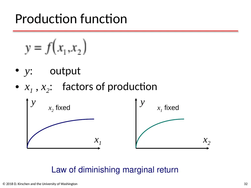
slide32. Production function y: output
x1 , x2: factors of production © 2018 D. Kirschen and the University of Washington 32 y Law of diminishing marginal return<br>
slide33. Long run and short run Some factors of production can be adjusted faster than others
Example: fertilizer vs. planting more trees
Long run: all factors can be changed
Short run: some factors cannot be changed
No specific duration separates long and short run
Long run = long term
Short run = short term © 2018 D. Kirschen and the University of Washington 33<br>
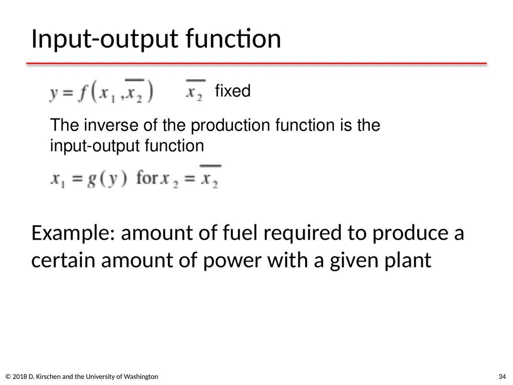
slide34. Input-output function Example: amount of fuel required to produce a certain amount of power with a given plant © 2018 D. Kirschen and the University of Washington 34 fixed The inverse of the production function is the
input-output function<br>
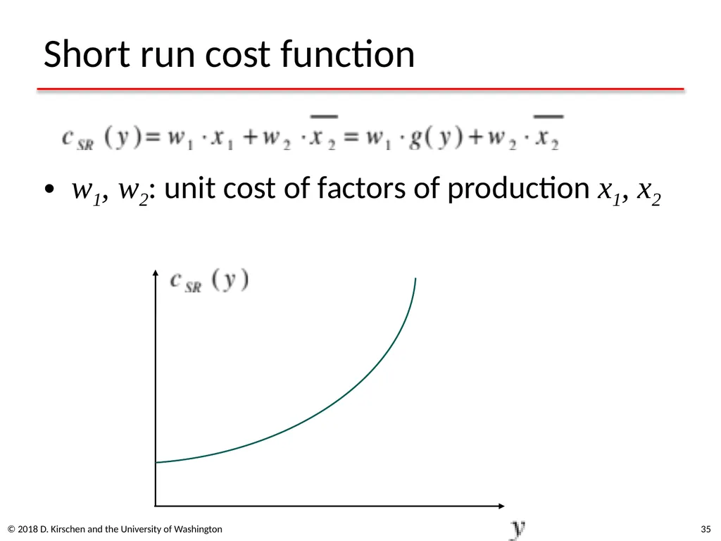
slide35. Short run cost function w1, w2: unit cost of factors of production x1, x2 © 2018 D. Kirschen and the University of Washington 35<br>
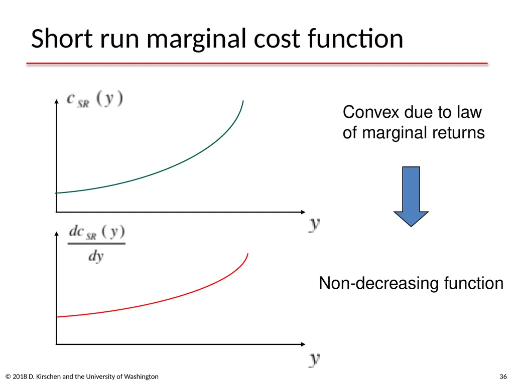
slide36. Short run marginal cost function © 2018 D. Kirschen and the University of Washington 36 Convex due to law
of marginal returns Non-decreasing function<br>
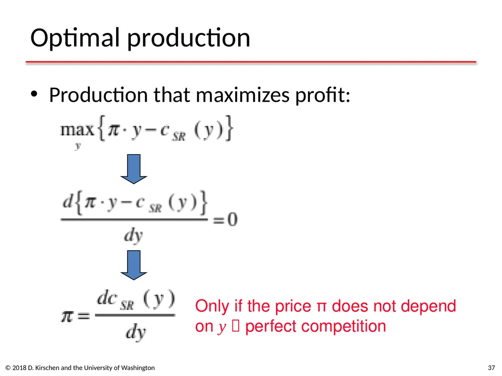
slide37. Optimal production Production that maximizes profit: © 2018 D. Kirschen and the University of Washington 37 Only if the price π does not depend
on y  perfect competition<br>
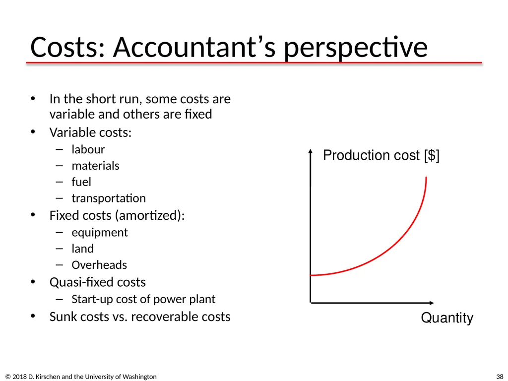
slide38. Costs: Accountant’s perspective In the short run, some costs are variable and others are fixed
Variable costs:
labour
materials
fuel
transportation
Fixed costs (amortized):
equipment
land
Overheads
Quasi-fixed costs
Start-up cost of power plant
Sunk costs vs. recoverable costs © 2018 D. Kirschen and the University of Washington 38<br>
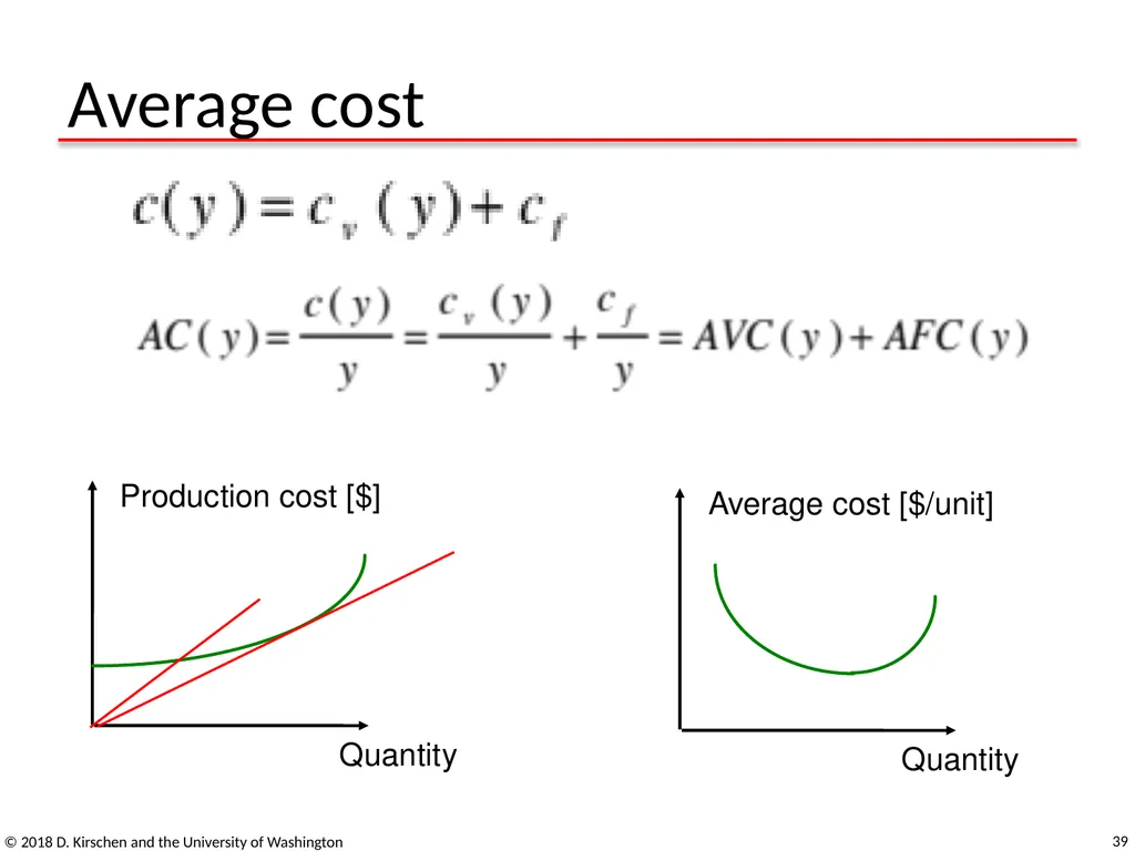
slide39. Average cost © 2018 D. Kirschen and the University of Washington 39 Quantity Production cost [$] Quantity Average cost [$/unit]<br>
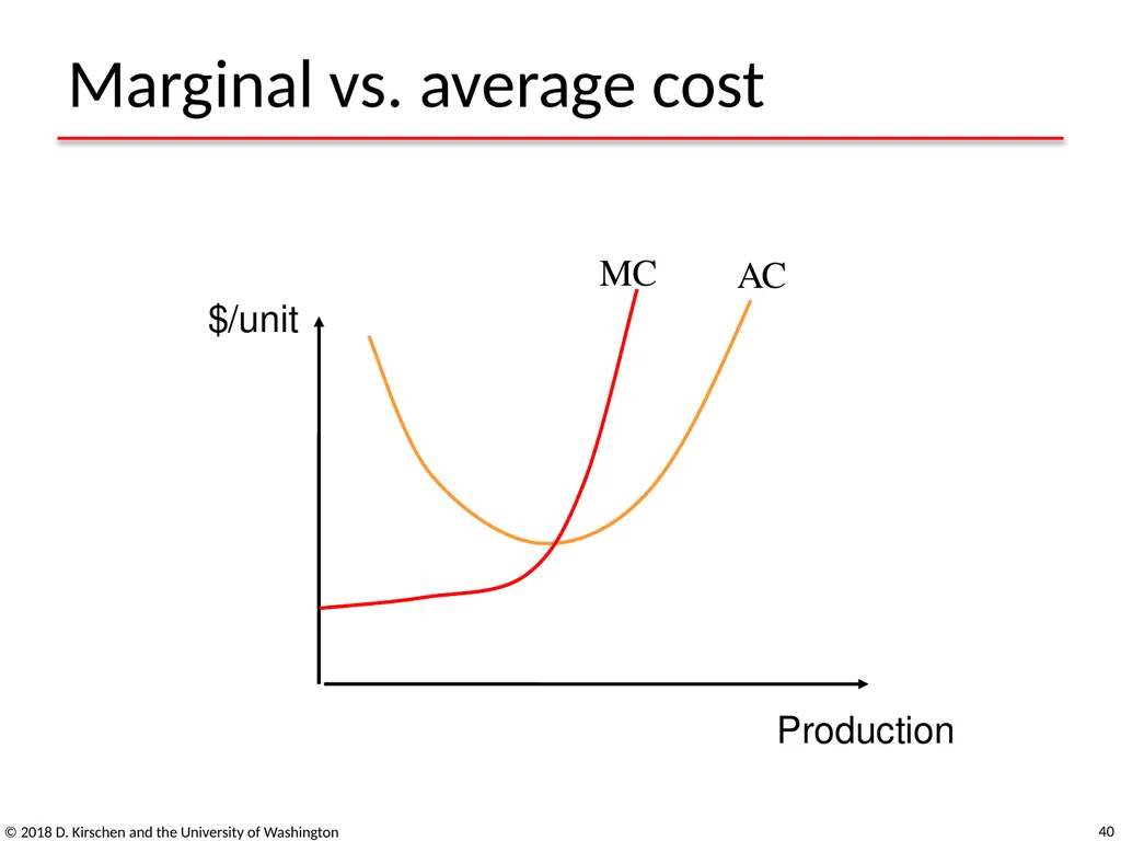
slide40. Marginal vs. average cost © 2018 D. Kirschen and the University of Washington 40 MC AC $/unit Production<br>
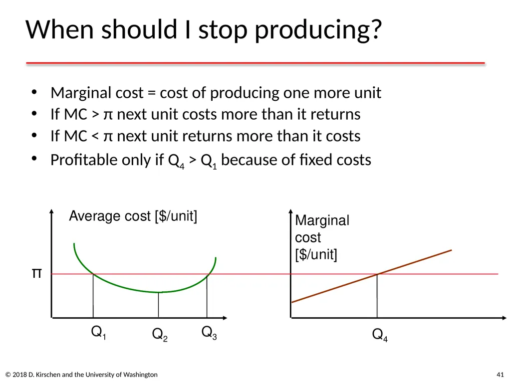
slide41. When should I stop producing? Marginal cost = cost of producing one more unit
If MC > π next unit costs more than it returns
If MC < π next unit returns more than it costs
Profitable only if Q4 > Q1 because of fixed costs © 2018 D. Kirschen and the University of Washington 41 Marginal
cost
[$/unit] Average cost [$/unit] π Q1 Q3 Q4 Q2<br>
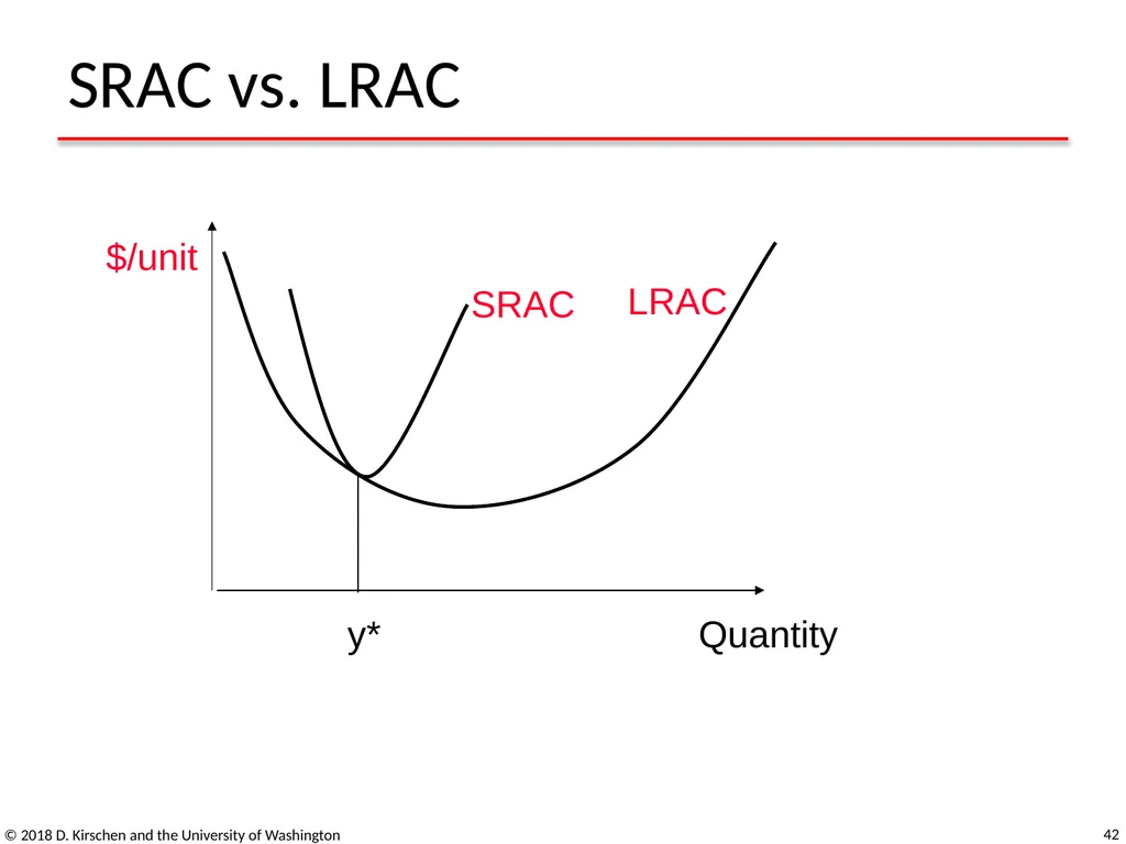
slide42. SRAC vs. LRAC © 2018 D. Kirschen and the University of Washington 42 $/unit LRAC SRAC Quantity y*<br>
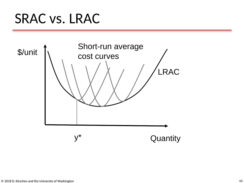
slide43. SRAC vs. LRAC © 2018 D. Kirschen and the University of Washington 43 $/unit LRAC Short-run average cost curves Quantity y*<br>
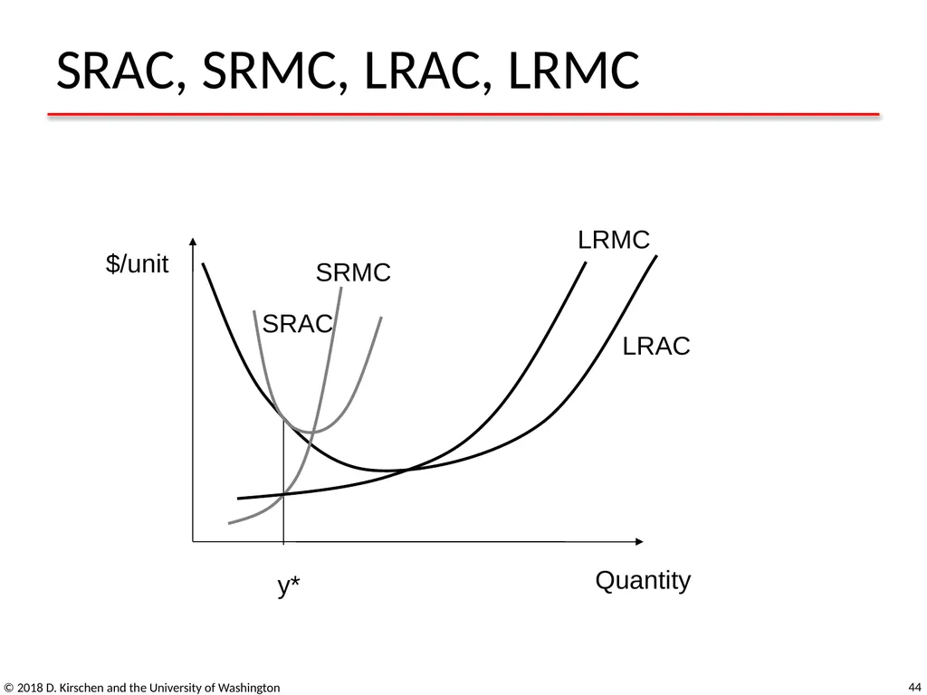
slide44. SRAC, SRMC, LRAC, LRMC © 2018 D. Kirschen and the University of Washington 44 $/unit LRAC SRAC SRMC LRMC Quantity y*<br>
slide45. Costs: Economist’s perspective Opportunity cost:
What would be the best use of the money spent to make the product ?
Not taking the opportunity to sell at a higher price represents a cost
Examples:
Use the money to grow apples or put it in the bank where it earns interests?
Growing apples or growing kiwis?
Comparisons should be made against a “normal profit”
What putting money in the bank would bring
Selling “at cost” means making a “normal profit”
Usually not good enough because it does not compensate for the risk involved in the business © 2018 D. Kirschen and the University of Washington 45<br>
slide46. Risks, Markets and Contracts 46<br>
slide47. Concept of Risk Future is uncertain
Uncertainty translates into risk
In this case, risk of loss of income
Risk = probability x consequences
Doing business means accepting some risks
Willingness to accept risk varies:
Venture capitalist vs. retiree
Ability to control risk varies:
Professional traders vs. novice investors 47 © 2018 D. Kirschen and the University of Washington<br>
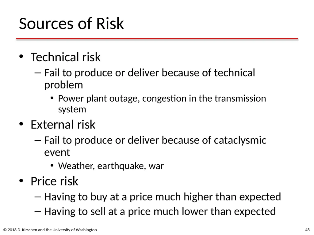
slide48. Sources of Risk Technical risk
Fail to produce or deliver because of technical problem
Power plant outage, congestion in the transmission system
External risk
Fail to produce or deliver because of cataclysmic event
Weather, earthquake, war
Price risk
Having to buy at a price much higher than expected
Having to sell at a price much lower than expected 48 © 2018 D. Kirschen and the University of Washington<br>
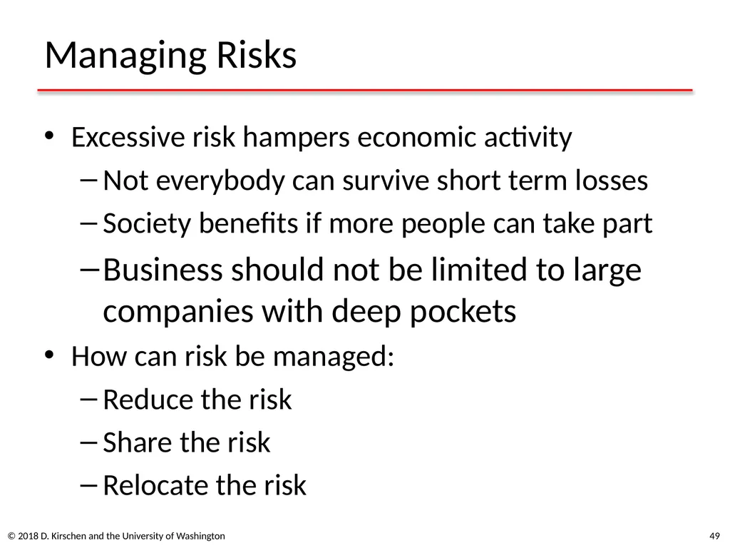
slide49. Managing Risks Excessive risk hampers economic activity
Not everybody can survive short term losses
Society benefits if more people can take part
Business should not be limited to large companies with deep pockets
How can risk be managed:
Reduce the risk
Share the risk
Relocate the risk 49 © 2018 D. Kirschen and the University of Washington<br>
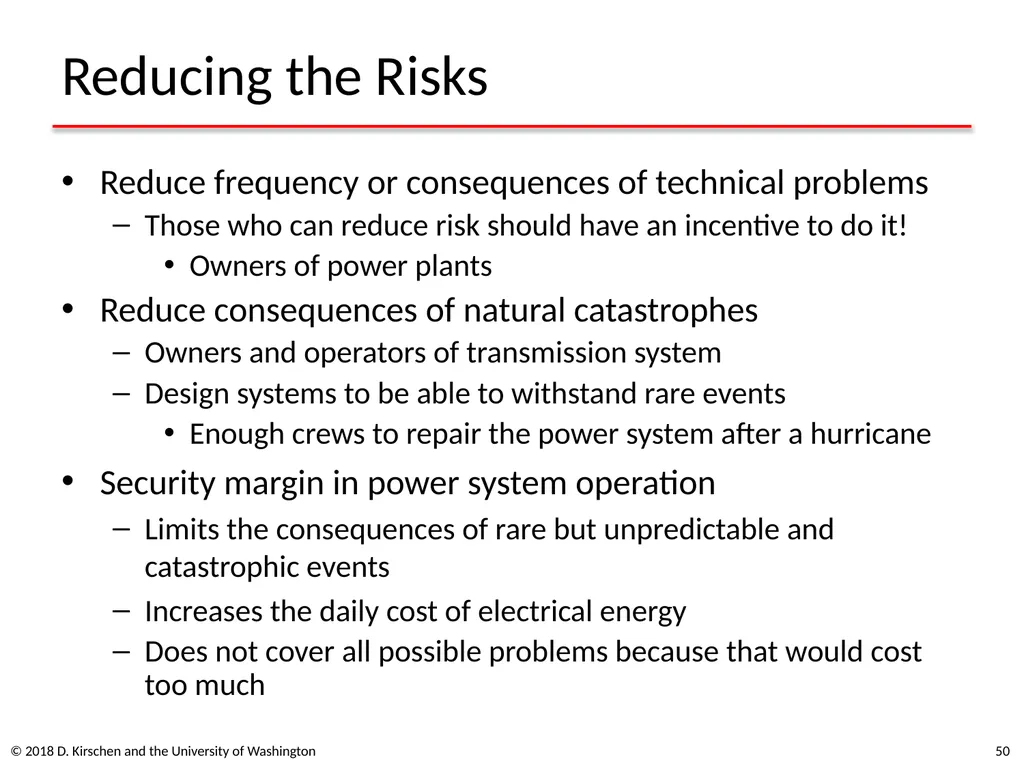
slide50. Reducing the Risks Reduce frequency or consequences of technical problems
Those who can reduce risk should have an incentive to do it!
Owners of power plants
Reduce consequences of natural catastrophes
Owners and operators of transmission system
Design systems to be able to withstand rare events
Enough crews to repair the power system after a hurricane
Security margin in power system operation
Limits the consequences of rare but unpredictable and catastrophic events
Increases the daily cost of electrical energy
Does not cover all possible problems because that would cost too much 50 © 2018 D. Kirschen and the University of Washington<br>
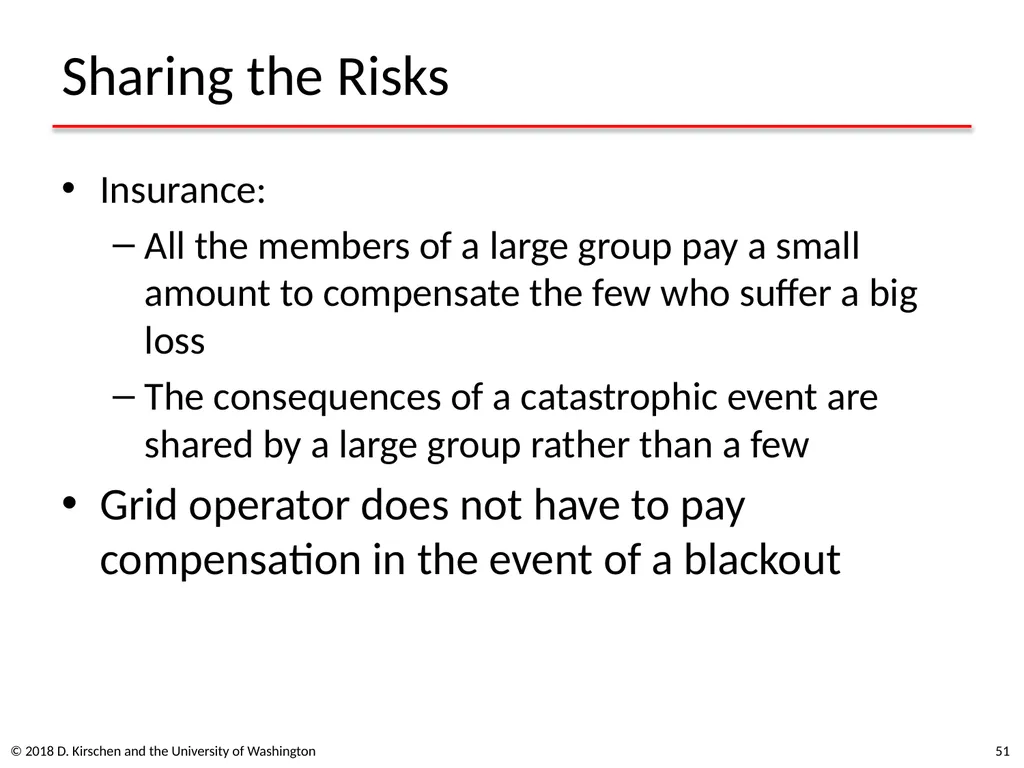
slide51. Sharing the Risks Insurance:
All the members of a large group pay a small amount to compensate the few who suffer a big loss
The consequences of a catastrophic event are shared by a large group rather than a few
Grid operator does not have to pay compensation in the event of a blackout 51 © 2018 D. Kirschen and the University of Washington<br>
slide52. Relocating Risk Possible if one party is more willing or able to accept it
Loss is not catastrophic for this party
This party can offset this loss against gains in other activities
Applies mostly to price risk
How does this relate to markets? 52 © 2018 D. Kirschen and the University of Washington<br>
slide53. Characteristics of markets The time of delivery of the goods
The mode of settlement
Any conditions that might be attached to this transaction © 2018 D. Kirschen and the University of Washington 53<br>
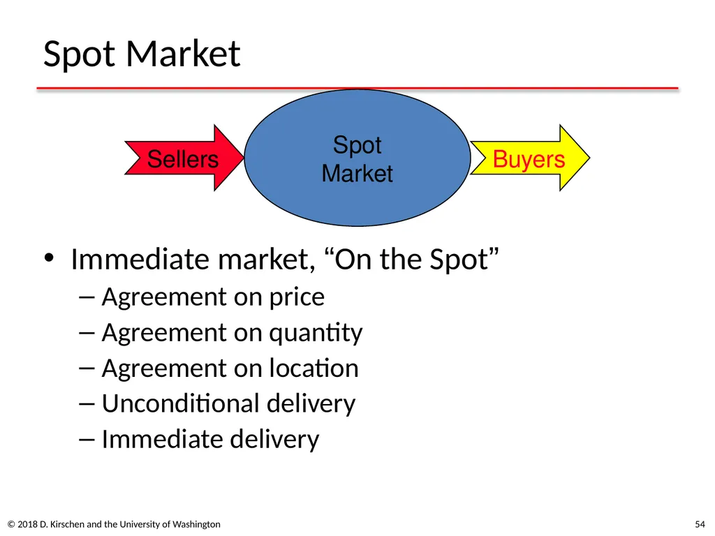
slide54. Spot Market Immediate market, “On the Spot”
Agreement on price
Agreement on quantity
Agreement on location
Unconditional delivery
Immediate delivery 54 Spot
Market Sellers Buyers © 2018 D. Kirschen and the University of Washington<br>
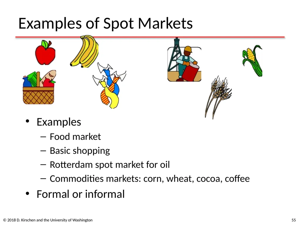
slide55. Examples of Spot Markets Examples
Food market
Basic shopping
Rotterdam spot market for oil
Commodities markets: corn, wheat, cocoa, coffee
Formal or informal 55 © 2018 D. Kirschen and the University of Washington<br>
slide56. Advantages and Disadvantages Advantages:
Simple
Flexible
Immediate
Disadvantages
Prices can fluctuate widely based on circumstances
Example:
Effect of frost in Brazil on the price of coffee beans
Effect of trouble in the Middle East on the price of oil 56 © 2018 D. Kirschen and the University of Washington<br>
slide57. Spot Market Risks Market may not have much depth
Not enough sellers: market is short
Not enough buyers: market is long
Lack of depth causes large price fluctuations
Small producer may have to sell at a low price
Small purchaser may have to buy at a high price
“Price risk”
Relying on the spot market for buying or selling large quantities is a bad idea 57 © 2018 D. Kirschen and the University of Washington<br>
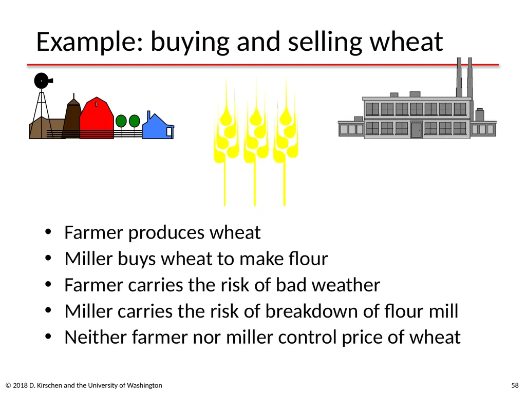
slide58. Example: buying and selling wheat Farmer produces wheat
Miller buys wheat to make flour
Farmer carries the risk of bad weather
Miller carries the risk of breakdown of flour mill
Neither farmer nor miller control price of wheat 58 © 2018 D. Kirschen and the University of Washington<br>
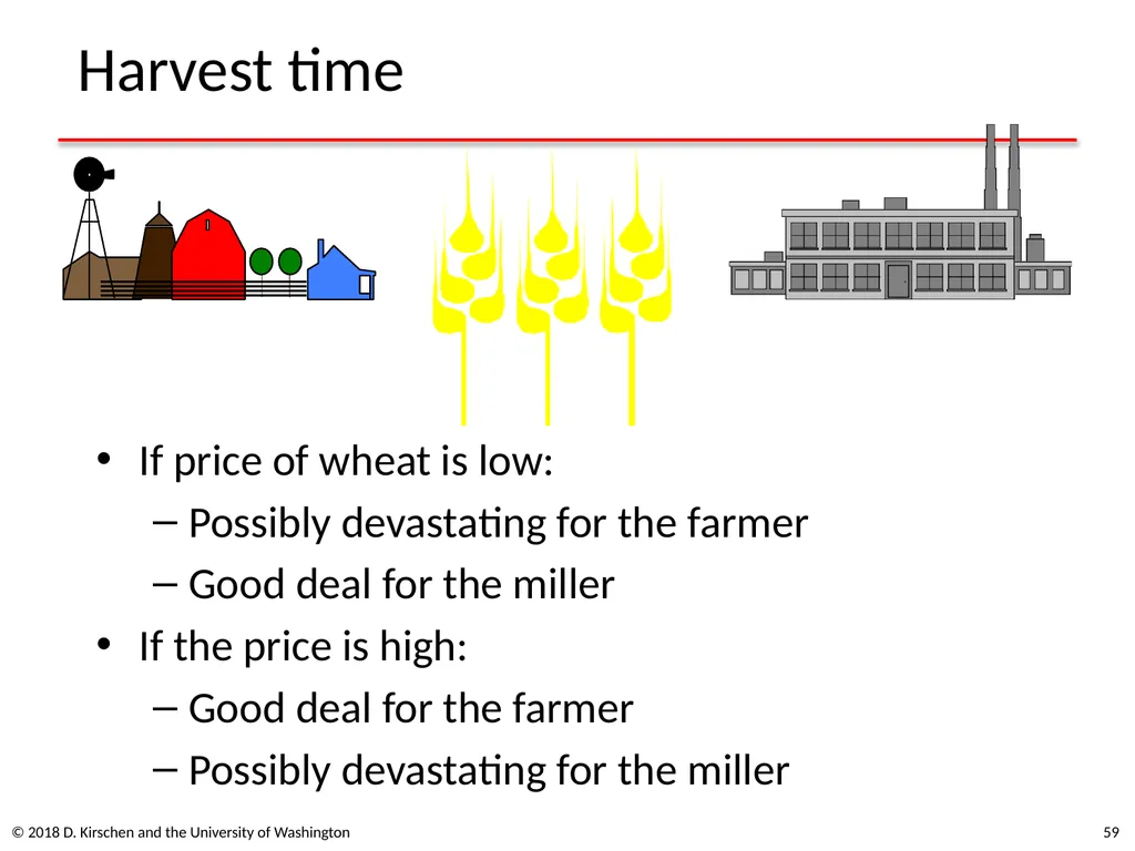
slide59. Harvest time If price of wheat is low:
Possibly devastating for the farmer
Good deal for the miller
If the price is high:
Good deal for the farmer
Possibly devastating for the miller 59 © 2018 D. Kirschen and the University of Washington<br>
slide60. What should they do? Option 1: Accept the spot price of wheat
Equivalent to gambling
Option 2: Agree ahead of time on a price that is acceptable to both parties
Forward contract © 2018 D. Kirschen and the University of Washington 60<br>
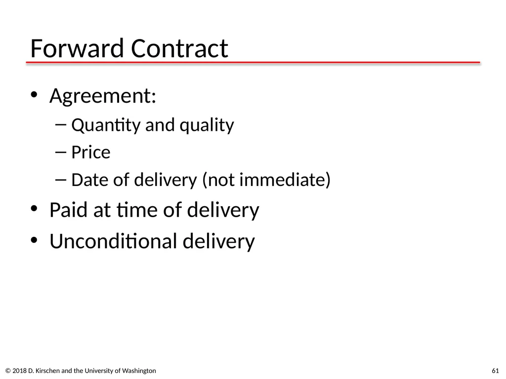
slide61. Forward Contract Agreement:
Quantity and quality
Price
Date of delivery (not immediate)
Paid at time of delivery
Unconditional delivery © 2018 D. Kirschen and the University of Washington 61<br>
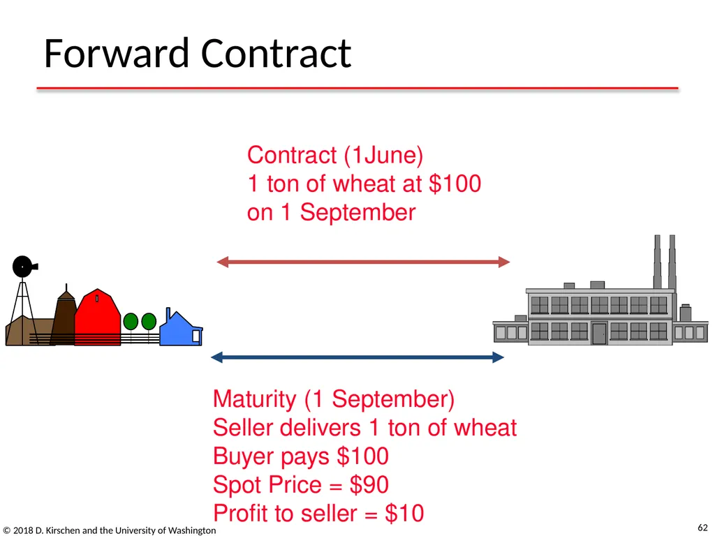
slide62. Forward Contract 62 © 2018 D. Kirschen and the University of Washington<br>
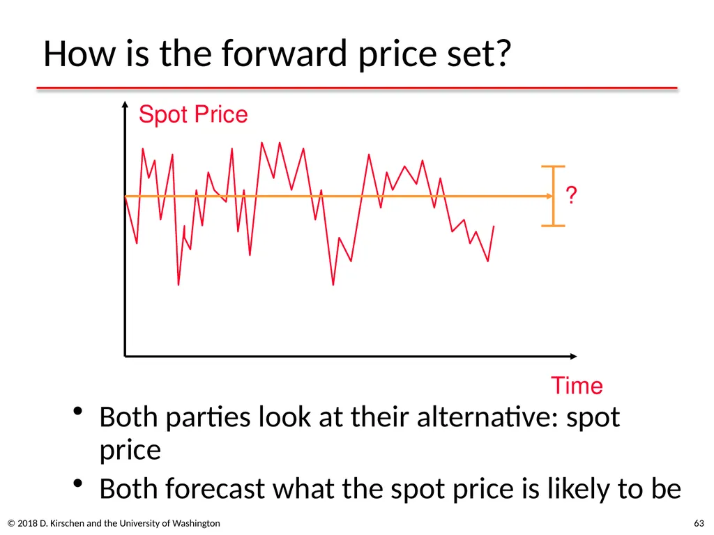
slide63. How is the forward price set? Both parties look at their alternative: spot price
Both forecast what the spot price is likely to be 63 ? © 2018 D. Kirschen and the University of Washington<br>
slide64. Sharing risk In a forward contract, the buyer and seller share the risk that the price differs from their expectation
Difference between contract price and spot price at time of delivery represents a “profit” for one party and a “loss” for the other
However, in the meantime they have been able to get on with their business
Buy new farm machinery
Sell the flour to bakeries 64 © 2018 D. Kirschen and the University of Washington<br>
slide65. Attitudes towards risk Suppose that both parties forecast the same value spot price at time of delivery

Equal attitude towards risk
Forward price is equal to expected spot price

“Risk aversion” 65 © 2018 D. Kirschen and the University of Washington<br>
slide66. Attitudes towards risk If buyer is less risk averse than seller
Buyer can negotiate a forward price lower than the expected spot price
Seller agrees to this lower price because it reduces its risk
Difference between expected spot price and forward price is called a premium
Premium = price that seller is willing to pay to reduce risk 66 © 2018 D. Kirschen and the University of Washington<br>
slide67. Attitudes towards risk If buyer is more risk averse than seller
Seller can negotiate a forward price higher than the expected spot price
Buyer agrees to this higher price because it reduces its risk
Buyer is willing to pay the premium to reduce risk 67 © 2018 D. Kirschen and the University of Washington<br>
slide68. Case 1: Farmer estimates that the spot price will be $100
Miller also forecasts that the spot price will be $100
They can agree on a forward price of $100 68 © 2018 D. Kirschen and the University of Washington<br>
slide69. Case 2: Farmer estimates that the spot price will be $90
Miller forecasts that the spot price will be $110
They can easily agree on a forward price of somewhere between $90 and $110
Exact price will depend on negotiation ability and relative risk aversion 69 © 2018 D. Kirschen and the University of Washington<br>
slide70. Case 3: Farmer estimates that the spot price will be $110
Miller forecasts that the spot price will be $90
Agreeing on a forward price is likely to be difficult unless they have widely different risk aversions 70 © 2018 D. Kirschen and the University of Washington<br>
slide71. Forward Markets Since there are many millers and farmers, a market can be organised for forward contracts
Forward price represents the aggregated expectation of the spot price, plus or minus a risk premium 71 © 2018 D. Kirschen and the University of Washington<br>
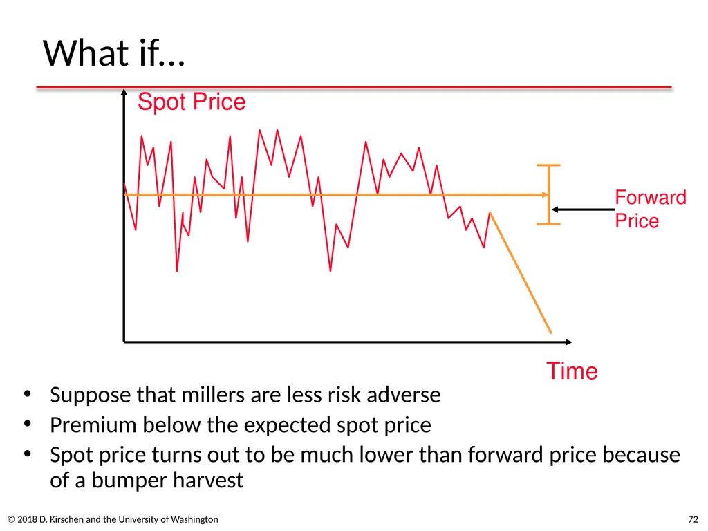
slide72. What if... Suppose that millers are less risk adverse
Premium below the expected spot price
Spot price turns out to be much lower than forward price because of a bumper harvest 72 Forward
Price © 2018 D. Kirschen and the University of Washington<br>
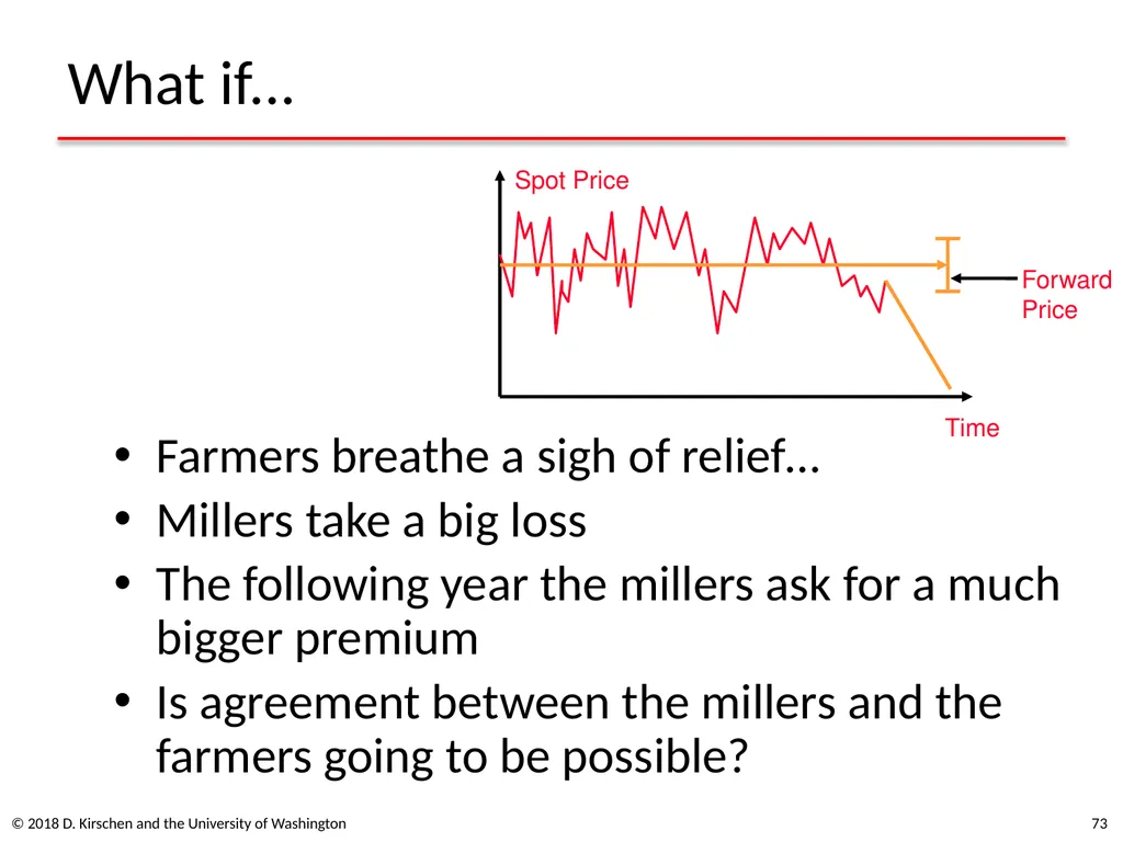
slide73. What if... Farmers breathe a sigh of relief…
Millers take a big loss
The following year the millers ask for a much bigger premium
Is agreement between the millers and the farmers going to be possible? 73 Spot Price Time Forward
Price © 2018 D. Kirschen and the University of Washington<br>
slide74. Undiversified risk Farmers and millers deal only in wheat
Their risk is undiversified
Can only offset “good years” against “bad years”
Risk remains high
Reducing the risk further would help business 74 © 2018 D. Kirschen and the University of Washington<br>
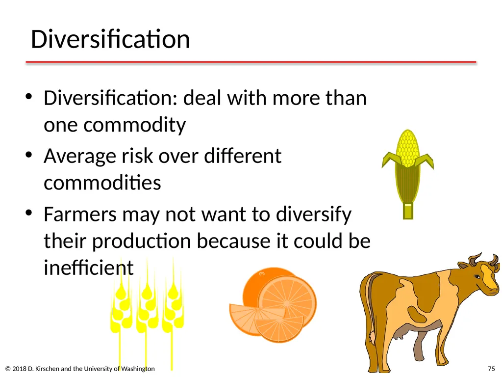
slide75. Diversification Diversification: deal with more than one commodity
Average risk over different commodities
Farmers may not want to diversify their production because it could be inefficient 75 © 2018 D. Kirschen and the University of Washington<br>
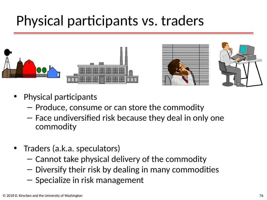
slide76. Physical participants vs. traders Physical participants
Produce, consume or can store the commodity
Face undiversified risk because they deal in only one commodity

Traders (a.k.a. speculators)
Cannot take physical delivery of the commodity
Diversify their risk by dealing in many commodities
Specialize in risk management 76 © 2018 D. Kirschen and the University of Washington<br>
slide77. Trading by speculators Cannot take physical delivery of the commodity
Must balance their position on date of delivery
Quantity bought must equal quantity sold
Buy or sell from spot market if necessary
May involve many transactions
Forward contracts limited to parties who can take physical delivery
Need a standardised contract to reduce the cost of trading: future contract
Future contracts (futures) allow others to participate in the market and share the risk 77 © 2018 D. Kirschen and the University of Washington<br>
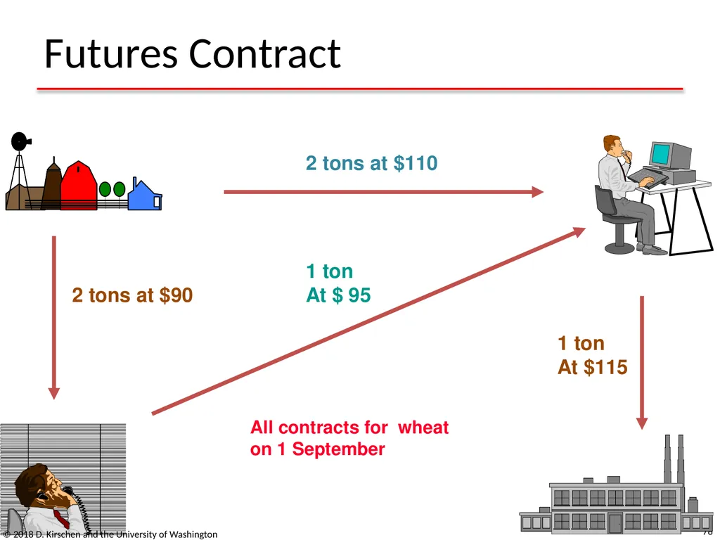
slide78. Futures Contract 78 All contracts for wheat
on 1 September © 2018 D. Kirschen and the University of Washington<br>
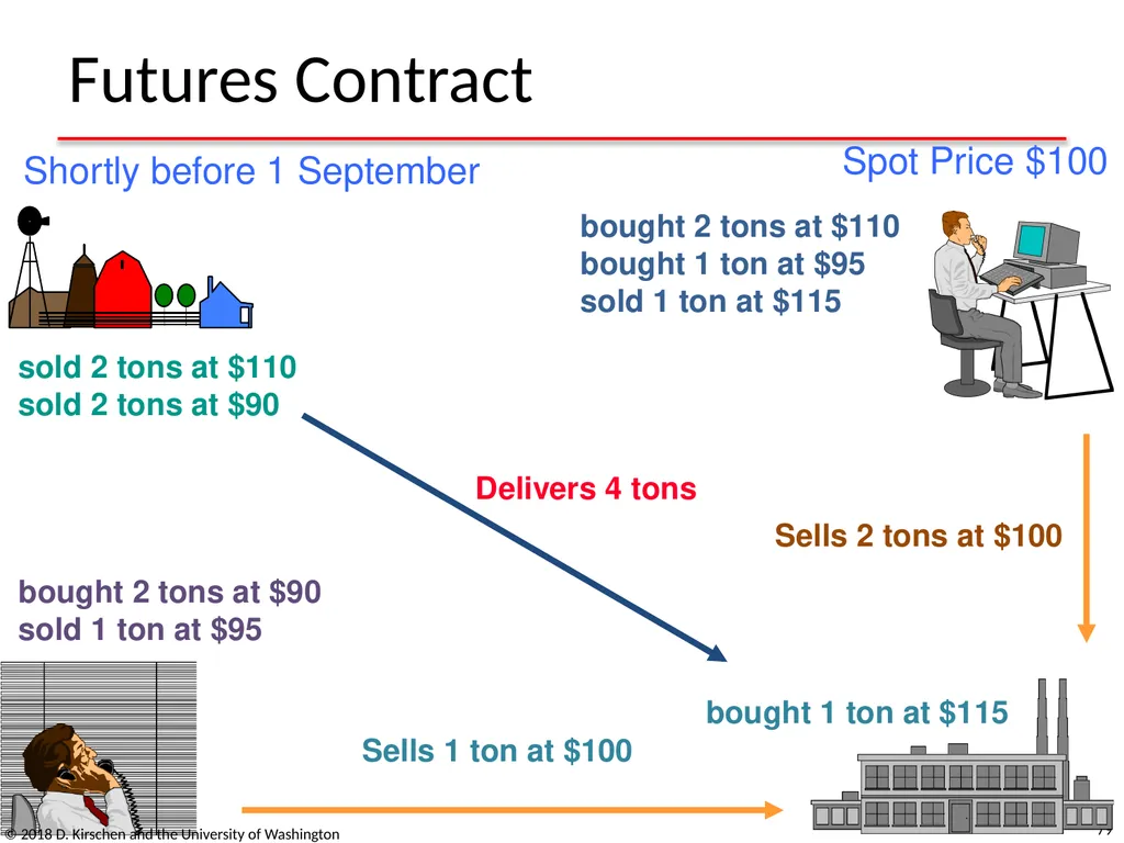
slide79. Futures Contract 79 Shortly before 1 September Spot Price $100 © 2018 D. Kirschen and the University of Washington<br>
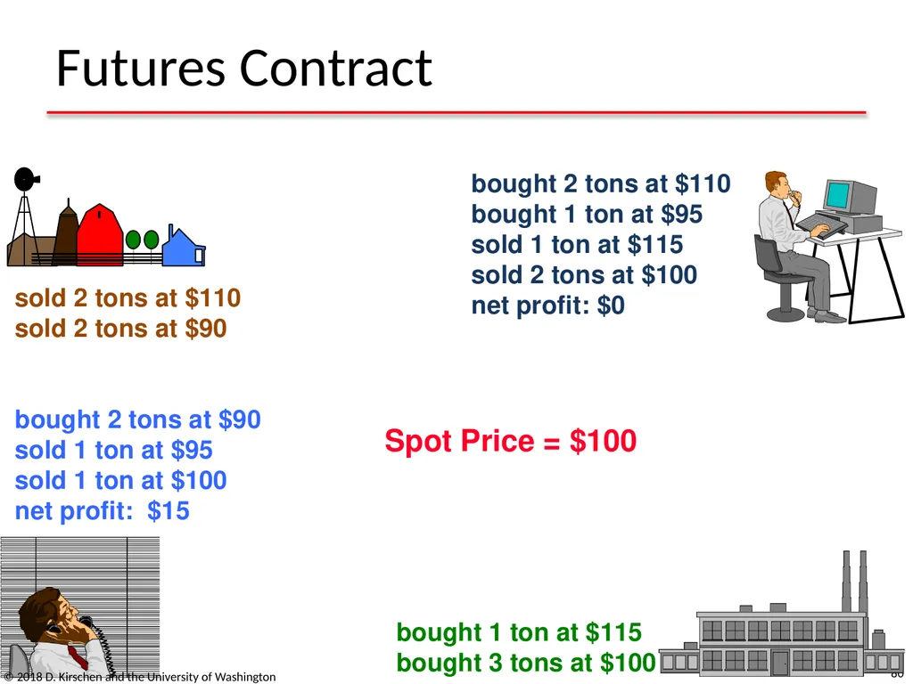
slide80. Futures Contract 80 bought 2 tons at $110
bought 1 ton at $95
sold 1 ton at $115
sold 2 tons at $100
net profit: $0 bought 2 tons at $90
sold 1 ton at $95
sold 1 ton at $100
net profit: $15 bought 1 ton at $115
bought 3 tons at $100 sold 2 tons at $110
sold 2 tons at $90 Spot Price = $100 © 2018 D. Kirschen and the University of Washington<br>
slide81. Importance of information Speculators own some of the commodity before it is delivered
They carry the risk of a price change during that period
Need deep pockets
Without additional information, this is gambling
Information helps speculators make money
Example:
Global perspective on the harvest for wheat
Long term weather forecast and its effect on the demand for gas and electricity © 2018 D. Kirschen and the University of Washington 81<br>
slide82. Options Spot, forward and future contracts: unconditional delivery

Options: conditional delivery
Call Option: right to buy at a certain price at a certain time
Put Option: right to sell at a certain price at a certain time
Two elements of the price:
Exercise or strike price = price paid when option is exercised
Premium or option fee = price paid for the option itself © 2018 D. Kirschen and the University of Washington 82<br>
slide83. Example of Call Option Call Option with an exercise price of $100
About to expire
If the spot market price is $90 the option is worth nothing
If the spot market price is $110 the option is worth $10
Holder makes money if value > option fee © 2018 D. Kirschen and the University of Washington 83<br>
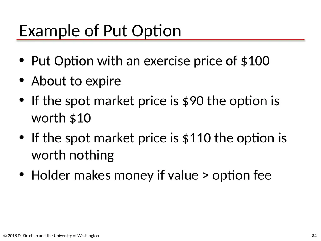
slide84. Example of Put Option Put Option with an exercise price of $100
About to expire
If the spot market price is $90 the option is worth $10
If the spot market price is $110 the option is worth nothing
Holder makes money if value > option fee © 2018 D. Kirschen and the University of Washington 84<br>
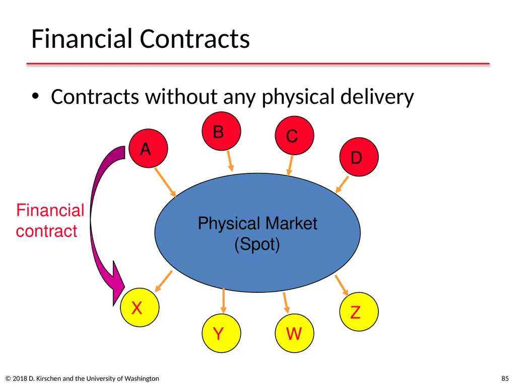
slide85. Financial Contracts Contracts without any physical delivery 85 © 2018 D. Kirschen and the University of Washington<br>
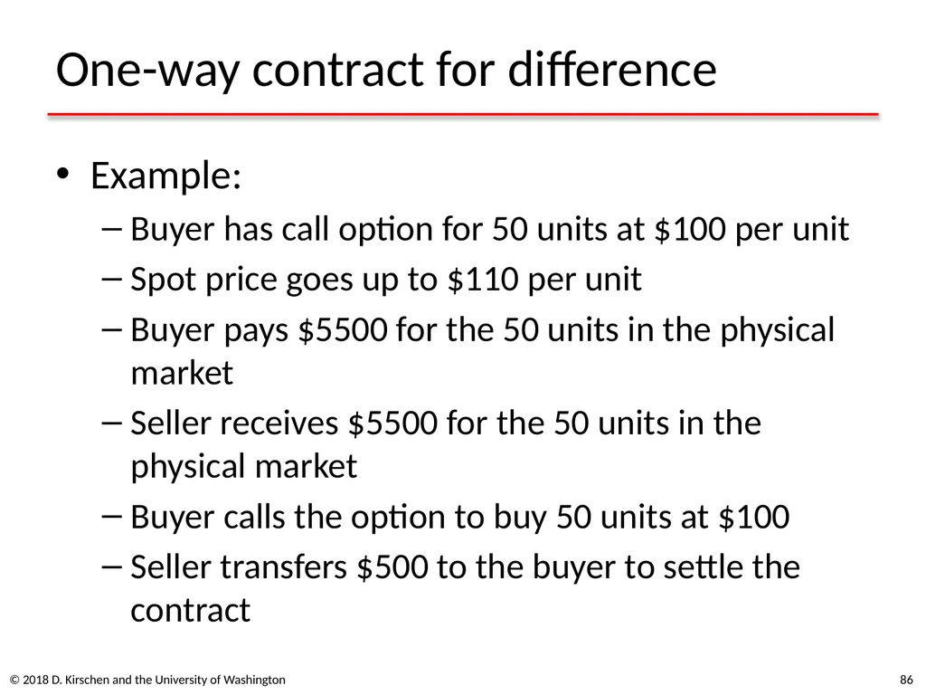
slide86. One-way contract for difference Example:
Buyer has call option for 50 units at $100 per unit
Spot price goes up to $110 per unit
Buyer pays $5500 for the 50 units in the physical market
Seller receives $5500 for the 50 units in the physical market
Buyer calls the option to buy 50 units at $100
Seller transfers $500 to the buyer to settle the contract 86 © 2018 D. Kirschen and the University of Washington<br>
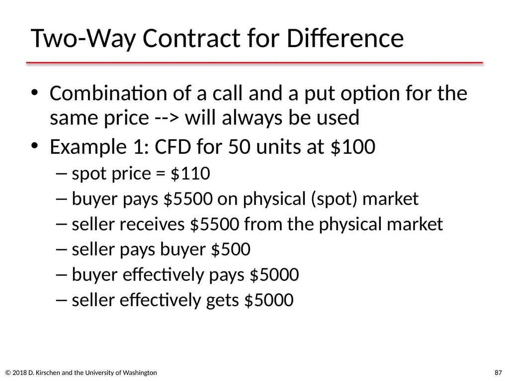
slide87. Two-Way Contract for Difference Combination of a call and a put option for the same price --> will always be used
Example 1: CFD for 50 units at $100
spot price = $110
buyer pays $5500 on physical (spot) market
seller receives $5500 from the physical market
seller pays buyer $500
buyer effectively pays $5000
seller effectively gets $5000 87 © 2018 D. Kirschen and the University of Washington<br>
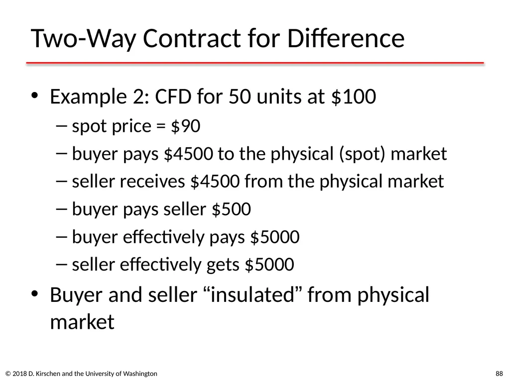
slide88. Two-Way Contract for Difference Example 2: CFD for 50 units at $100
spot price = $90
buyer pays $4500 to the physical (spot) market
seller receives $4500 from the physical market
buyer pays seller $500
buyer effectively pays $5000
seller effectively gets $5000
Buyer and seller “insulated” from physical market 88 © 2018 D. Kirschen and the University of Washington<br>
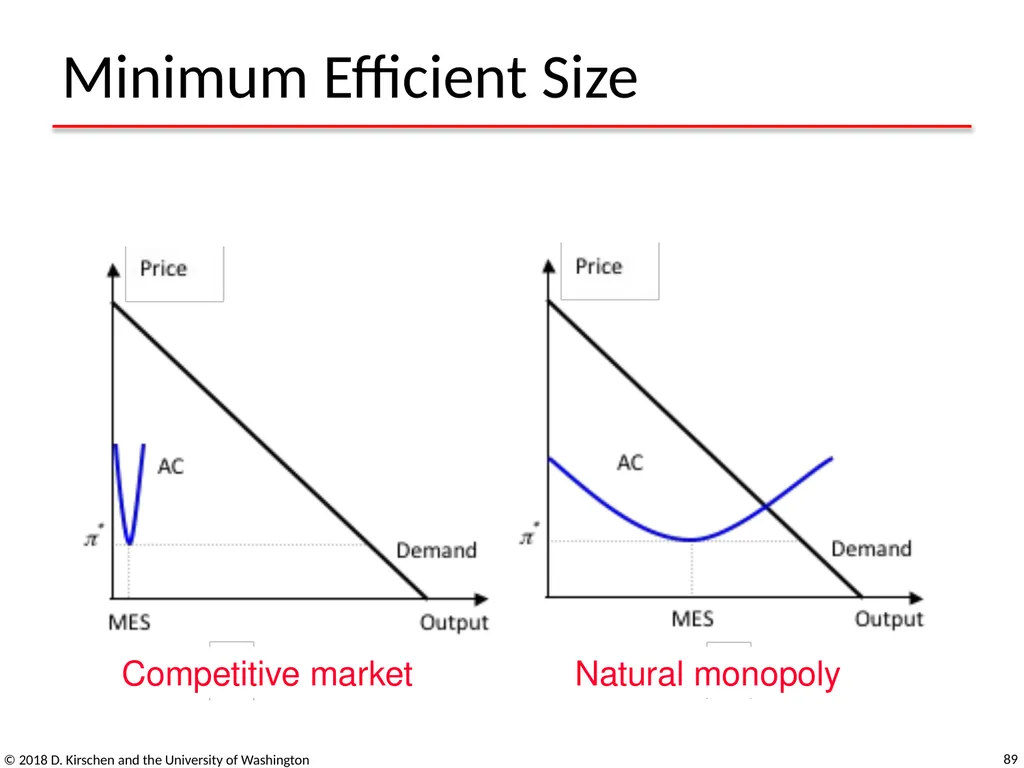
slide89. Minimum Efficient Size © 2018 D. Kirschen and the University of Washington 89 Competitive market Natural monopoly<br>
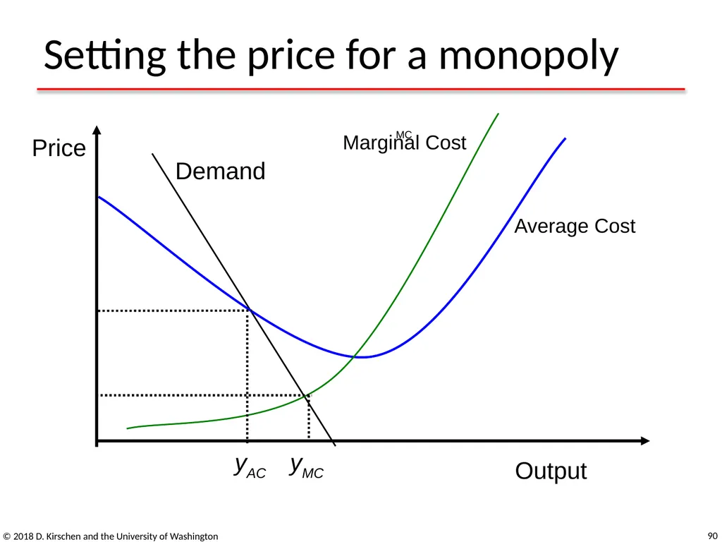
slide90. Setting the price for a monopoly © 2018 D. Kirschen and the University of Washington 90 Price Output Demand MC Average Cost Marginal Cost<br>
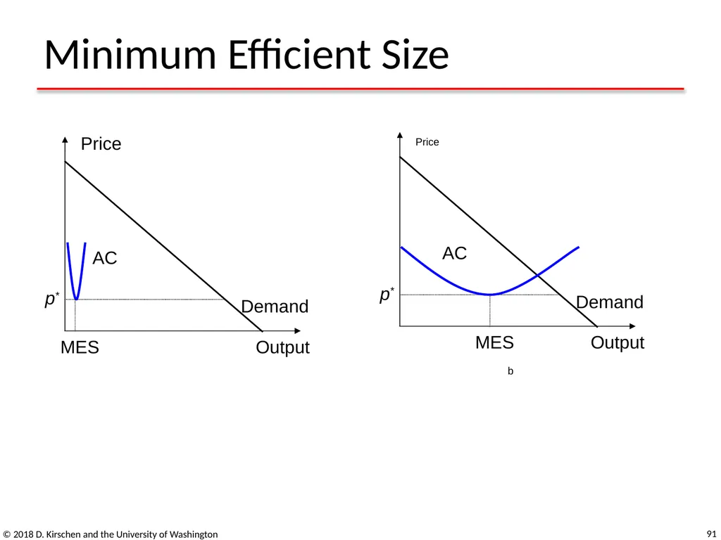
slide91. Minimum Efficient Size © 2018 D. Kirschen and the University of Washington 91<br>
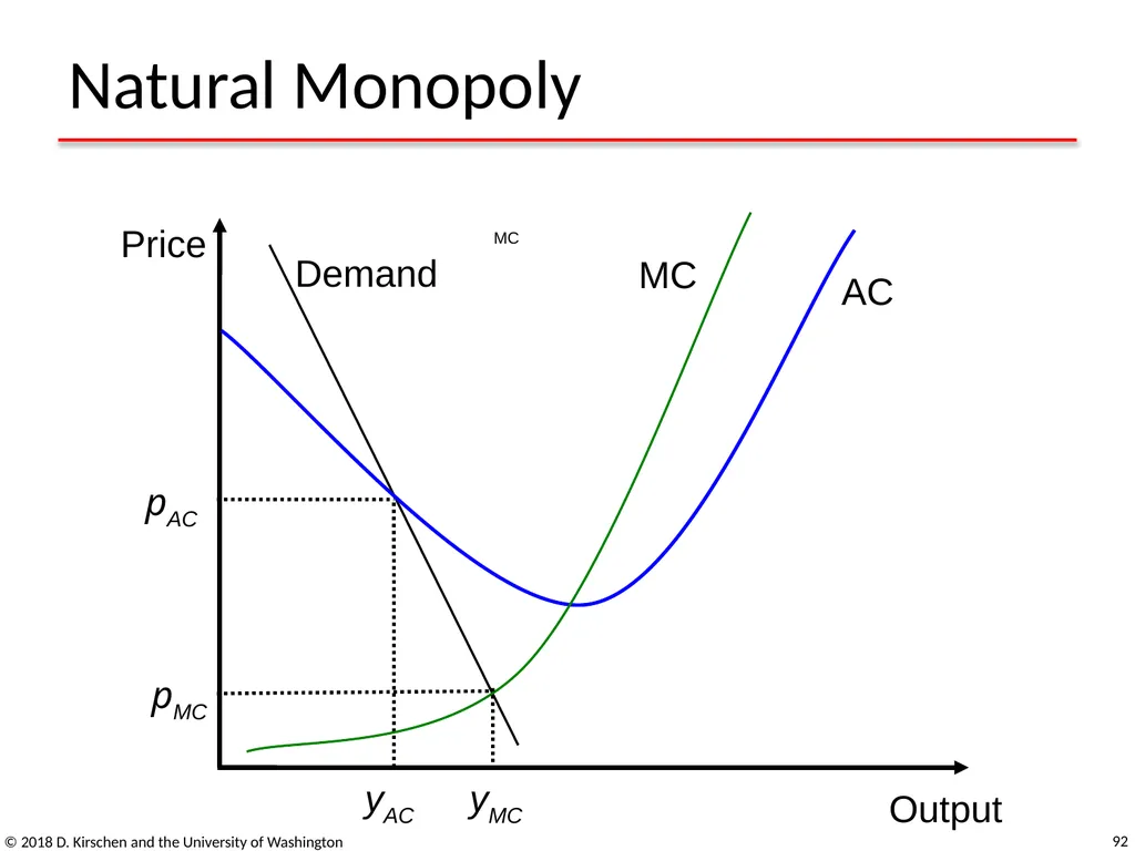
slide92. Natural Monopoly © 2018 D. Kirschen and the University of Washington 92 Price Output Demand yAC pMC MC AC pAC yMC MC<br>