
Chapter 5 – Global Routing 2 Chapter 5 – Global

Description: Chapter 5 Global Routing 2 Chapter 5 Global Routing 5.1 Introduction 5.2 Terminology and Definitions 5.3 Optimization Goals 5.4 Representations of Routing Regions 5.5 The Global Routing Flow 5.6 Single-Net Routing 5.6.1 Rectilinear
Related Topics
Download Presentation
"Chapter 5 – Global Routing 2 Chapter 5 – Global" is the property of its rightful owner. Permission is granted to download and print the materials on this website for personal, non-commercial use only, and to display it on your personal computer provided you do not modify the materials and that you retain all copyright notices contained in the materials. By downloading content from our website, you accept the terms of this agreement.
Presentation Transcript
slide1. Chapter 5 – Global Routing<br>
slide2. 2 Chapter 5 – Global Routing 5.1 Introduction
5.2 Terminology and Definitions
5.3 Optimization Goals
5.4 Representations of Routing Regions
5.5 The Global Routing Flow
5.6 Single-Net Routing
5.6.1 Rectilinear Routing
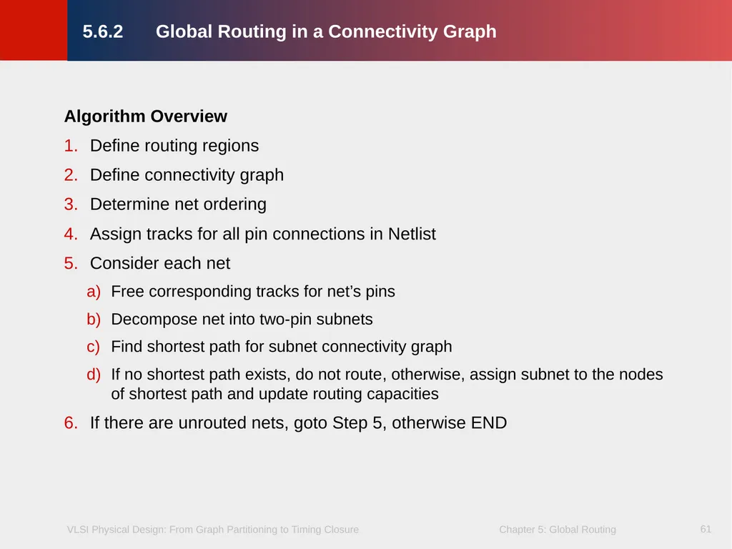
5.6.2 Global Routing in a Connectivity Graph
5.6.3 Finding Shortest Paths with Dijkstra’s Algorithm
5.6.4 Finding Shortest Paths with A* Search
5.7 Full-Netlist Routing
5.7.1 Routing by Integer Linear Programming
5.7.2 Rip-Up and Reroute (RRR)
5.8 Modern Global Routing
5.8.1 Pattern Routing
5.8.2 Negotiated-Congestion Routing<br>
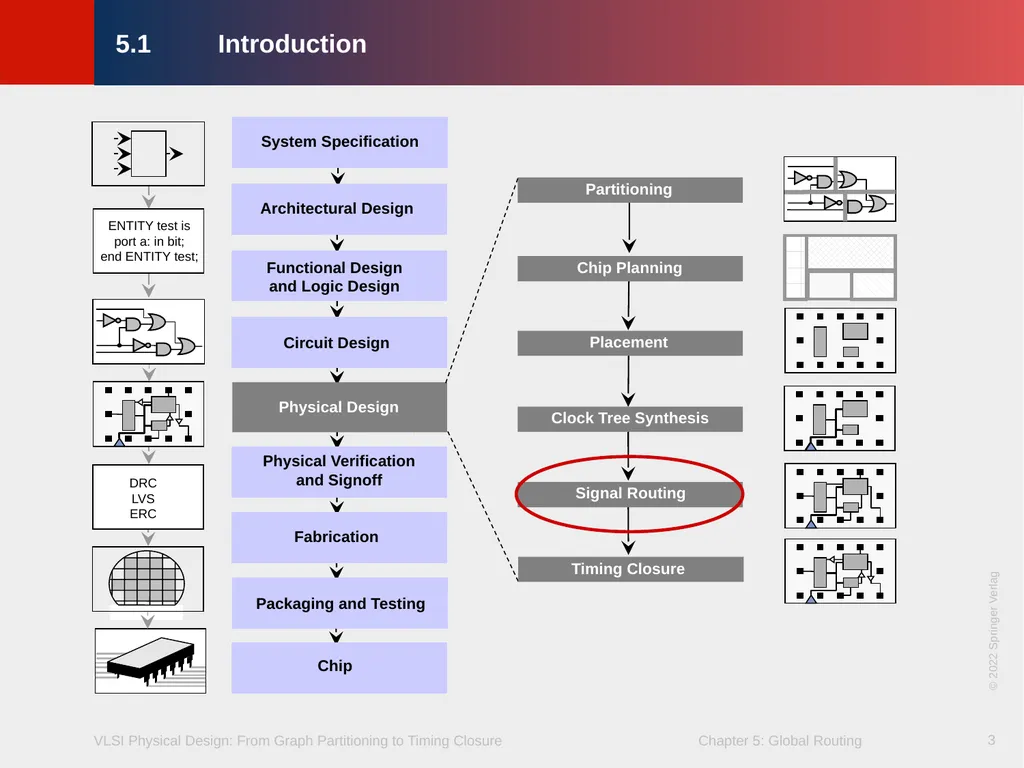
slide3. 3 ENTITY test is port a: in bit; end ENTITY test; DRC LVS
ERC Circuit Design Functional Design and Logic Design Physical Design Physical Verification and Signoff Fabrication System Specification Architectural Design Chip Packaging and Testing Chip Planning Placement Signal Routing Partitioning Timing Closure Clock Tree Synthesis 5.1 Introduction © 2022 Springer Verlag<br>
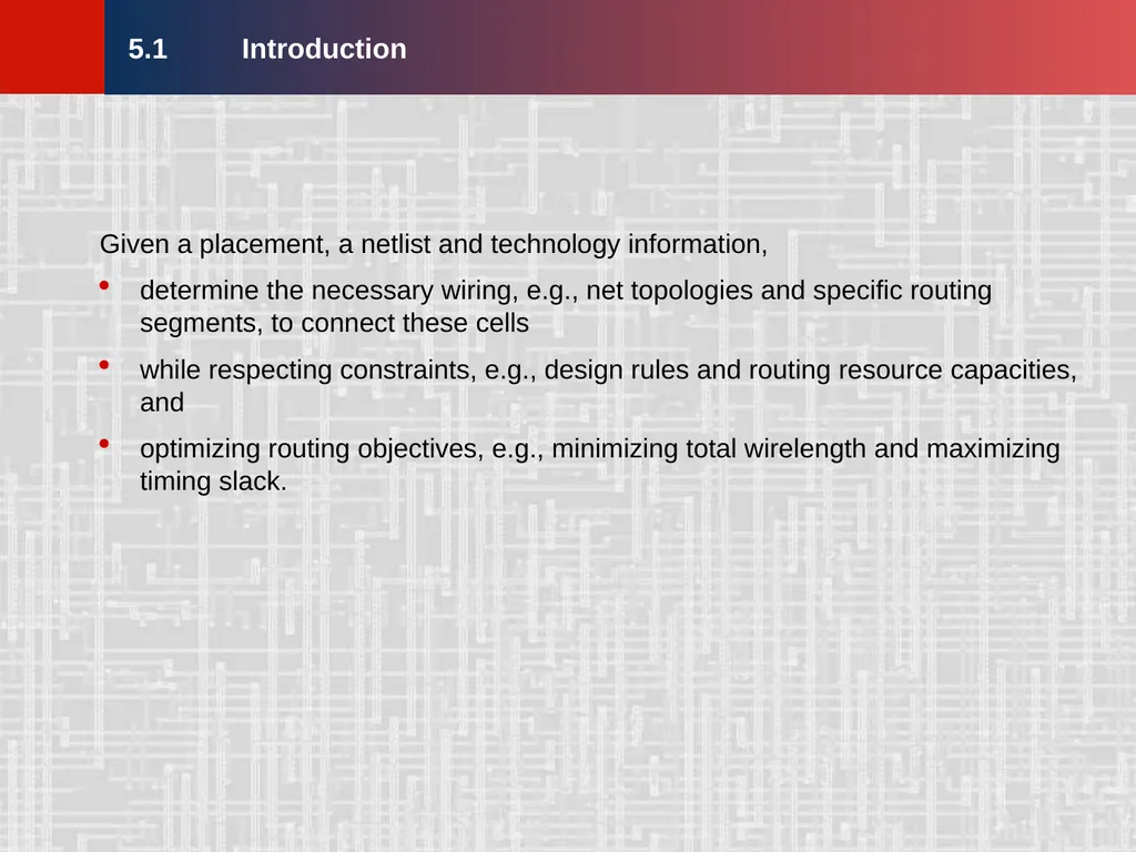
slide4. 4 Given a placement, a netlist and technology information,
determine the necessary wiring, e.g., net topologies and specific routing segments, to connect these cells
while respecting constraints, e.g., design rules and routing resource capacities, and
optimizing routing objectives, e.g., minimizing total wirelength and maximizing timing slack. 5.1 Introduction<br>
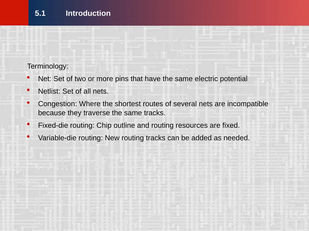
slide5. 5 5 Terminology:
Net: Set of two or more pins that have the same electric potential
Netlist: Set of all nets.
Congestion: Where the shortest routes of several nets are incompatible because they traverse the same tracks.
Fixed-die routing: Chip outline and routing resources are fixed.
Variable-die routing: New routing tracks can be added as needed. 5.1 Introduction<br>
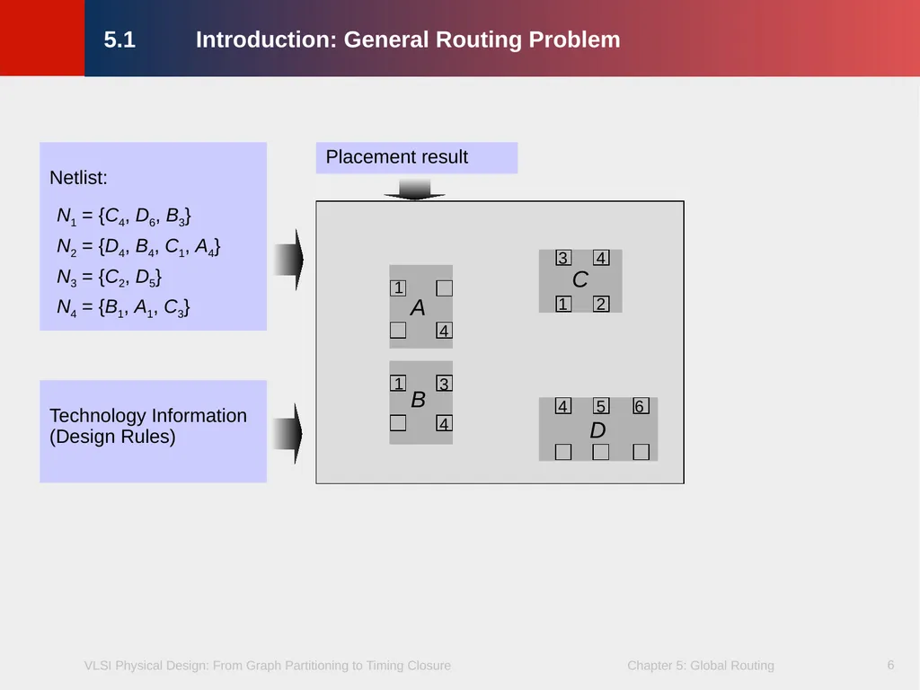
slide6. 6 C D A B 4 3 2 1 4 3 4 1 1 6 5 4 Netlist: N1 = {C4, D6, B3}
N2 = {D4, B4, C1, A4}
N3 = {C2, D5}
N4 = {B1, A1, C3} Technology Information (Design Rules) Placement result 5.1 Introduction: General Routing Problem<br>
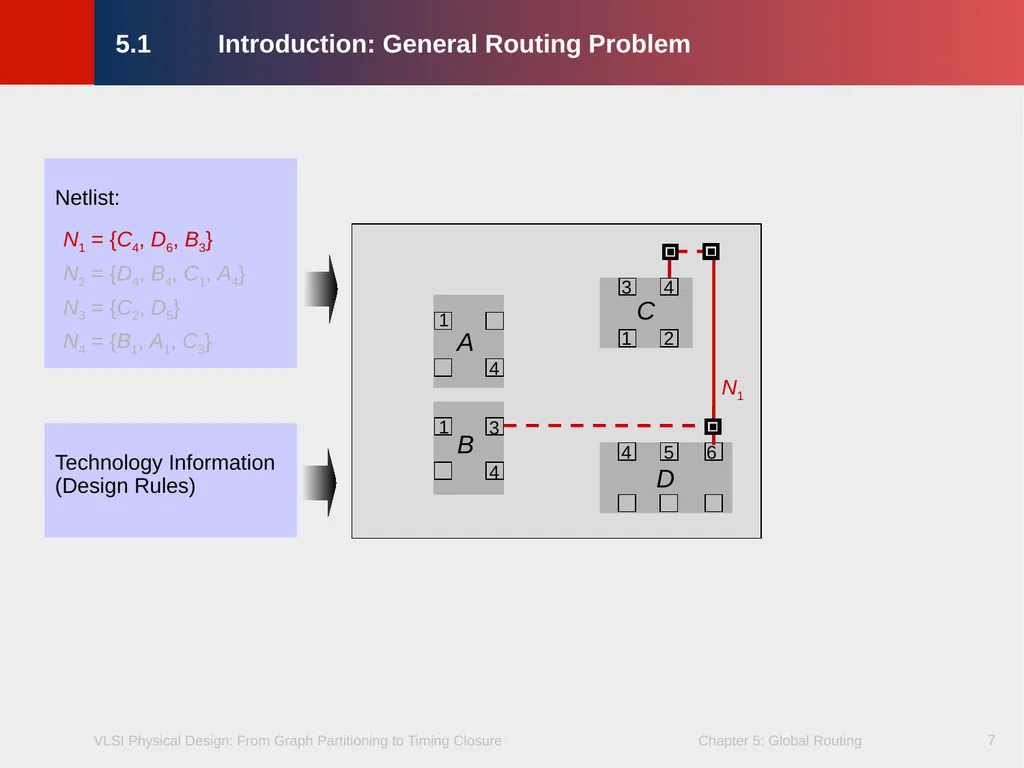
slide7. 7 Netlist: N1 = {C4, D6, B3}
N2 = {D4, B4, C1, A4}
N3 = {C2, D5}
N4 = {B1, A1, C3} Technology Information (Design Rules) 5.1 Introduction: General Routing Problem C D A B 4 3 2 1 4 3 4 1 1 6 5 4 N1<br>
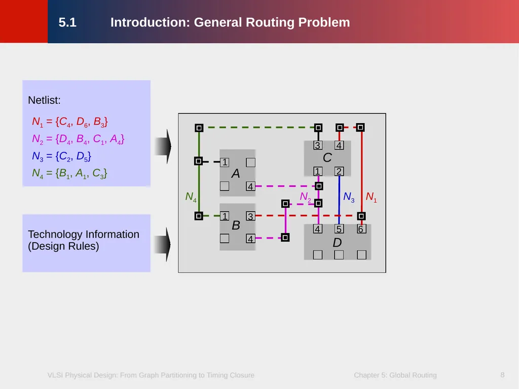
slide8. 8 Netlist: N1 = {C4, D6, B3}
N2 = {D4, B4, C1, A4}
N3 = {C2, D5}
N4 = {B1, A1, C3} Technology Information (Design Rules) 5.1 Introduction: General Routing Problem C D A B 4 3 2 1 4 3 4 1 1 6 5 4 N2 N3 N4 N1<br>
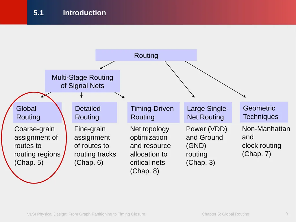
slide9. 9 Timing-Driven Routing Global Routing Detailed
Routing Large Single- Net Routing Coarse-grain assignment of routes to routing regions (Chap. 5) Fine-grain assignment of routes to routing tracks (Chap. 6) Net topology
optimization
and resource
allocation to
critical nets
(Chap. 8) Power (VDD) and Ground (GND)
routing (Chap. 3) Routing Geometric Techniques Non-Manhattan and clock routing
(Chap. 7) 5.1 Introduction Multi-Stage Routing of Signal Nets<br>
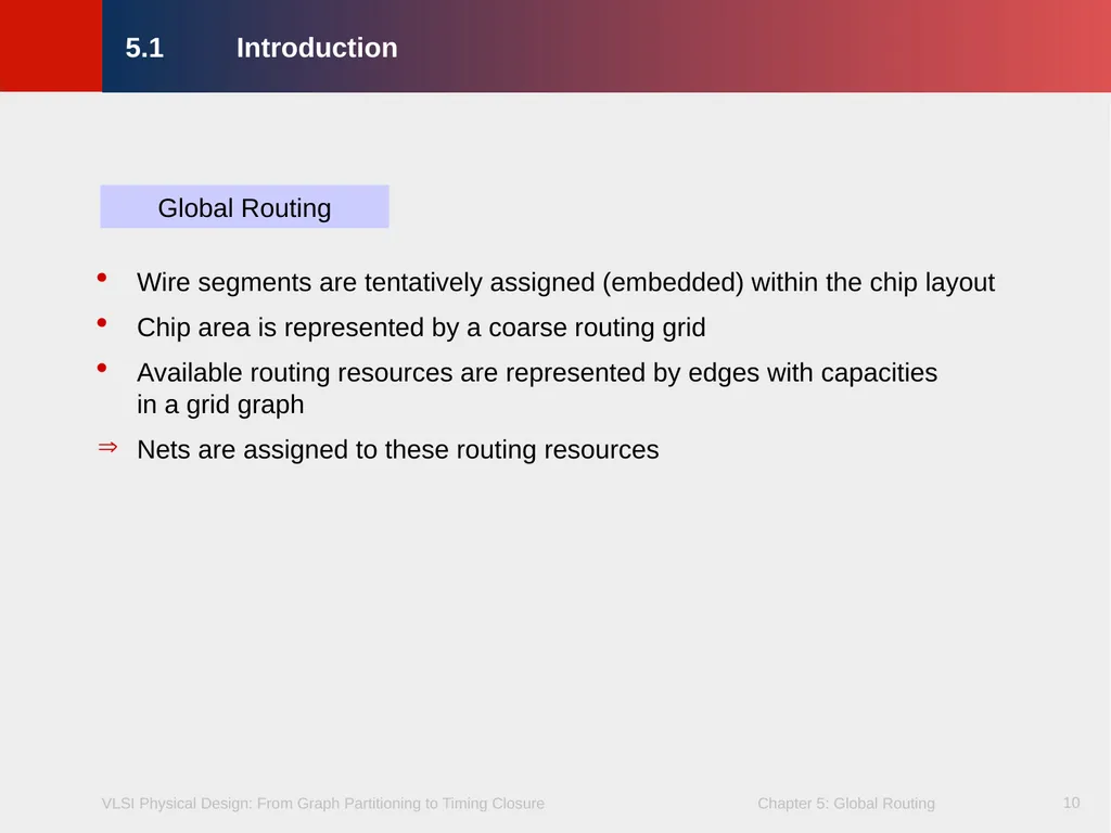
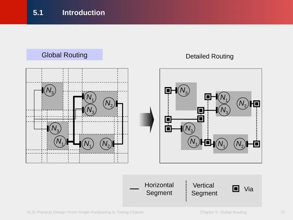
slide10. 10 Wire segments are tentatively assigned (embedded) within the chip layout
Chip area is represented by a coarse routing grid
Available routing resources are represented by edges with capacities in a grid graph
Nets are assigned to these routing resources Global Routing 5.1 Introduction<br>
slide11. 11 Detailed Routing 5.1 Introduction Global Routing<br>
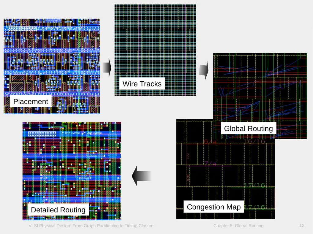
slide12. 12 5.1.2 Globalverdrahtung<br>
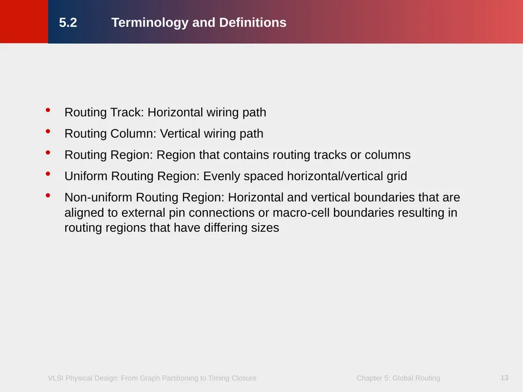
slide13. 13 13 5.2 Terminology and Definitions Routing Track: Horizontal wiring path
Routing Column: Vertical wiring path
Routing Region: Region that contains routing tracks or columns
Uniform Routing Region: Evenly spaced horizontal/vertical grid
Non-uniform Routing Region: Horizontal and vertical boundaries that are aligned to external pin connections or macro-cell boundaries resulting in routing regions that have differing sizes<br>
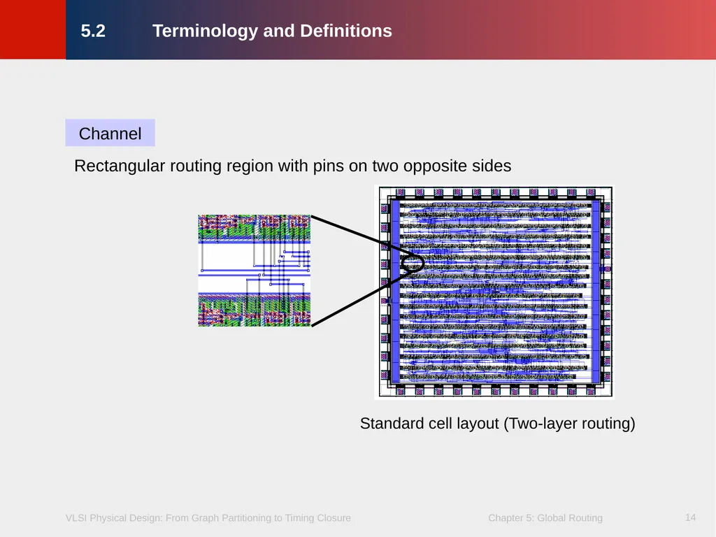
slide14. 14 Channel Standard cell layout (Two-layer routing) 5.2 Terminology and Definitions Rectangular routing region with pins on two opposite sides<br>
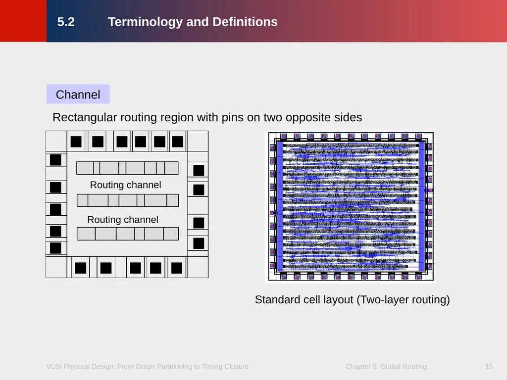
slide15. 15 Routing channel Channel Routing channel 5.2 Terminology and Definitions Standard cell layout (Two-layer routing) Rectangular routing region with pins on two opposite sides<br>
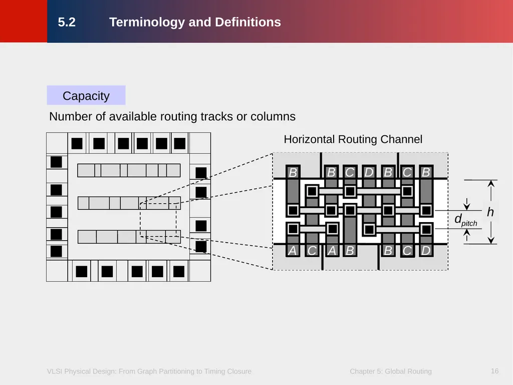
slide16. 16 Capacity 5.2 Terminology and Definitions Number of available routing tracks or columns<br>
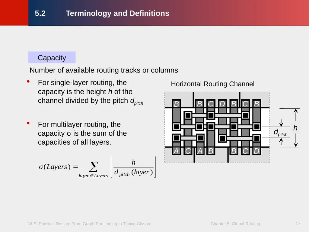
slide17. 17 For single-layer routing, the capacity is the height h of the channel divided by the pitch dpitch
For multilayer routing, the capacity σ is the sum of the capacities of all layers. Capacity A A B B B B B B C C D C C D dpitch h Horizontal Routing Channel 5.2 Terminology and Definitions Number of available routing tracks or columns<br>
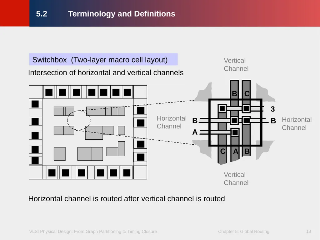
slide18. 18 Horizontal Channel Switchbox (Two-layer macro cell layout) 5.2 Terminology and Definitions Intersection of horizontal and vertical channels Horizontal channel is routed after vertical channel is routed<br>
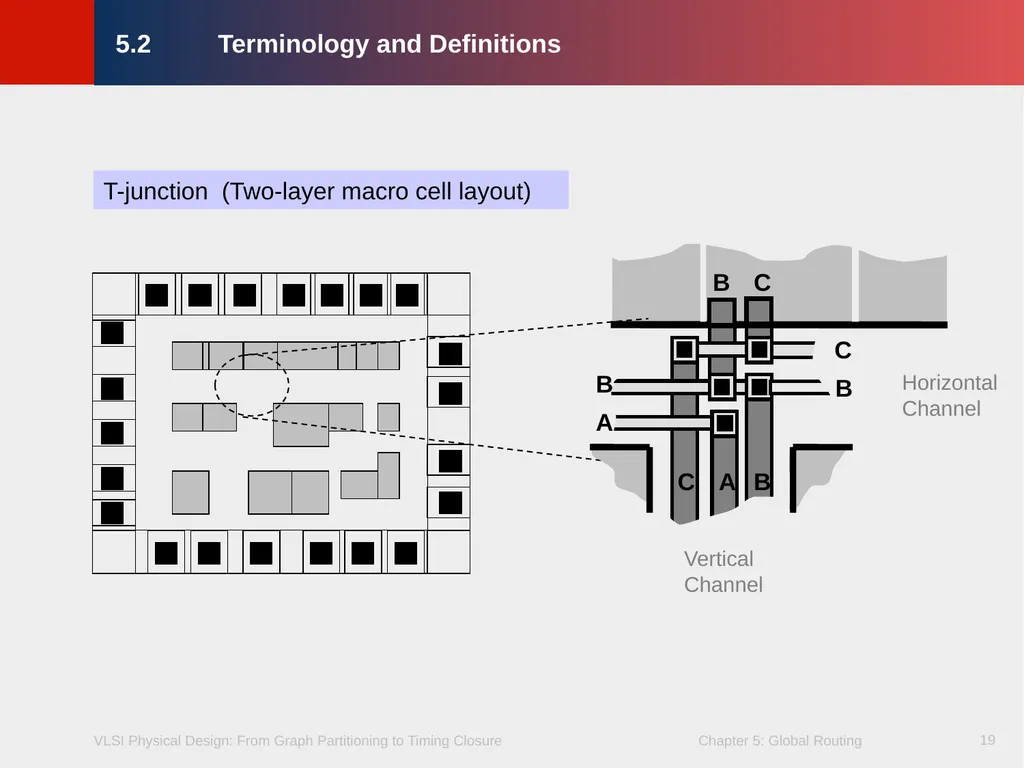
slide19. 19 T-junction (Two-layer macro cell layout) 5.2 Terminology and Definitions<br>
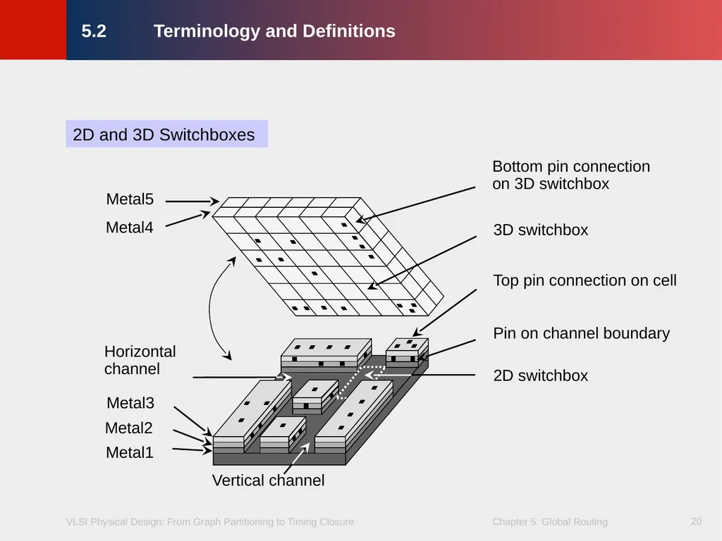
slide20. 20 2D and 3D Switchboxes Metal5 Bottom pin connection on 3D switchbox 3D switchbox 2D switchbox Pin on channel boundary Top pin connection on cell Horizontal channel Metal4 Metal3 Metal2 Metal1 Vertical channel 5.2 Terminology and Definitions<br>
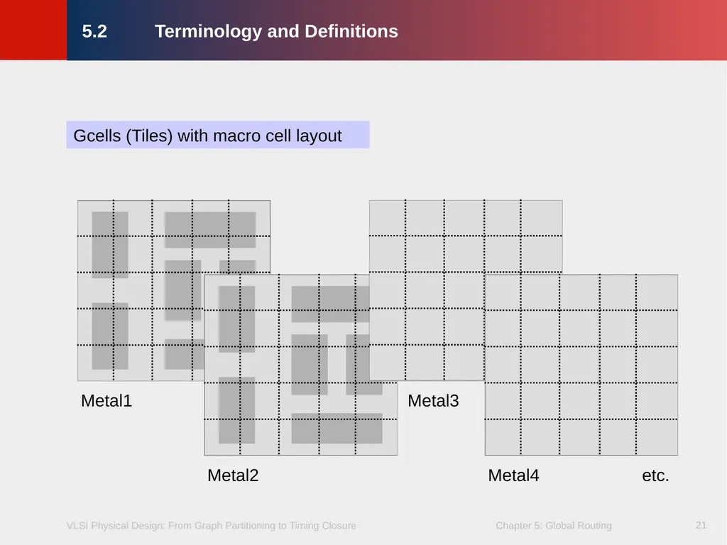
slide21. 21 Gcells (Tiles) with macro cell layout Metal1 etc. 5.2 Terminology and Definitions<br>
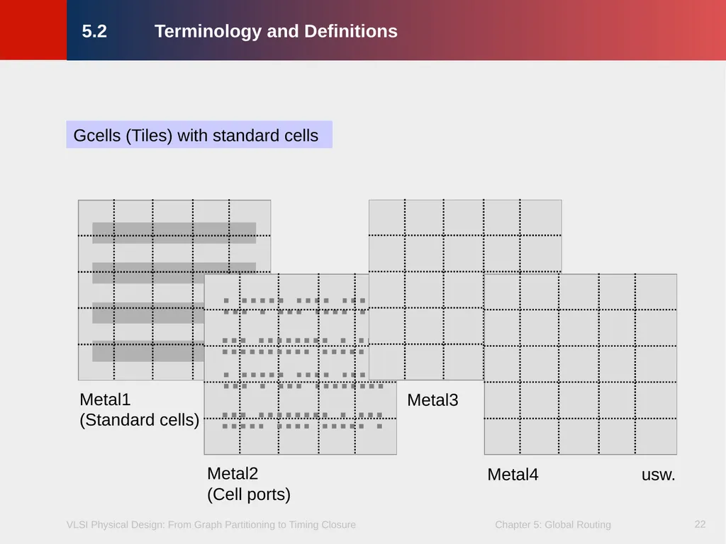
slide22. 22 usw. 5.2 Terminology and Definitions Gcells (Tiles) with standard cells<br>
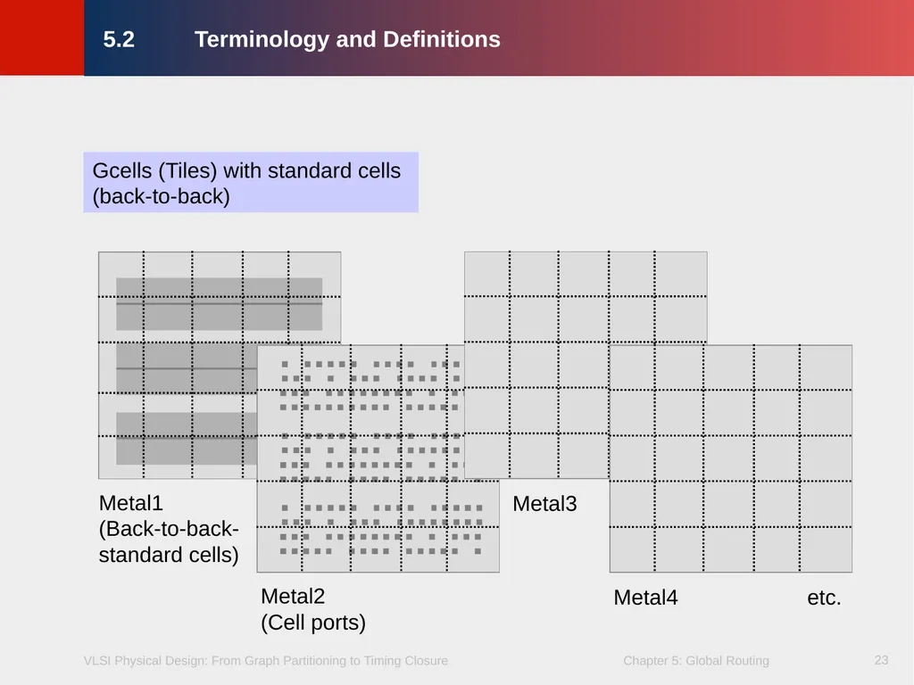
slide23. 23 Metal1 (Back-to-back- standard cells) etc. 5.2 Terminology and Definitions Gcells (Tiles) with standard cells (back-to-back)<br>
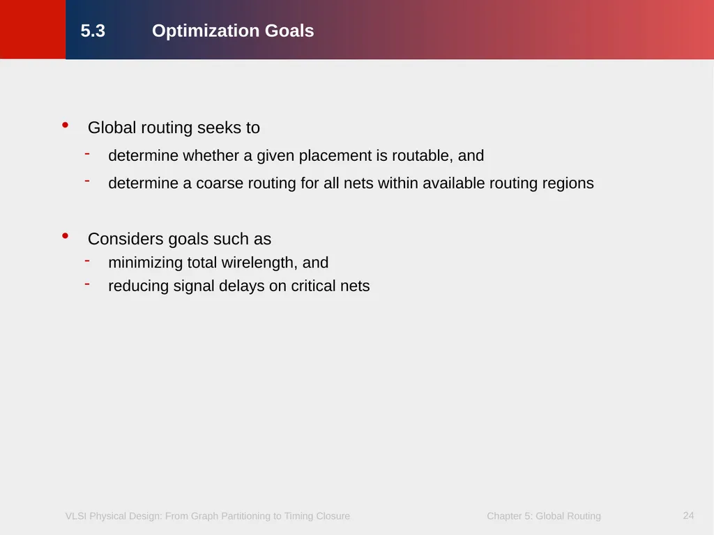
slide24. 24 Global routing seeks to
determine whether a given placement is routable, and
determine a coarse routing for all nets within available routing regions
Considers goals such as
minimizing total wirelength, and
reducing signal delays on critical nets 5.3 Optimization Goals<br>
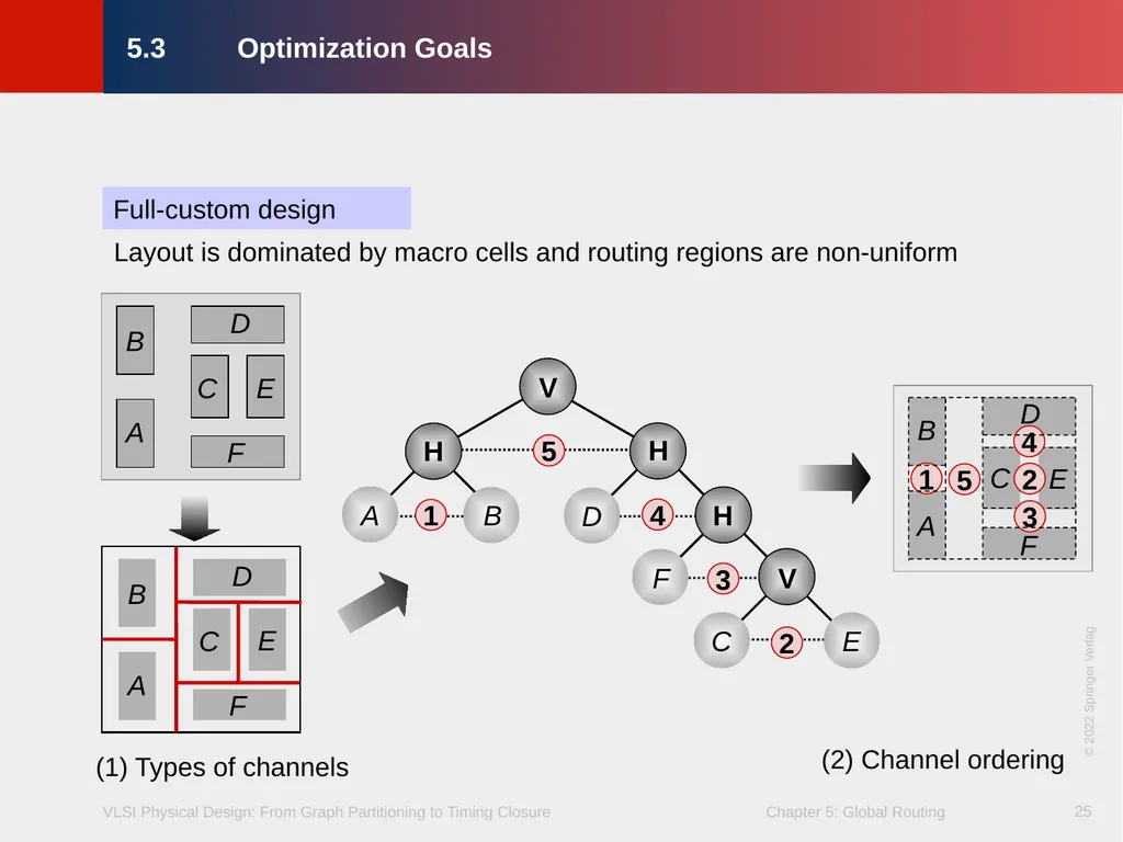
slide25. 25 5.3 Optimization Goals Full-custom design (2) Channel ordering Layout is dominated by macro cells and routing regions are non-uniform © 2022 Springer Verlag<br>
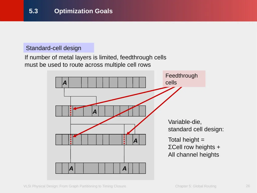
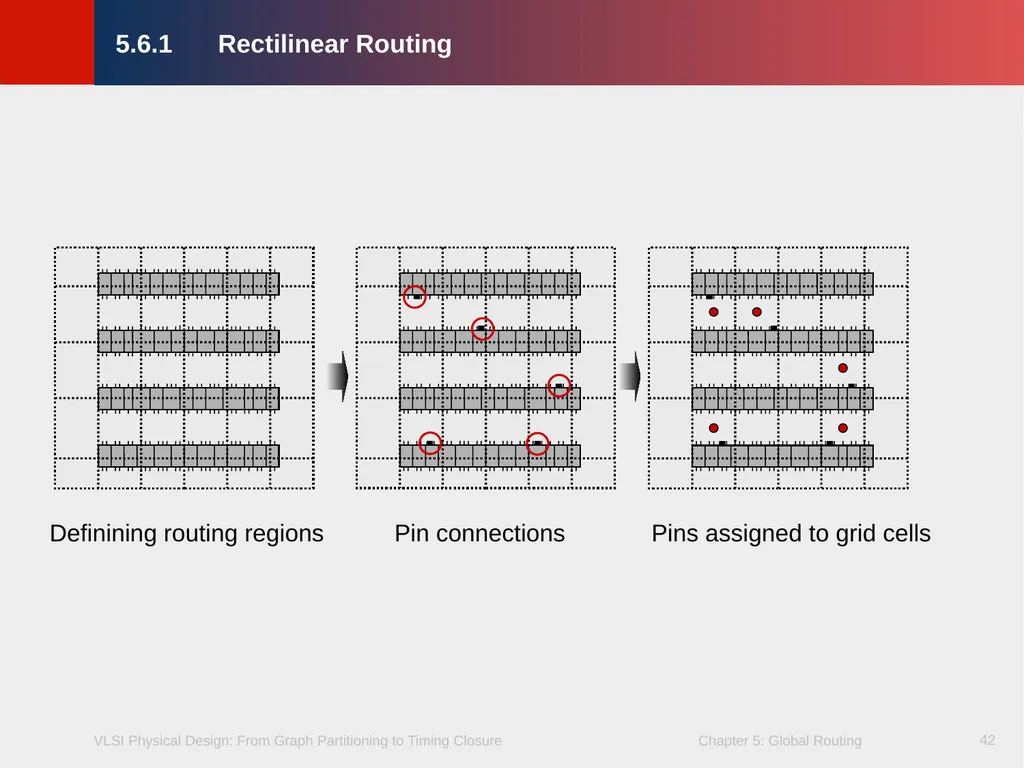
slide26. 26 5.3 Optimization Goals Standard-cell design A A A A A Feedthrough
cells If number of metal layers is limited, feedthrough cells must be used to route across multiple cell rows Variable-die, standard cell design:
Total height = ΣCell row heights + All channel heights<br>
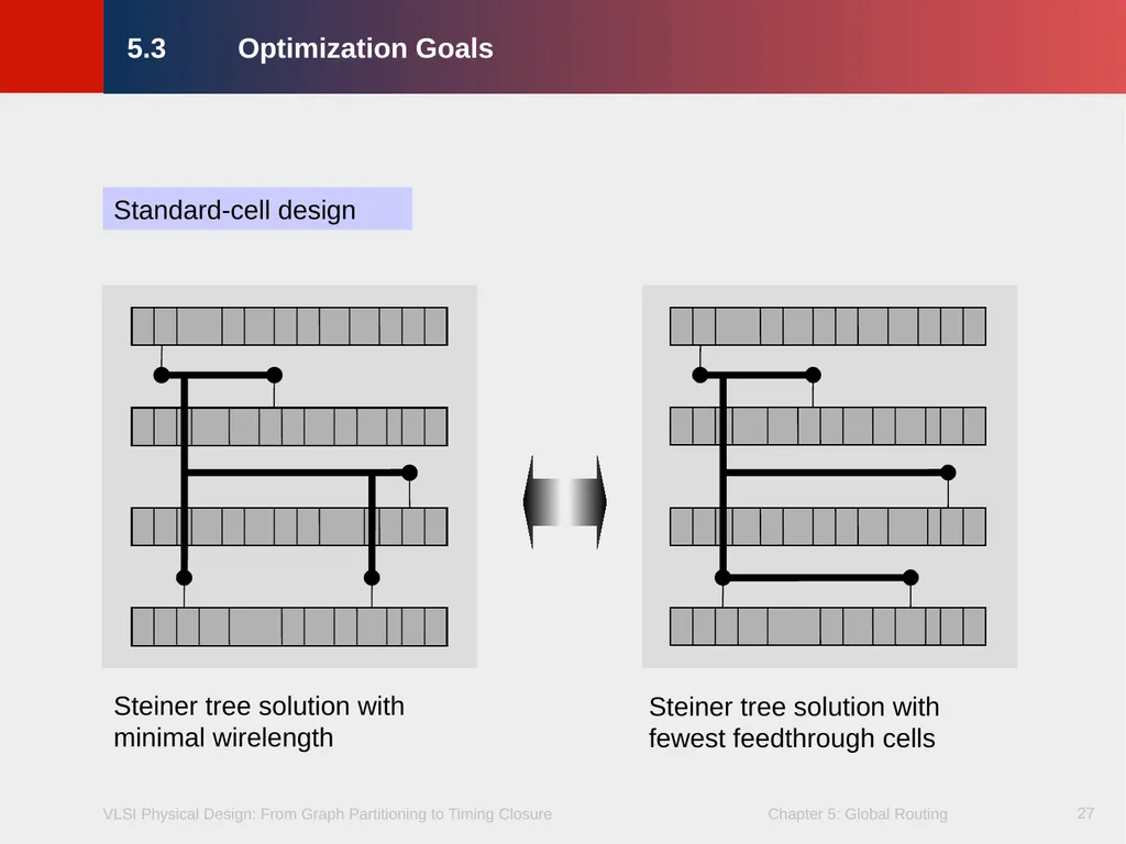
slide27. 27 5.3 Optimization Goals Standard-cell design Steiner tree solution with minimal wirelength Steiner tree solution with
fewest feedthrough cells<br>
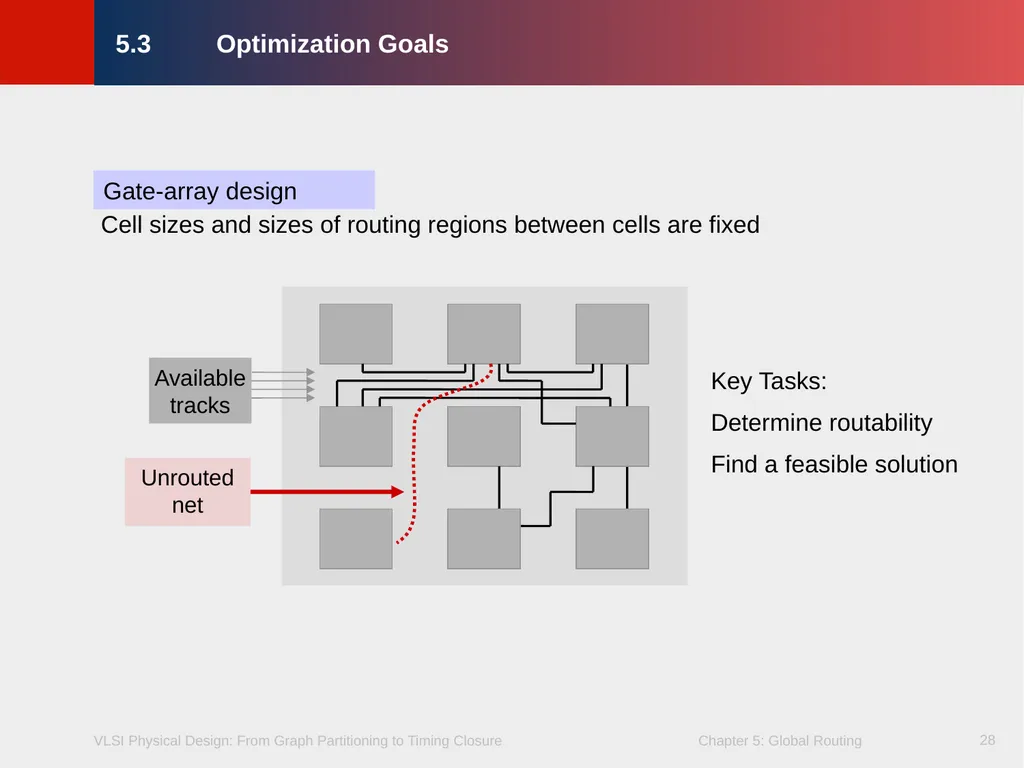
slide28. 28 5.3 Optimization Goals Gate-array design Unrouted net Cell sizes and sizes of routing regions between cells are fixed Key Tasks:
Determine routability
Find a feasible solution<br>
slide29. 29 5.1 Introduction
5.2 Terminology and Definitions
5.3 Optimization Goals
5.4 Representations of Routing Regions
5.5 The Global Routing Flow
5.6 Single-Net Routing
5.6.1 Rectilinear Routing
5.6.2 Global Routing in a Connectivity Graph
5.6.3 Finding Shortest Paths with Dijkstra’s Algorithm
5.6.4 Finding Shortest Paths with A* Search
5.7 Full-Netlist Routing
5.7.1 Routing by Integer Linear Programming
5.7.2 Rip-Up and Reroute (RRR)
5.8 Modern Global Routing
5.8.1 Pattern Routing
5.8.2 Negotiated-Congestion Routing 5.4 Representations of Routing Regions<br>
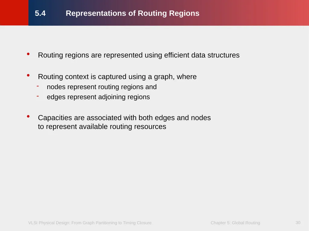
slide30. 30 Routing regions are represented using efficient data structures
Routing context is captured using a graph, where
nodes represent routing regions and
edges represent adjoining regions
Capacities are associated with both edges and nodes to represent available routing resources 5.4 Representations of Routing Regions<br>
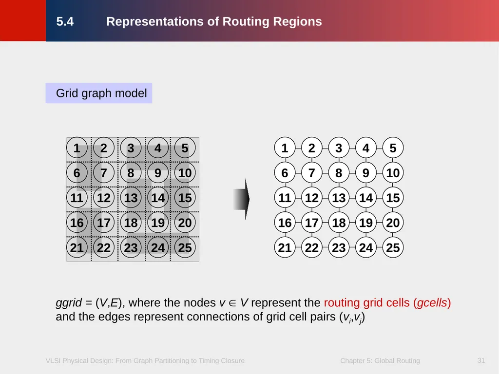
slide31. 31 Grid graph model ggrid = (V,E), where the nodes v V represent the routing grid cells (gcells) and the edges represent connections of grid cell pairs (vi,vj) 5.4 Representations of Routing Regions<br>
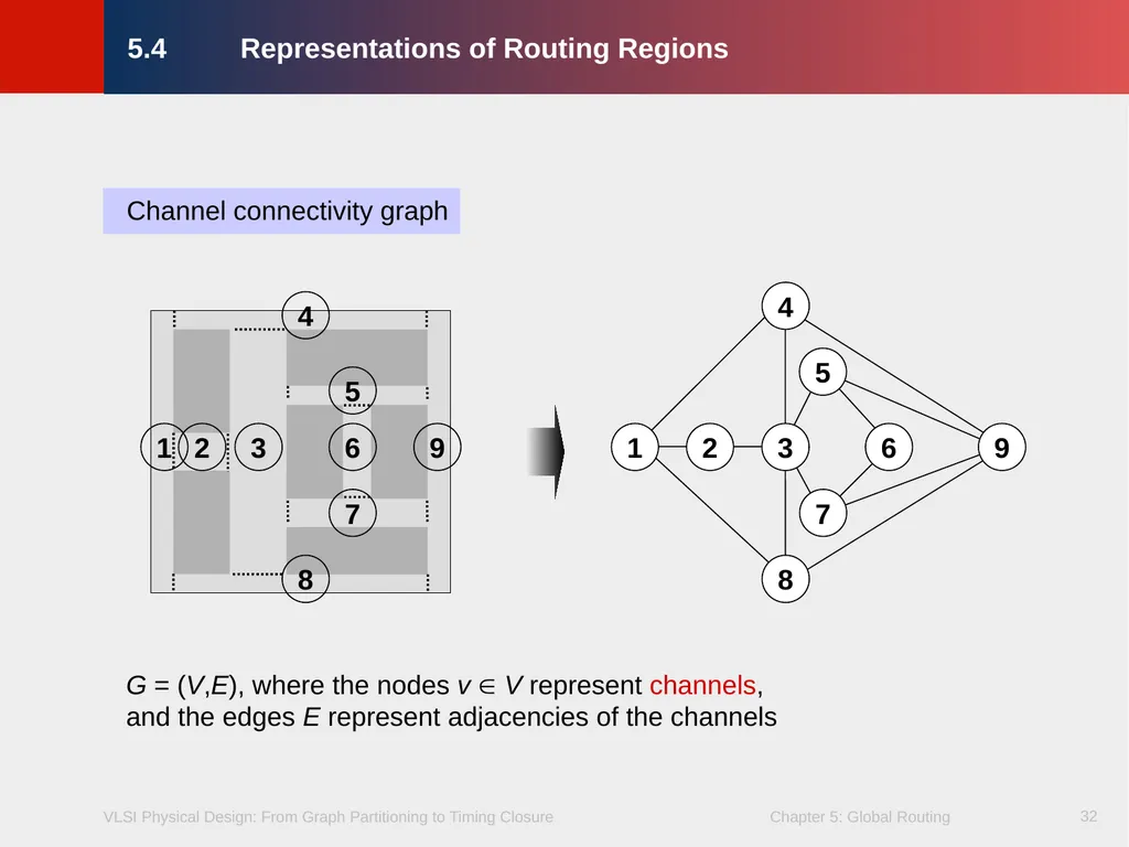
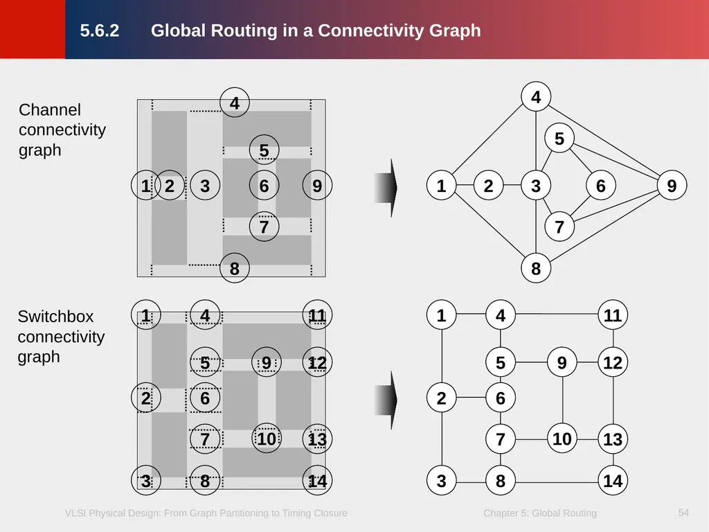
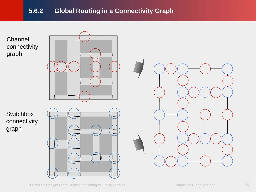
slide32. 32 Channel connectivity graph G = (V,E), where the nodes v V represent channels, and the edges E represent adjacencies of the channels 5.4 Representations of Routing Regions<br>
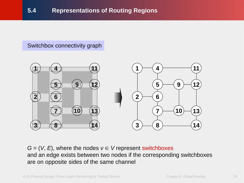
slide33. 33 Switchbox connectivity graph G = (V, E), where the nodes v V represent switchboxes and an edge exists between two nodes if the corresponding switchboxes are on opposite sides of the same channel 5.4 Representations of Routing Regions<br>
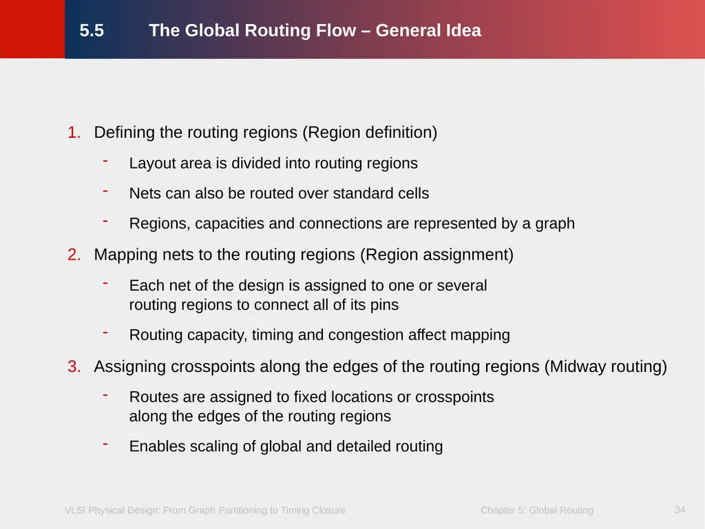
slide34. 34 5.5 The Global Routing Flow – General Idea Defining the routing regions (Region definition)
Layout area is divided into routing regions
Nets can also be routed over standard cells
Regions, capacities and connections are represented by a graph
Mapping nets to the routing regions (Region assignment)
Each net of the design is assigned to one or several routing regions to connect all of its pins
Routing capacity, timing and congestion affect mapping
Assigning crosspoints along the edges of the routing regions (Midway routing)
Routes are assigned to fixed locations or crosspoints along the edges of the routing regions
Enables scaling of global and detailed routing<br>
slide35. 35 5.1 Introduction
5.2 Terminology and Definitions
5.3 Optimization Goals
5.4 Representations of Routing Regions
5.5 The Global Routing Flow
5.6 Single-Net Routing
5.6.1 Rectilinear Routing
5.6.2 Global Routing in a Connectivity Graph
5.6.3 Finding Shortest Paths with Dijkstra’s Algorithm
5.6.4 Finding Shortest Paths with A* Search
5.7 Full-Netlist Routing
5.7.1 Routing by Integer Linear Programming
5.7.2 Rip-Up and Reroute (RRR)
5.8 Modern Global Routing
5.8.1 Pattern Routing
5.8.2 Negotiated-Congestion Routing 5.6 Single-Net Routing<br>
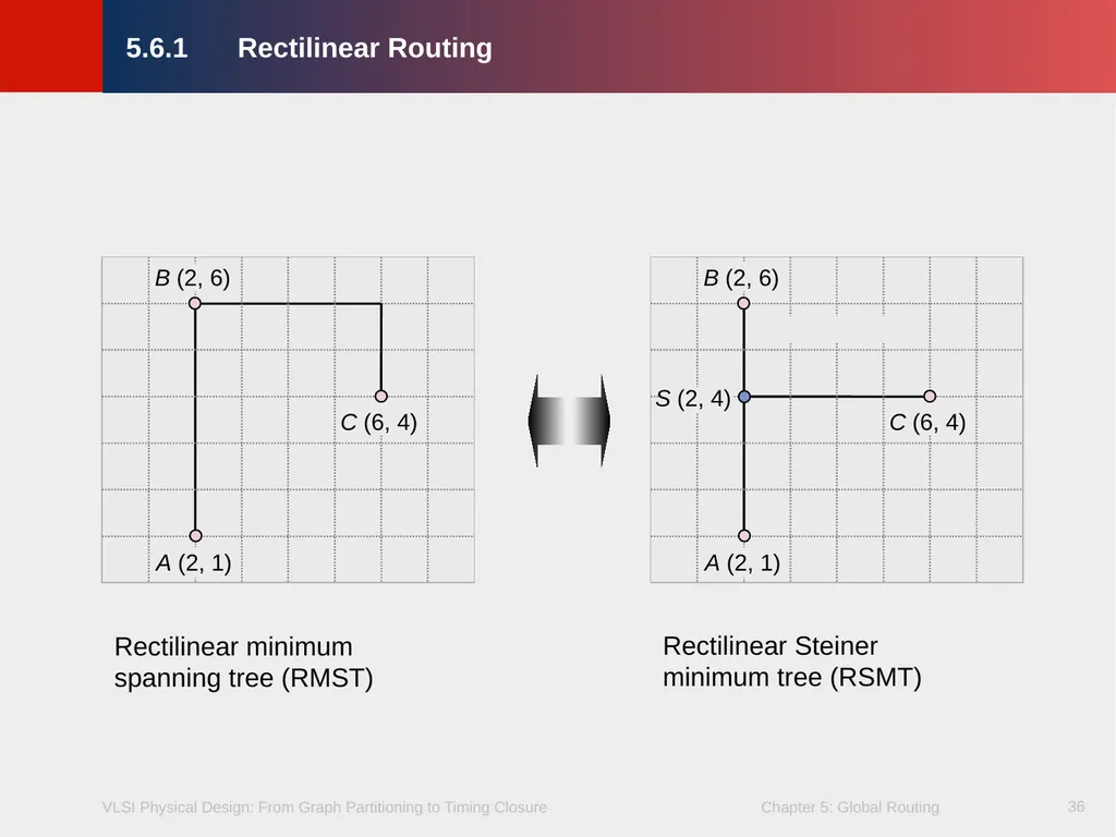
slide36. 36 B (2, 6) A (2, 1) C (6, 4) B (2, 6) A (2, 1) C (6, 4) S (2, 4) Rectilinear Steiner minimum tree (RSMT) Rectilinear minimum spanning tree (RMST) 5.6.1 Rectilinear Routing<br>
slide37. 37 37 5.6.1 Rectilinear Routing An RMST can be computed in O(p2) time, where p is the number of terminals in the net using methods such as Prim’s Algorithm
Prim’s Algorithm builds an MST by starting with a single terminal and greedily adding least-cost edges to the partially-constructed tree
Advanced computational-geometric techniques reduce the runtime to O(p log p)<br>
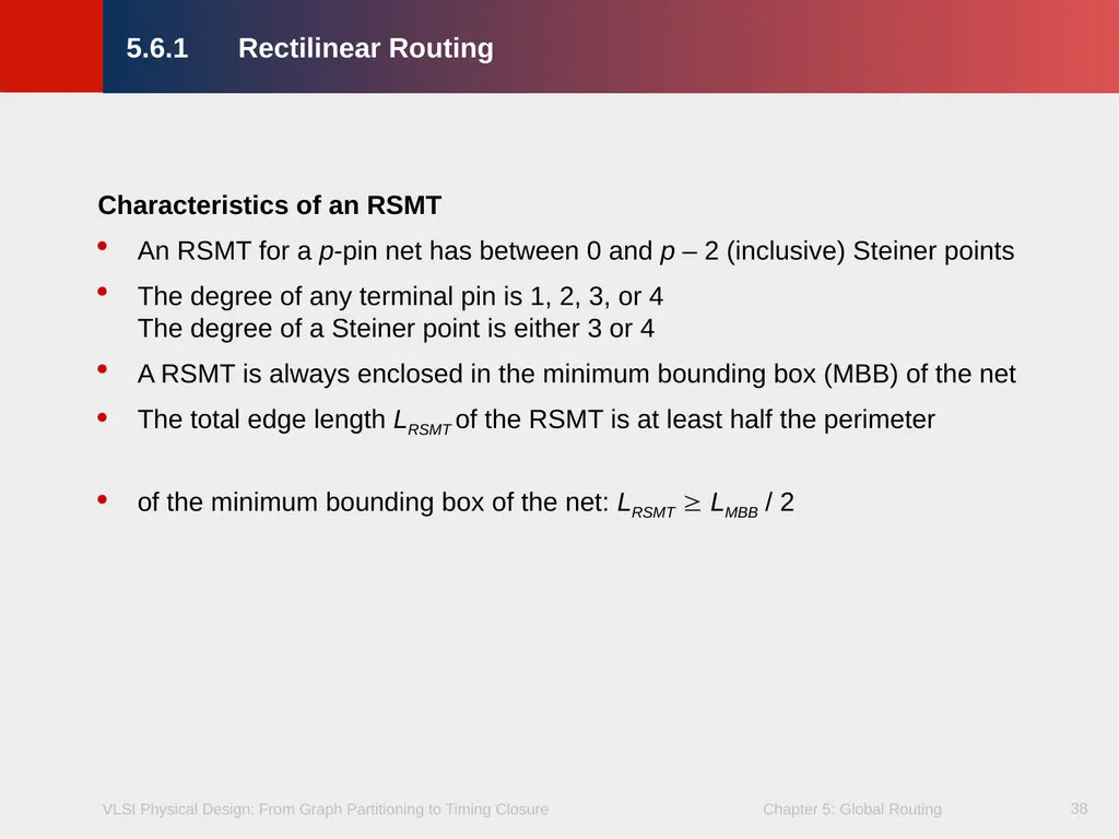
slide38. 38 Characteristics of an RSMT
An RSMT for a p-pin net has between 0 and p – 2 (inclusive) Steiner points
The degree of any terminal pin is 1, 2, 3, or 4 The degree of a Steiner point is either 3 or 4
A RSMT is always enclosed in the minimum bounding box (MBB) of the net
The total edge length LRSMT of the RSMT is at least half the perimeter
of the minimum bounding box of the net: LRSMT LMBB / 2 5.6.1 Rectilinear Routing<br>
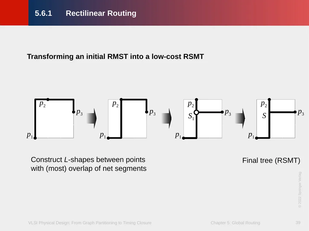
slide39. 39 Transforming an initial RMST into a low-cost RSMT 5.6.1 Rectilinear Routing © 2022 Springer Verlag<br>
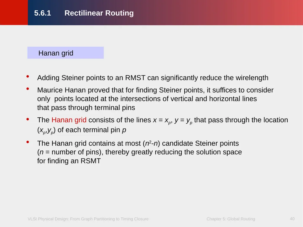
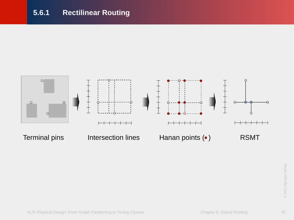
slide40. 40 Hanan grid
Adding Steiner points to an RMST can significantly reduce the wirelength
Maurice Hanan proved that for finding Steiner points, it suffices to consider only points located at the intersections of vertical and horizontal lines that pass through terminal pins
The Hanan grid consists of the lines x = xp, y = yp that pass through the location (xp,yp) of each terminal pin p
The Hanan grid contains at most (n2-n) candidate Steiner points (n = number of pins), thereby greatly reducing the solution space for finding an RSMT 5.6.1 Rectilinear Routing<br>
slide41. 41 5.6.1 Rectilinear Routing © 2022 Springer Verlag<br>
slide42. 42 5.6.1 Rectilinear Routing<br>
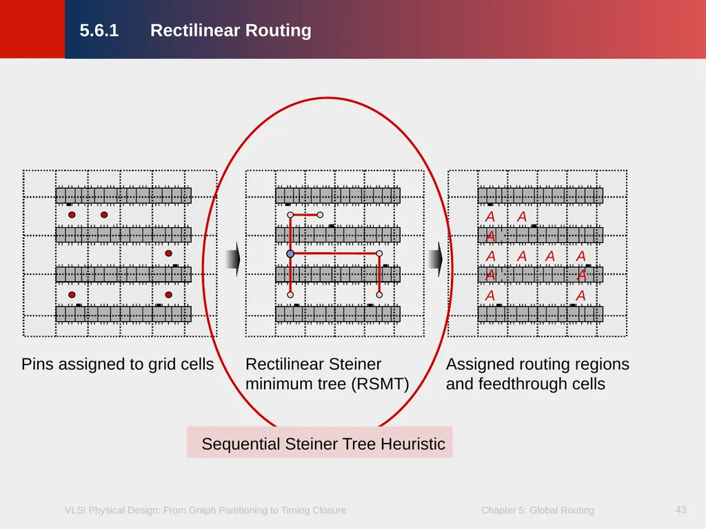
slide43. 43 Sequential Steiner Tree Heuristic 5.6.1 Rectilinear Routing<br>
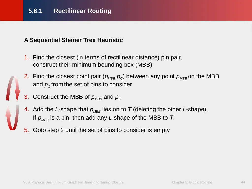
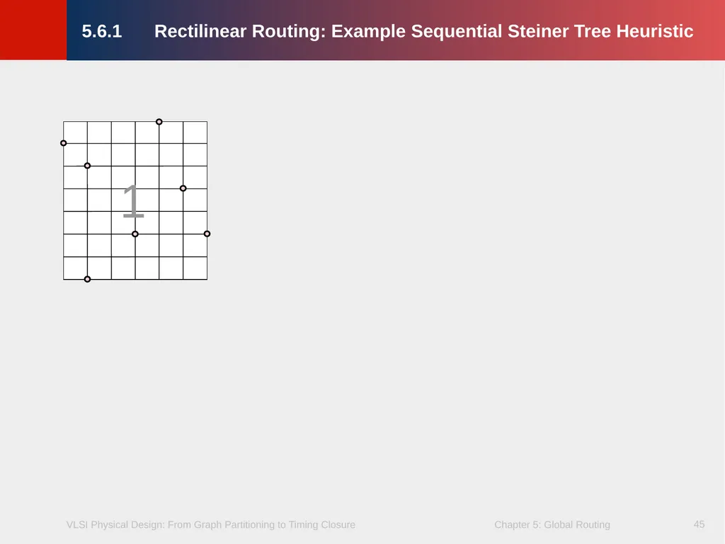
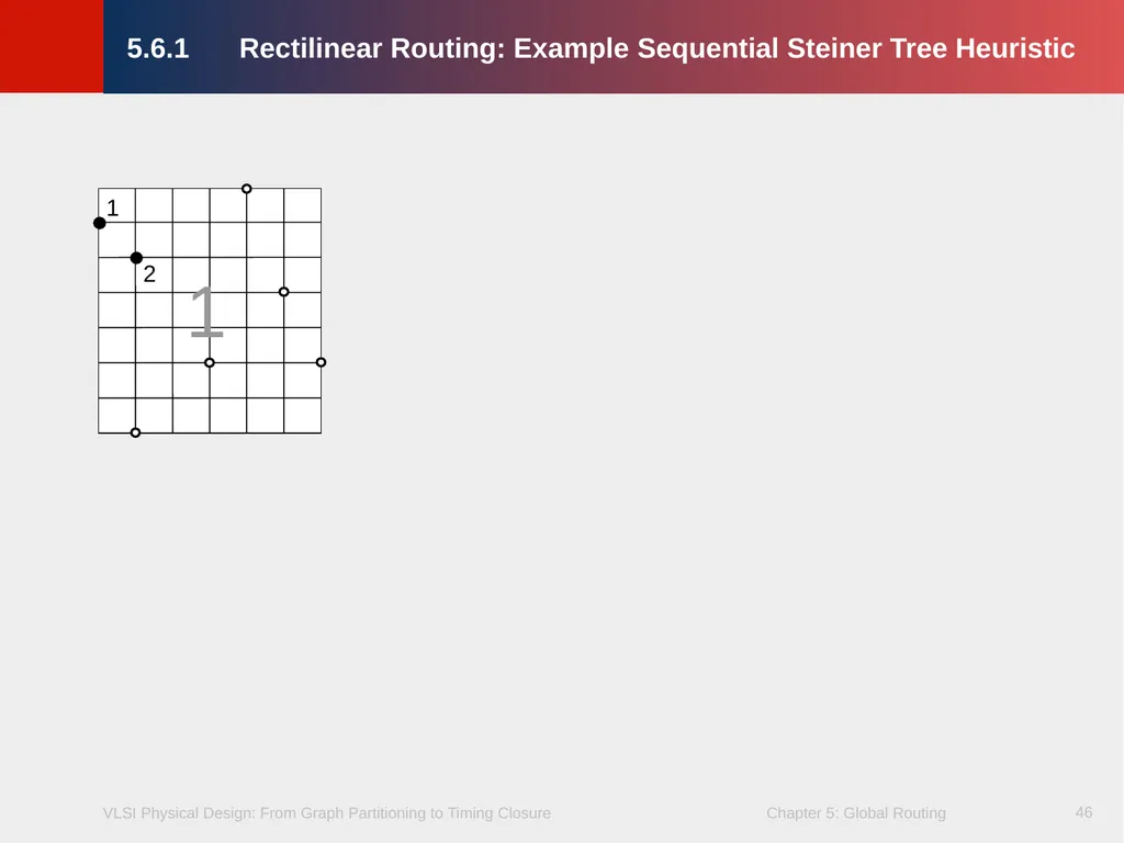
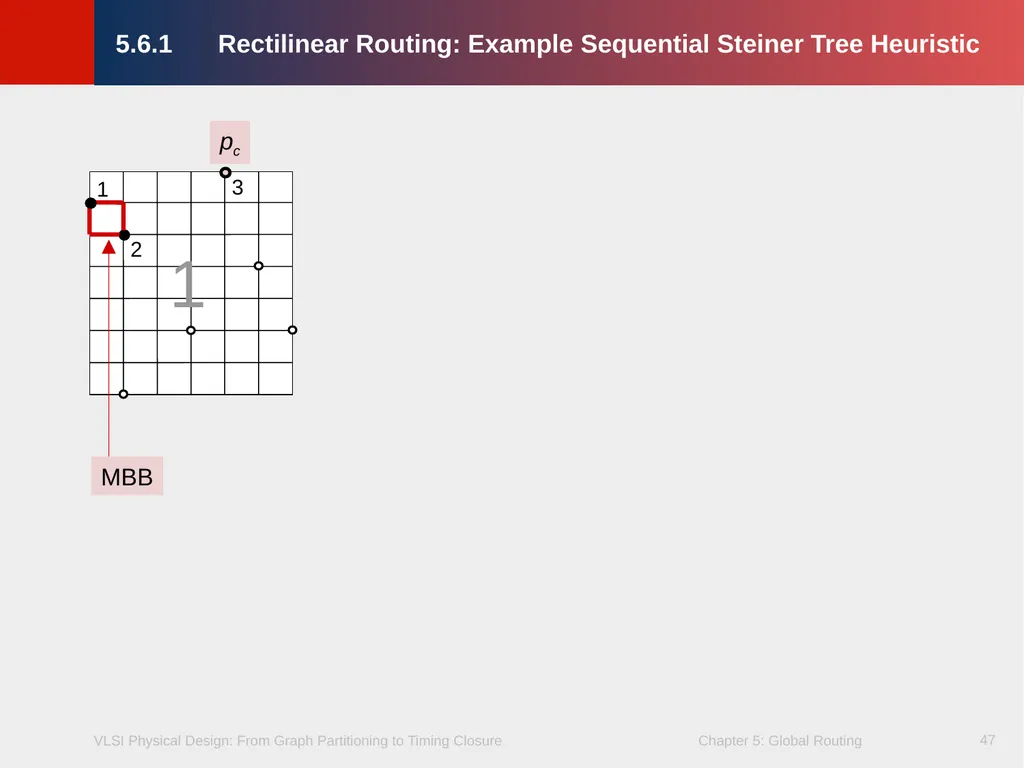
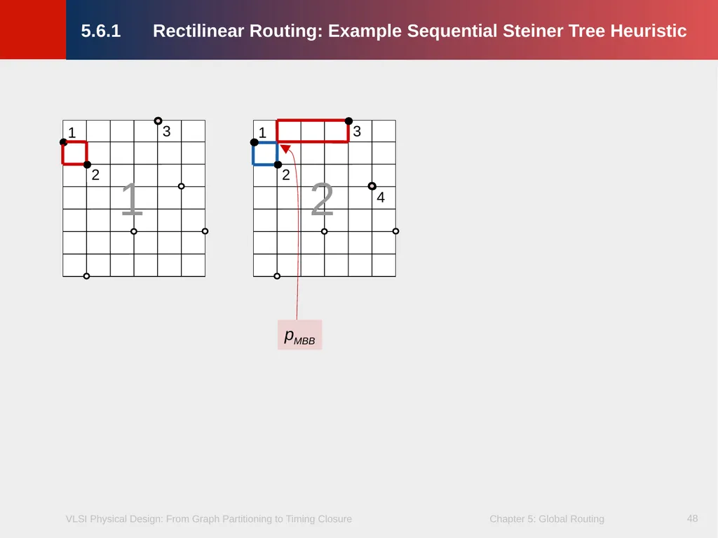
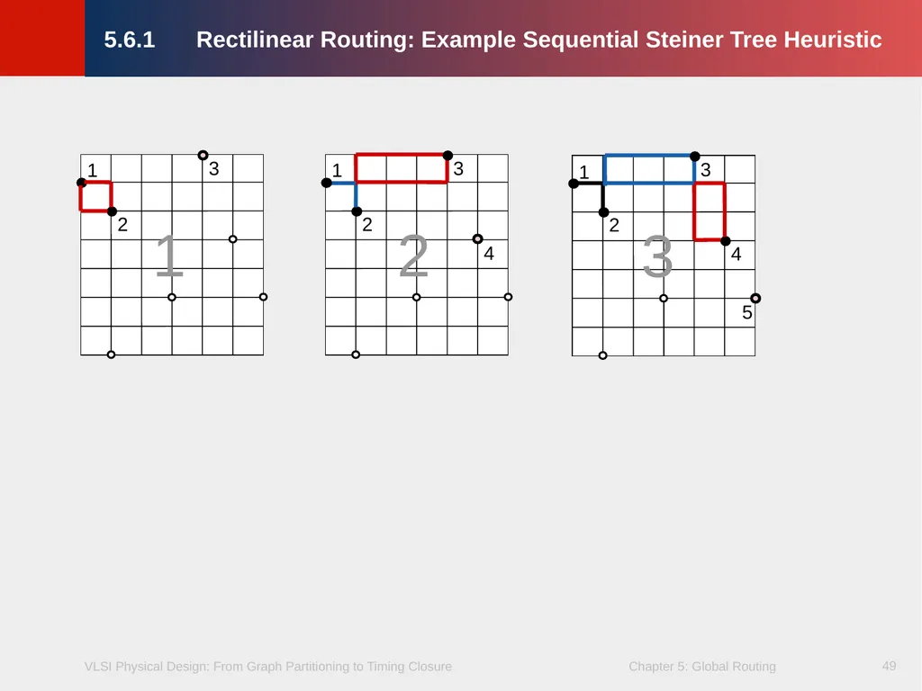
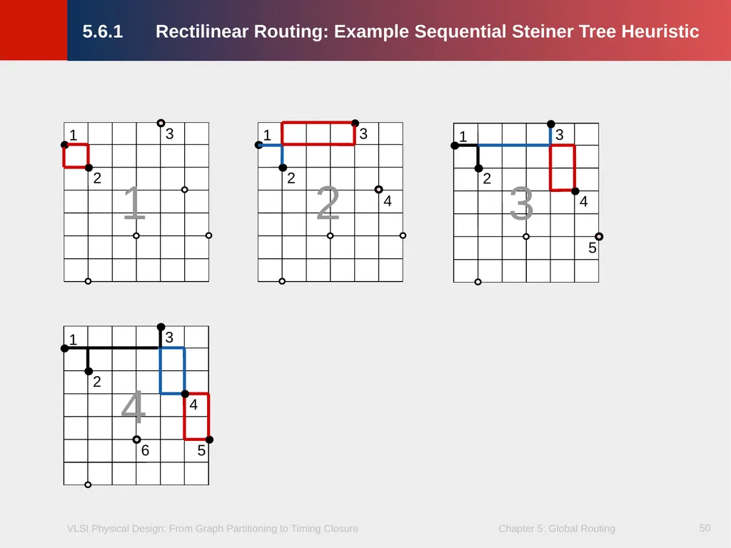
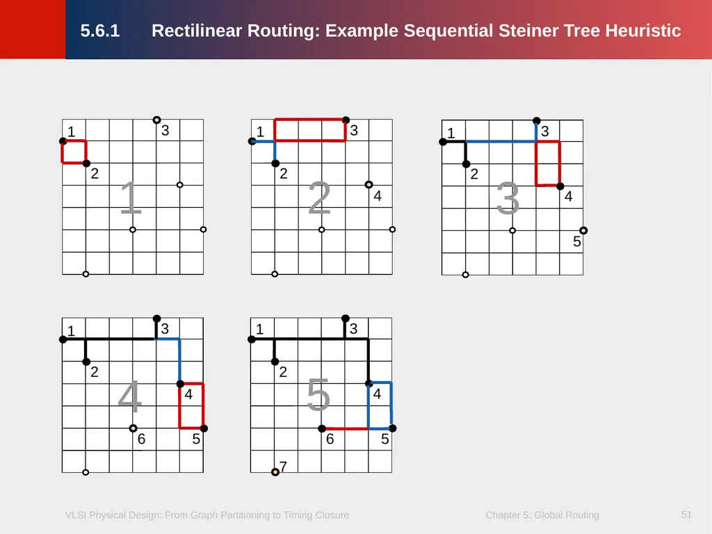
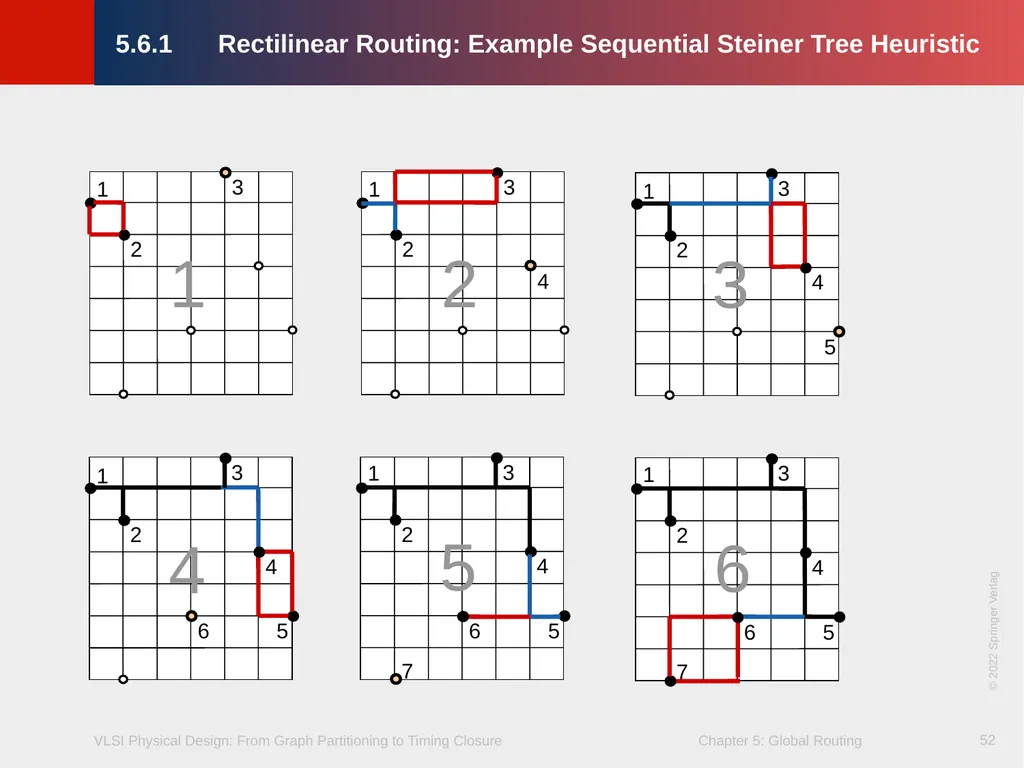
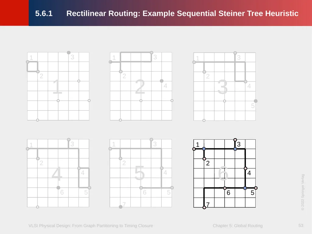
slide44. 44 A Sequential Steiner Tree Heuristic
Find the closest (in terms of rectilinear distance) pin pair, construct their minimum bounding box (MBB)
Find the closest point pair (pMBB,pC) between any point pMBB on the MBB and pC from the set of pins to consider
Construct the MBB of pMBB and pC
Add the L-shape that pMBB lies on to T (deleting the other L-shape). If pMBB is a pin, then add any L-shape of the MBB to T.
Goto step 2 until the set of pins to consider is empty 5.6.1 Rectilinear Routing<br>
slide45. 45 1 5.6.1 Rectilinear Routing: Example Sequential Steiner Tree Heuristic<br>
slide46. 46 1 2 1 5.6.1 Rectilinear Routing: Example Sequential Steiner Tree Heuristic<br>
slide47. 47 1 2 3 1 5.6.1 Rectilinear Routing: Example Sequential Steiner Tree Heuristic MBB pc<br>
slide48. 48 1 2 3 1 2 3 1 2 4 5.6.1 Rectilinear Routing: Example Sequential Steiner Tree Heuristic pMBB<br>
slide49. 49 1 2 3 1 2 3 4 5 1 2 3 4 1 2 3 5.6.1 Rectilinear Routing: Example Sequential Steiner Tree Heuristic<br>
slide50. 50 1 2 3 1 2 3 4 5 1 2 3 4 1 2 3 4 5 6 1 2 3 4 5.6.1 Rectilinear Routing: Example Sequential Steiner Tree Heuristic<br>
slide51. 51 1 2 3 4 5 6 7 1 2 3 1 2 3 4 5 1 2 3 4 1 2 3 4 5 6 1 2 3 4 5 5.6.1 Rectilinear Routing: Example Sequential Steiner Tree Heuristic<br>
slide52. 52 1 2 3 4 5 6 7 1 2 3 1 2 3 4 5 1 2 3 4 5 6 7 1 2 3 4 1 2 3 4 5 6 1 2 3 4 5 6 5.6.1 Rectilinear Routing: Example Sequential Steiner Tree Heuristic © 2022 Springer Verlag<br>
slide53. 53 1 2 3 4 5 6 7 1 2 3 1 2 3 4 5 1 2 3 4 5 6 7 1 2 3 4 1 2 3 4 5 6 1 2 3 4 5 6 5.6.1 Rectilinear Routing: Example Sequential Steiner Tree Heuristic © 2022 Springer Verlag<br>
slide54. 54 1 2 3 4 5 6 7 8 9 1 2 3 4 5 6 7 8 9 10 11 12 13 14 Channel connectivity graph Switchbox connectivity graph 5.6.2 Global Routing in a Connectivity Graph<br>
slide55. 55 5.6.2 Global Routing in a Connectivity Graph Channel connectivity graph Switchbox connectivity graph<br>
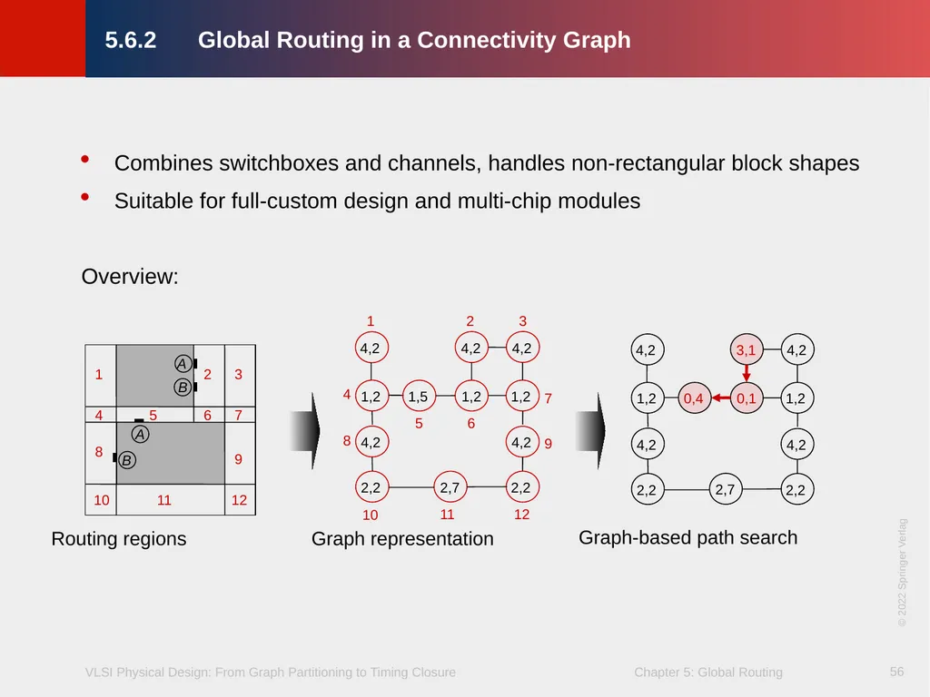
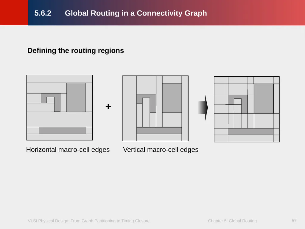
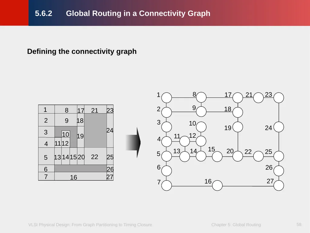
slide56. 56 Combines switchboxes and channels, handles non-rectangular block shapes
Suitable for full-custom design and multi-chip modules
Overview: 5.6.2 Global Routing in a Connectivity Graph © 2022 Springer Verlag<br>
slide57. 57 Horizontal macro-cell edges Vertical macro-cell edges Defining the routing regions 5.6.2 Global Routing in a Connectivity Graph +<br>
slide58. 58 2 3 4 5 6 7 8 9 10 11 12 13 14 15 16 17 18 19 20 21 22 23 24 25 26 27 1 2 3 4 5 6 7 8 9 10 11 12 13 14 15 16 17 18 19 20 21 22 23 24 25 26 27 1 Defining the connectivity graph 5.6.2 Global Routing in a Connectivity Graph<br>
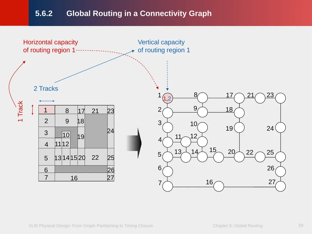
slide59. 59 2 3 4 5 6 7 8 9 10 11 12 13 14 15 16 17 18 19 20 21 22 23 24 25 26 27 1 2 3 4 5 6 7 8 9 10 11 12 13 14 15 16 17 18 19 20 21 22 23 24 25 26 27 1,2 Horizontal capacity of routing region 1 Vertical capacity of routing region 1 2 Tracks 1 Track 1 5.6.2 Global Routing in a Connectivity Graph<br>
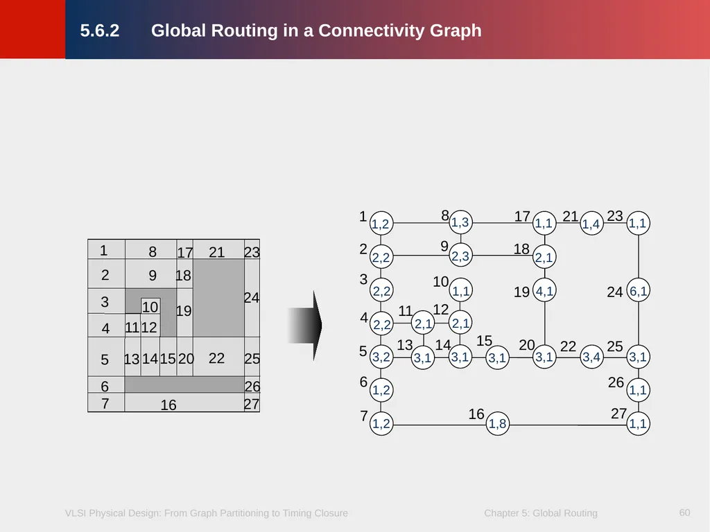
slide60. 60 2 3 4 5 6 7 8 9 10 11 12 13 14 15 16 17 18 19 20 21 22 23 24 25 26 27 1 2 3 4 5 6 7 8 9 10 11 12 13 14 15 16 17 18 19 20 21 22 23 24 25 26 27 1,2 2,2 2,2 2,2 3,2 1,2 1,2 2,1 3,1 1,3 2,3 1,1 2,1 3,1 3,1 1,1 2,1 4,1 3,1 1,1 6,1 3,1 1,1 1,1 1,4 3,4 1,8 1 5.6.2 Global Routing in a Connectivity Graph<br>
slide61. 61 Algorithm Overview
Define routing regions
Define connectivity graph
Determine net ordering
Assign tracks for all pin connections in Netlist
Consider each net
Free corresponding tracks for net’s pins
Decompose net into two-pin subnets
Find shortest path for subnet connectivity graph
If no shortest path exists, do not route, otherwise, assign subnet to the nodes of shortest path and update routing capacities
If there are unrouted nets, goto Step 5, otherwise END 5.6.2 Global Routing in a Connectivity Graph<br>
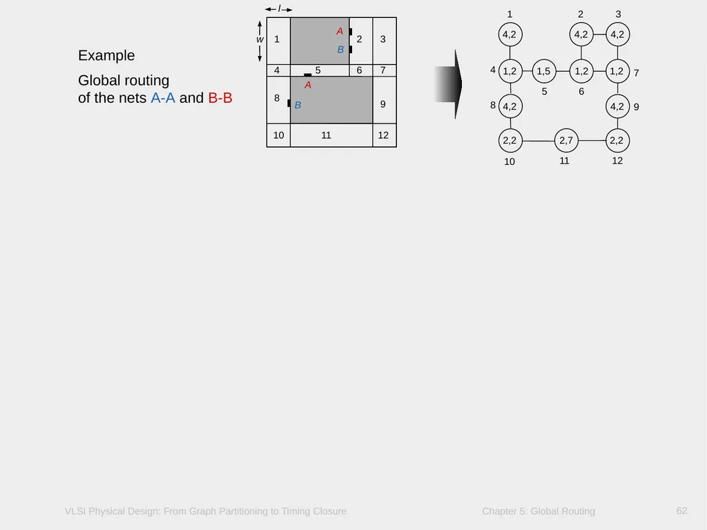
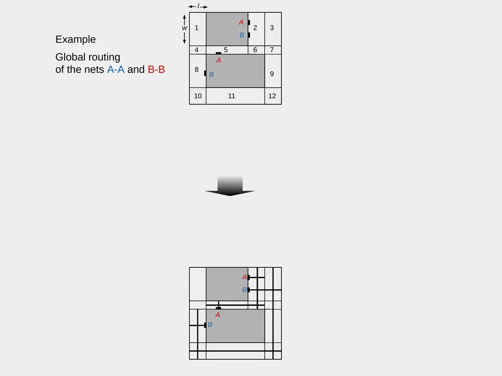
slide62. 62 l 1 2 3 4 5 6 7 8 9 10 11 12 B A B A w Example
Global routing of the nets A-A and B-B<br>
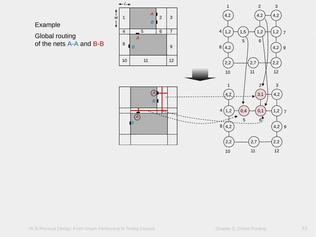
slide63. 63 l 1 2 3 4 5 6 7 8 9 10 11 12 B A B A w 1 2 3 4 2,2 4,2 1,2 2,7 4,2 1,2 1,2 5 6 8 4,2 7 2,2 4,2 9 10 4,2 1,5 11 12 B A B A 0,1 3,1 0,4 Example
Global routing of the nets A-A and B-B<br>
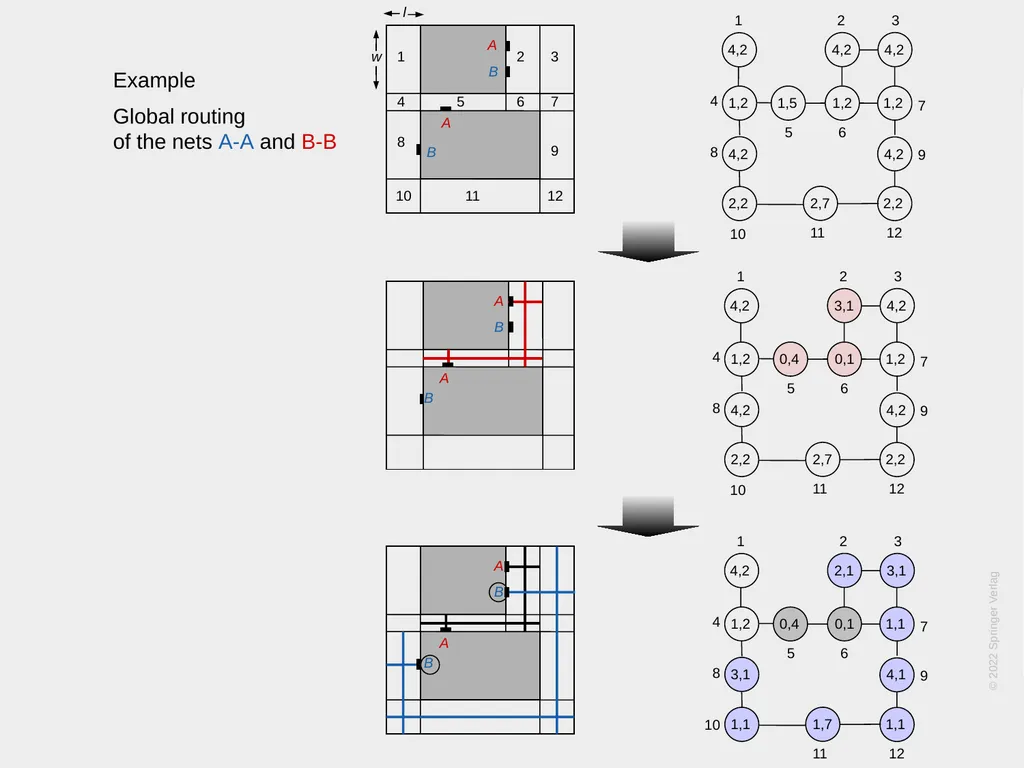
slide64. 64 l 1 2 3 4 5 6 7 8 9 10 11 12 B A B A w 1 2 3 4 2,2 4,2 1,2 2,7 4,2 1,2 1,2 5 6 8 4,2 7 2,2 4,2 9 10 4,2 1,5 11 12 B A B A B A B A 1 2 3 4 2,2 4,2 1,2 2,7 4,2 0,1 1,2 5 6 8 3,1 7 2,2 4,2 9 10 4,2 0,4 11 12 Example
Global routing of the nets A-A and B-B © 2022 Springer Verlag<br>
slide65. 65 l 1 2 3 4 5 6 7 8 9 10 11 12 B A B A w B A B A Example
Global routing of the nets A-A and B-B<br>
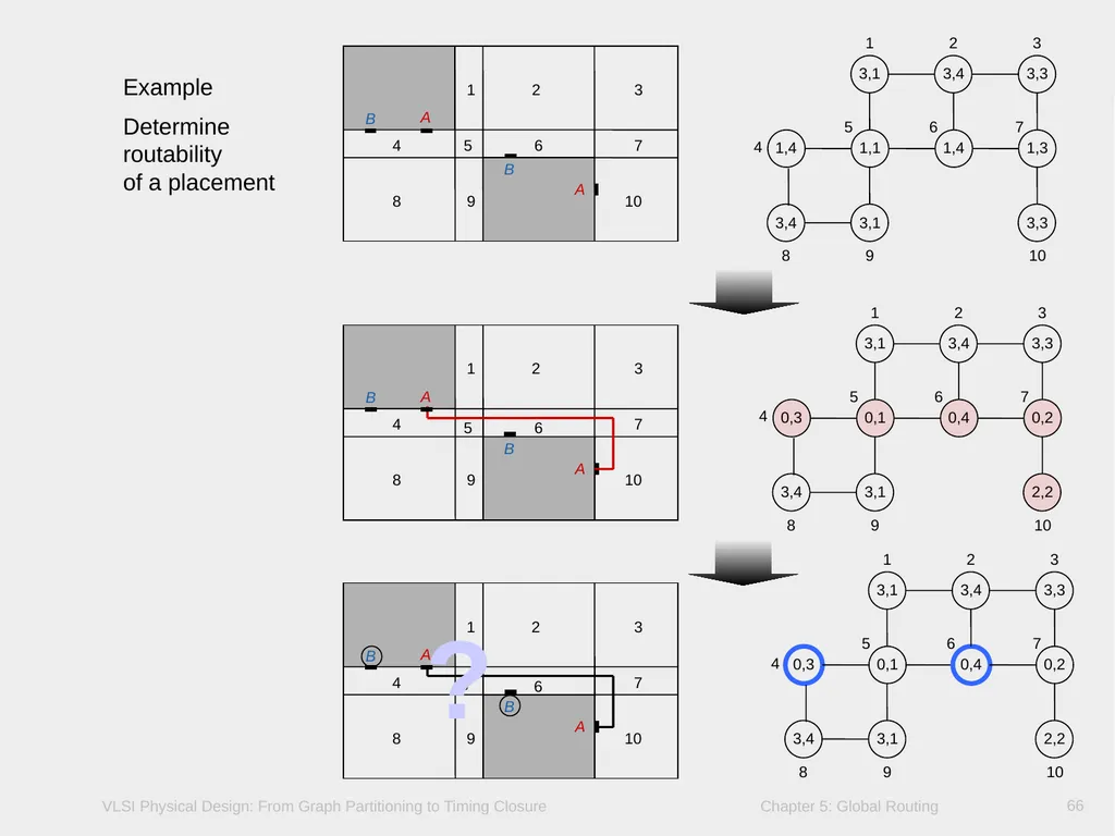
slide66. 66 B A B A 4 5 7 8 6 9 10 1 2 3 Example
Determine routability of a placement ?<br>
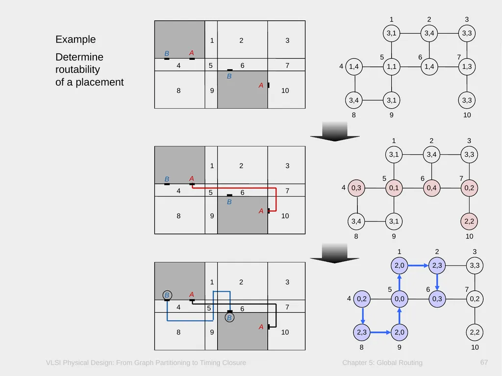
slide67. 67 B A B A 4 5 7 8 6 9 10 1 2 3 B A B A 4 5 7 8 6 9 10 1 2 3 B A B A 4 5 7 8 6 9 10 1 2 3 1 2 3 3,1 3,4 3,3 0,3 0,1 0,4 0,2 3,4 3,1 2,2 4 5 6 7 8 9 10 1 2 3 2,0 2,3 3,3 0,2 0,0 0,3 0,2 2,3 2,0 2,2 4 5 6 7 8 9 10 Example
Determine routability of a placement<br>
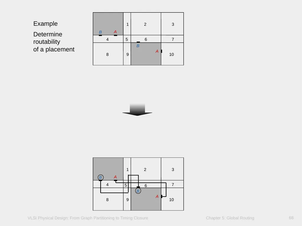
slide68. 68 B A B A 4 5 7 8 6 9 10 1 2 3 B A B A 4 5 7 8 6 9 10 1 2 3 Example
Determine routability of a placement<br>
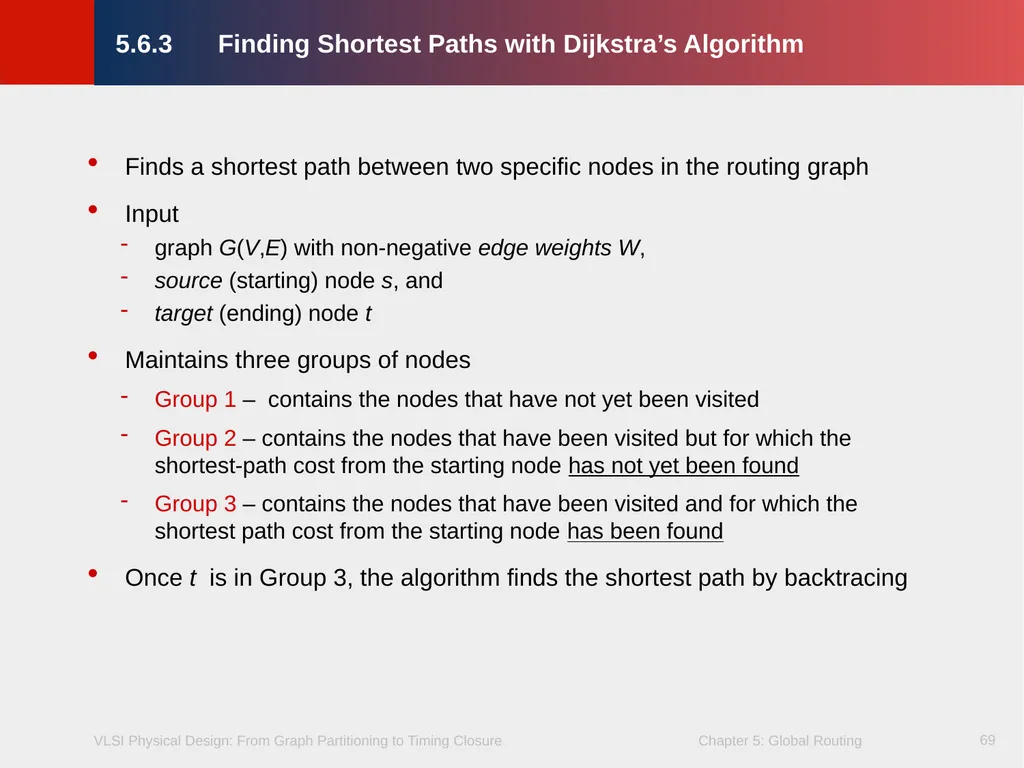
slide69. 69 Finds a shortest path between two specific nodes in the routing graph
Input
graph G(V,E) with non-negative edge weights W,
source (starting) node s, and
target (ending) node t
Maintains three groups of nodes
Group 1 – contains the nodes that have not yet been visited
Group 2 – contains the nodes that have been visited but for which the shortest-path cost from the starting node has not yet been found
Group 3 – contains the nodes that have been visited and for which the shortest path cost from the starting node has been found
Once t is in Group 3, the algorithm finds the shortest path by backtracing 5.6.3 Finding Shortest Paths with Dijkstra’s Algorithm<br>
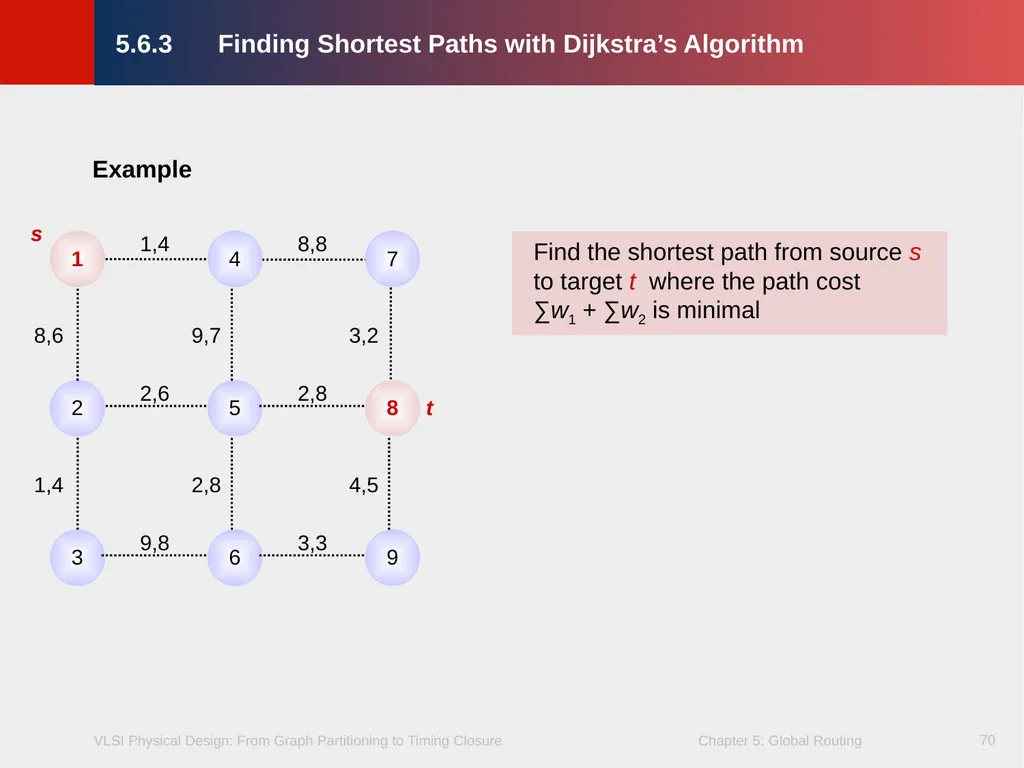
slide70. 70 1 4 7 2 5 8 3 6 9 s t 1,4 8,8 2,6 2,8 9,8 3,3 8,6 9,7 3,2 1,4 2,8 4,5 Find the shortest path from source s to target t where the path cost ∑w1 + ∑w2 is minimal 5.6.3 Finding Shortest Paths with Dijkstra’s Algorithm Example<br>
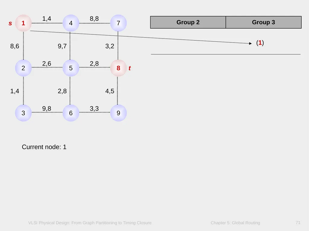
slide71. 71 1 4 7 2 5 8 3 6 9 s t 1,4 8,8 2,6 2,8 9,8 3,3 8,6 9,7 3,2 1,4 2,8 4,5 (1) Current node: 1<br>
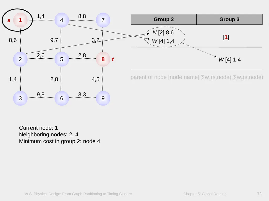
slide72. 72 [1] N [2] 8,6 W [4] 1,4 W [4] 1,4 parent of node [node name] ∑w1(s,node),∑w2(s,node) 1 4 7 2 5 8 3 6 9 1,4 8,8 2,6 2,8 9,8 3,3 8,6 9,7 3,2 1,4 2,8 4,5 Current node: 1 Neighboring nodes: 2, 4 Minimum cost in group 2: node 4 s t<br>
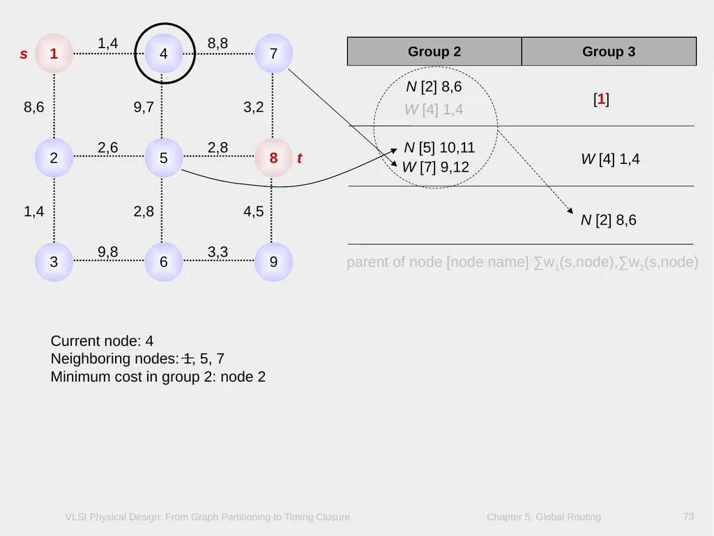
slide73. 73 1 4 7 2 5 8 3 6 9 1,4 8,8 2,6 2,8 9,8 3,3 8,6 9,7 3,2 1,4 2,8 4,5 [1] N [2] 8,6 W [4] 1,4 W [4] 1,4 N [5] 10,11 W [7] 9,12 N [2] 8,6 Current node: 4
Neighboring nodes: 1, 5, 7 Minimum cost in group 2: node 2 s t parent of node [node name] ∑w1(s,node),∑w2(s,node)<br>
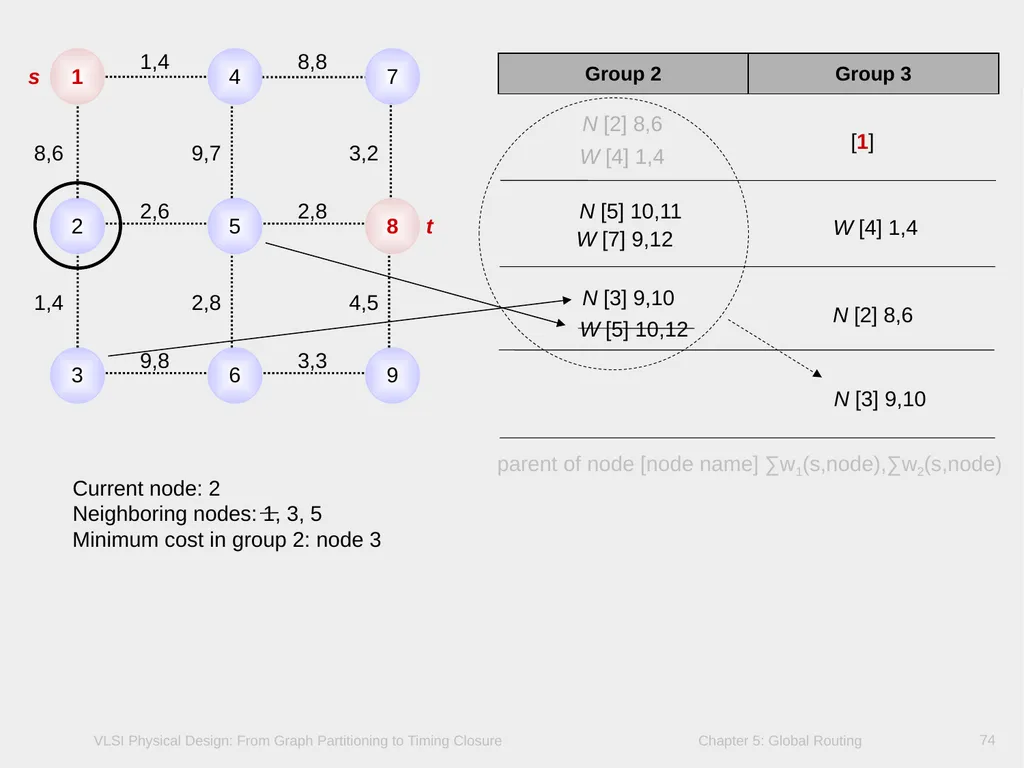
slide74. 74 1 4 7 2 5 8 3 6 9 1,4 8,8 2,6 2,8 9,8 3,3 8,6 9,7 3,2 1,4 2,8 4,5 [1] N [2] 8,6 W [4] 1,4 W [4] 1,4 N [5] 10,11 W [7] 9,12 N [2] 8,6 N [3] 9,10 W [5] 10,12 N [3] 9,10 Current node: 2
Neighboring nodes: 1, 3, 5 Minimum cost in group 2: node 3 s t parent of node [node name] ∑w1(s,node),∑w2(s,node)<br>
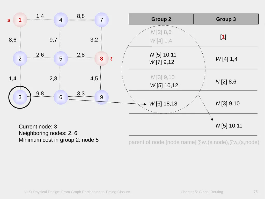
slide75. 75 1 4 7 2 5 8 3 6 9 1,4 8,8 2,6 2,8 9,8 3,3 8,6 9,7 3,2 1,4 2,8 4,5 [1] N [2] 8,6 W [4] 1,4 W [4] 1,4 N [5] 10,11 W [7] 9,12 N [2] 8,6 N [3] 9,10 W [5] 10,12 N [3] 9,10 W [6] 18,18 N [5] 10,11 Current node: 3
Neighboring nodes: 2, 6 Minimum cost in group 2: node 5 s t parent of node [node name] ∑w1(s,node),∑w2(s,node)<br>
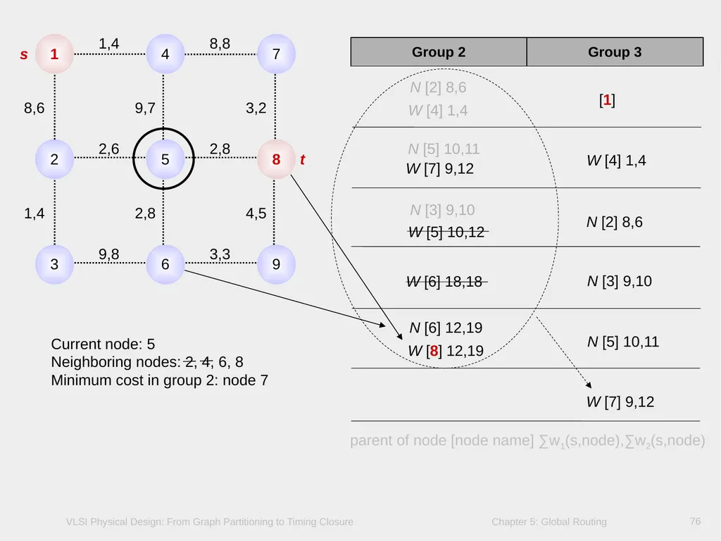
slide76. 76 1 4 7 2 5 8 3 6 9 1,4 8,8 2,6 2,8 9,8 3,3 8,6 9,7 3,2 1,4 2,8 4,5 [1] N [2] 8,6 W [4] 1,4 W [4] 1,4 N [5] 10,11 W [7] 9,12 N [2] 8,6 N [3] 9,10 W [5] 10,12 N [3] 9,10 W [6] 18,18 N [5] 10,11 N [6] 12,19 W [8] 12,19 W [7] 9,12 Current node: 5
Neighboring nodes: 2, 4, 6, 8 Minimum cost in group 2: node 7 s t parent of node [node name] ∑w1(s,node),∑w2(s,node)<br>
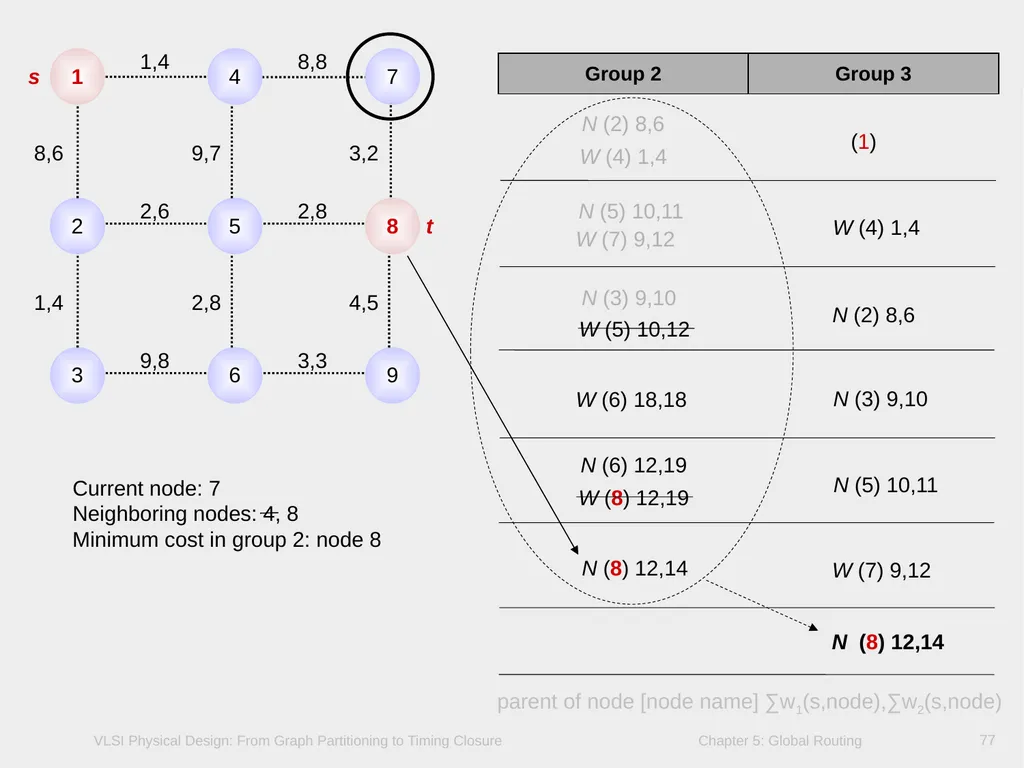
slide77. 77 1 4 7 2 5 8 3 6 9 1,4 8,8 2,6 2,8 9,8 3,3 8,6 9,7 3,2 1,4 2,8 4,5 (1) N (2) 8,6 W (4) 1,4 W (4) 1,4 N (5) 10,11 W (7) 9,12 N (2) 8,6 N (3) 9,10 W (5) 10,12 N (3) 9,10 W (6) 18,18 N (5) 10,11 N (6) 12,19 W (8) 12,19 W (7) 9,12 N (8) 12,14 N (8) 12,14 Current node: 7
Neighboring nodes: 4, 8 Minimum cost in group 2: node 8 s t parent of node [node name] ∑w1(s,node),∑w2(s,node)<br>
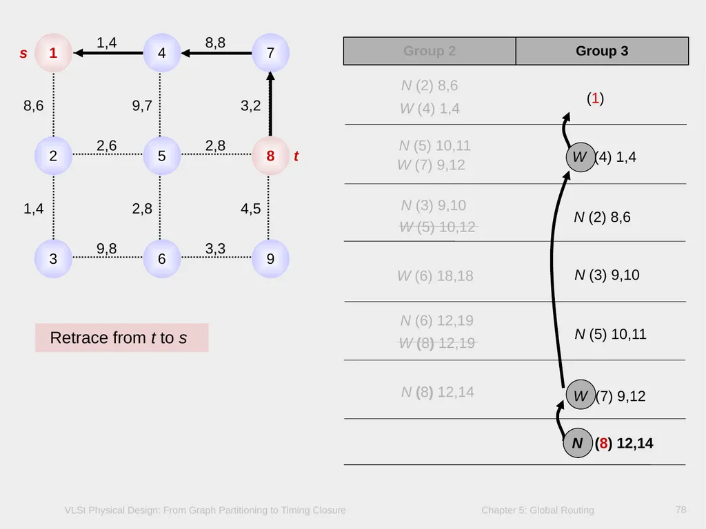
slide78. 78 1 7 2 5 8 3 6 9 1,4 8,8 2,6 2,8 9,8 3,3 8,6 9,7 3,2 1,4 2,8 4,5 (1) N (2) 8,6 W (4) 1,4 W (4) 1,4 N (5) 10,11 W (7) 9,12 N (2) 8,6 N (3) 9,10 W (5) 10,12 N (3) 9,10 W (6) 18,18 N (5) 10,11 N (6) 12,19 W (8) 12,19 W (7) 9,12 N (8) 12,14 N (8) 12,14 Retrace from t to s s t 4<br>
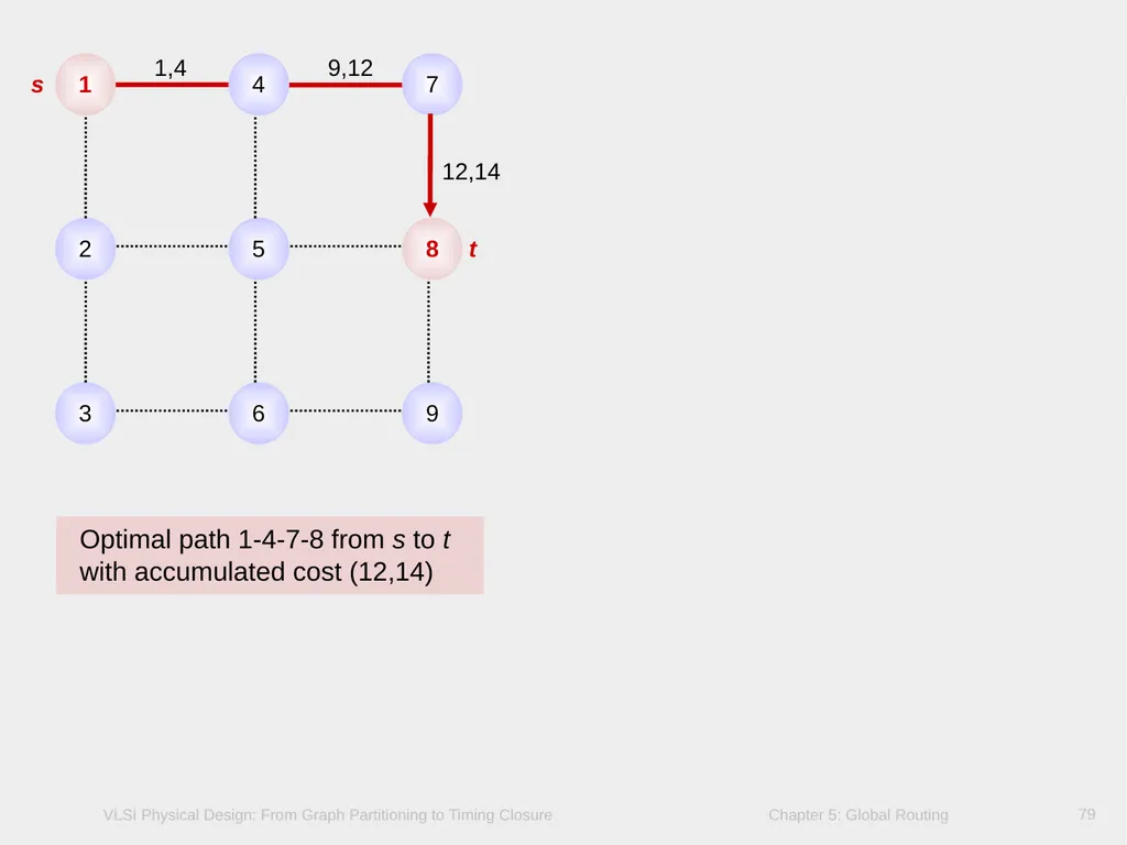
slide79. 79 1 4 7 2 5 8 3 6 9 1,4 9,12 12,14 Optimal path 1-4-7-8 from s to t with accumulated cost (12,14) s t<br>
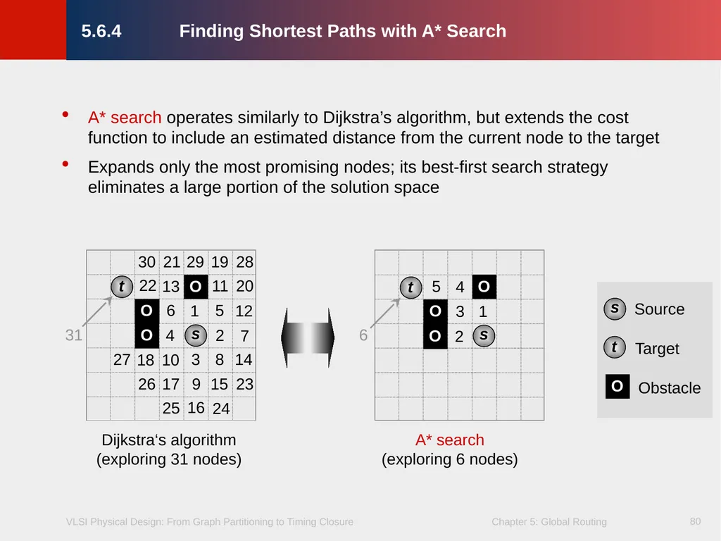
slide80. 80 5.6.4 Finding Shortest Paths with A* Search A* search operates similarly to Dijkstra’s algorithm, but extends the cost function to include an estimated distance from the current node to the target
Expands only the most promising nodes; its best-first search strategy eliminates a large portion of the solution space<br>
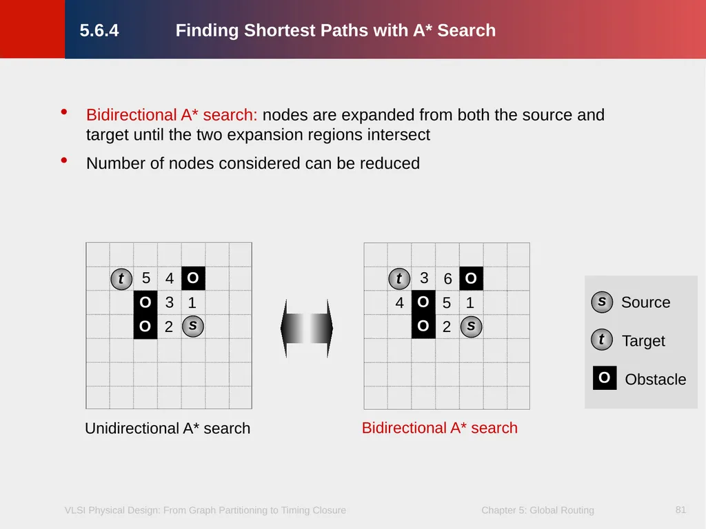
slide81. 81 5.6.4 Finding Shortest Paths with A* Search Bidirectional A* search: nodes are expanded from both the source and target until the two expansion regions intersect
Number of nodes considered can be reduced<br>
slide82. 82 5.1 Introduction
5.2 Terminology and Definitions
5.3 Optimization Goals
5.4 Representations of Routing Regions
5.5 The Global Routing Flow
5.6 Single-Net Routing
5.6.1 Rectilinear Routing
5.6.2 Global Routing in a Connectivity Graph
5.6.3 Finding Shortest Paths with Dijkstra’s Algorithm
5.6.4 Finding Shortest Paths with A* Search
5.7 Full-Netlist Routing
5.7.1 Routing by Integer Linear Programming
5.7.2 Rip-Up and Reroute (RRR)
5.8 Modern Global Routing
5.8.1 Pattern Routing
5.8.2 Negotiated-Congestion Routing 5.7 Full-Netlist Routing<br>
slide83. 83 5.7 Full-Netlist Routing Global routers must properly match nets with routing resources, without oversubscribing resources in any part of the chip
Signal nets are either routed
simultaneously, e.g., by integer linear programming, or
sequentially, e.g., one net at a time
When certain nets cause resource contention or overflow for routing edges, sequential routing requires multiple iterations: rip-up and reroute<br>
slide84. 84 5.7.1 Routing by Integer Linear Programming A linear program (LP) consists
of a set of constraints and
an optional objective function
Objective function is maximized or minimized
Both the constraints and the objective function must be linear
Constraints form a system of linear equations and inequalities
Integer linear program (ILP): linear program where every variable can only assume integer values
Typically takes much longer to solve
In many cases, variables are only allowed values 0 and 1
Several ways to formulate the global routing problem as an ILP, one of which is presented next<br>
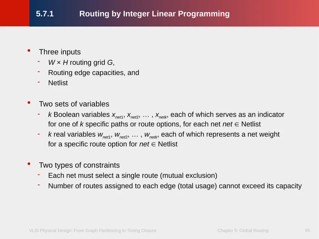
slide85. 85 5.7.1 Routing by Integer Linear Programming Three inputs
W × H routing grid G,
Routing edge capacities, and
Netlist
Two sets of variables
k Boolean variables xnet1, xnet2, … , xnetk, each of which serves as an indicator for one of k specific paths or route options, for each net net Netlist
k real variables wnet1, wnet2, … , wnetk, each of which represents a net weight for a specific route option for net Netlist
Two types of constraints
Each net must select a single route (mutual exclusion)
Number of routes assigned to each edge (total usage) cannot exceed its capacity<br>
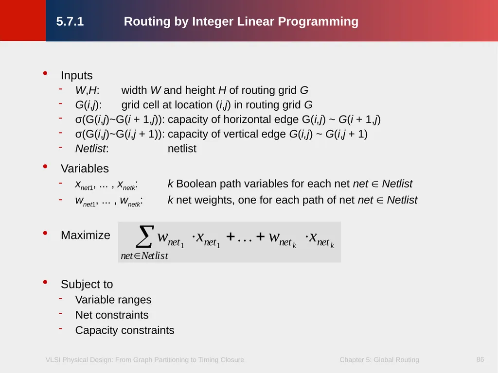
slide86. 86 5.7.1 Routing by Integer Linear Programming Inputs
W,H: width W and height H of routing grid G
G(i,j): grid cell at location (i,j) in routing grid G
σ(G(i,j)~G(i + 1,j)): capacity of horizontal edge G(i,j) ~ G(i + 1,j)
σ(G(i,j)~G(i,j + 1)): capacity of vertical edge G(i,j) ~ G(i,j + 1)
Netlist: netlist
Variables
xnet1, ... , xnetk: k Boolean path variables for each net net Netlist
wnet1, ... , wnetk: k net weights, one for each path of net net Netlist
Maximize
Subject to
Variable ranges
Net constraints
Capacity constraints<br>
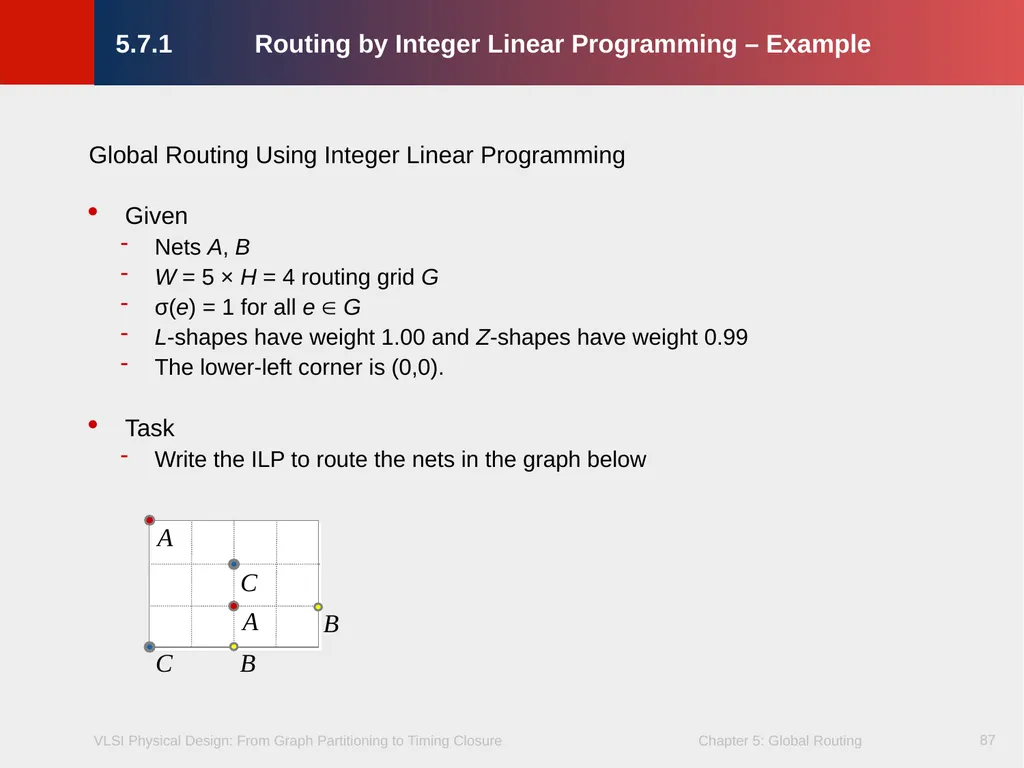
slide87. 87 5.7.1 Routing by Integer Linear Programming – Example Global Routing Using Integer Linear Programming
Given
Nets A, B
W = 5 × H = 4 routing grid G
σ(e) = 1 for all e G
L-shapes have weight 1.00 and Z-shapes have weight 0.99
The lower-left corner is (0,0).
Task
Write the ILP to route the nets in the graph below<br>
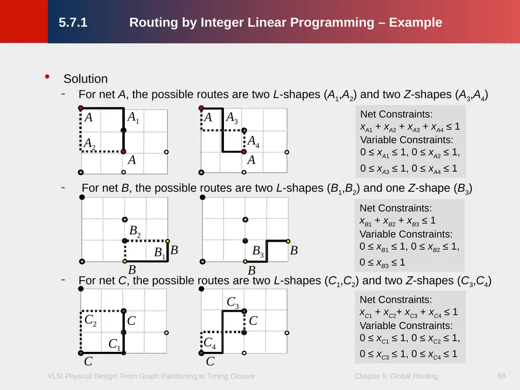
slide88. 88 5.7.1 Routing by Integer Linear Programming – Example Solution
For net A, the possible routes are two L-shapes (A1,A2) and two Z-shapes (A3,A4)
For net B, the possible routes are two L-shapes (B1,B2) and one Z-shape (B3)
For net C, the possible routes are two L-shapes (C1,C2) and two Z-shapes (C3,C4)<br>
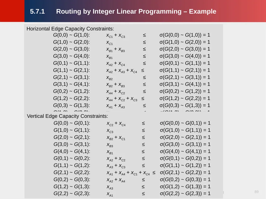
slide89. 89 5.7.1 Routing by Integer Linear Programming – Example Horizontal Edge Capacity Constraints:
G(0,0) ~ G(1,0): xC1 + xC3 ≤ σ(G(0,0) ~ G(1,0)) = 1
G(1,0) ~ G(2,0): xC1 ≤ σ(G(1,0) ~ G(2,0)) = 1
G(2,0) ~ G(3,0): xB1 + xB3 ≤ σ(G(2,0) ~ G(3,0)) = 1
G(3,0) ~ G(4,0): xB1 ≤ σ(G(3,0) ~ G(4,0)) = 1
G(0,1) ~ G(1,1): xA2 + xC4 ≤ σ(G(0,1) ~ G(1,1)) = 1
G(1,1) ~ G(2,1): xA2 + xA3 + xC4 ≤ σ(G(1,1) ~ G(2,1)) = 1
G(2,1) ~ G(3,1): xB2 ≤ σ(G(2,1) ~ G(3,1)) = 1
G(3,1) ~ G(4,1): xB2 + xB3 ≤ σ(G(3,1) ~ G(4,1)) = 1
G(0,2) ~ G(1,2): xA4 + xC2 ≤ σ(G(0,2) ~ G(1,2)) = 1
G(1,2) ~ G(2,2): xA4 + xC2 + xC3 ≤ σ(G(1,2) ~ G(2,2)) = 1
G(0,3) ~ G(1,3): xA1 + xA3 ≤ σ(G(0,3) ~ G(1,3)) = 1
G(1,3) ~ G(2,3): xA1 ≤ σ(G(1,3) ~ G(2,3)) = 1 Vertical Edge Capacity Constraints:
G(0,0) ~ G(0,1): xC2 + xC4 ≤ σ(G(0,0) ~ G(0,1)) = 1
G(1,0) ~ G(1,1): xC3 ≤ σ(G(1,0) ~ G(1,1)) = 1
G(2,0) ~ G(2,1): xB2 + xC1 ≤ σ(G(2,0) ~ G(2,1)) = 1
G(3,0) ~ G(3,1): xB3 ≤ σ(G(3,0) ~ G(3,1)) = 1
G(4,0) ~ G(4,1): xB1 ≤ σ(G(4,0) ~ G(4,1)) = 1
G(0,1) ~ G(0,2): xA2 + xC2 ≤ σ(G(0,1) ~ G(0,2)) = 1
G(1,1) ~ G(1,2): xA3 + xC3 ≤ σ(G(1,1) ~ G(1,2)) = 1
G(2,1) ~ G(2,2): xA1 + xA4 + xC1 + xC4 ≤ σ(G(2,1) ~ G(2,2)) = 1
G(0,2) ~ G(0,3): xA2 + xA4 ≤ σ(G(0,2) ~ G(0,3)) = 1
G(1,2) ~ G(1,3): xA3 ≤ σ(G(1,2) ~ G(1,3)) = 1
G(2,2) ~ G(2,3): xA1 ≤ σ(G(2,2) ~ G(2,3)) = 1<br>
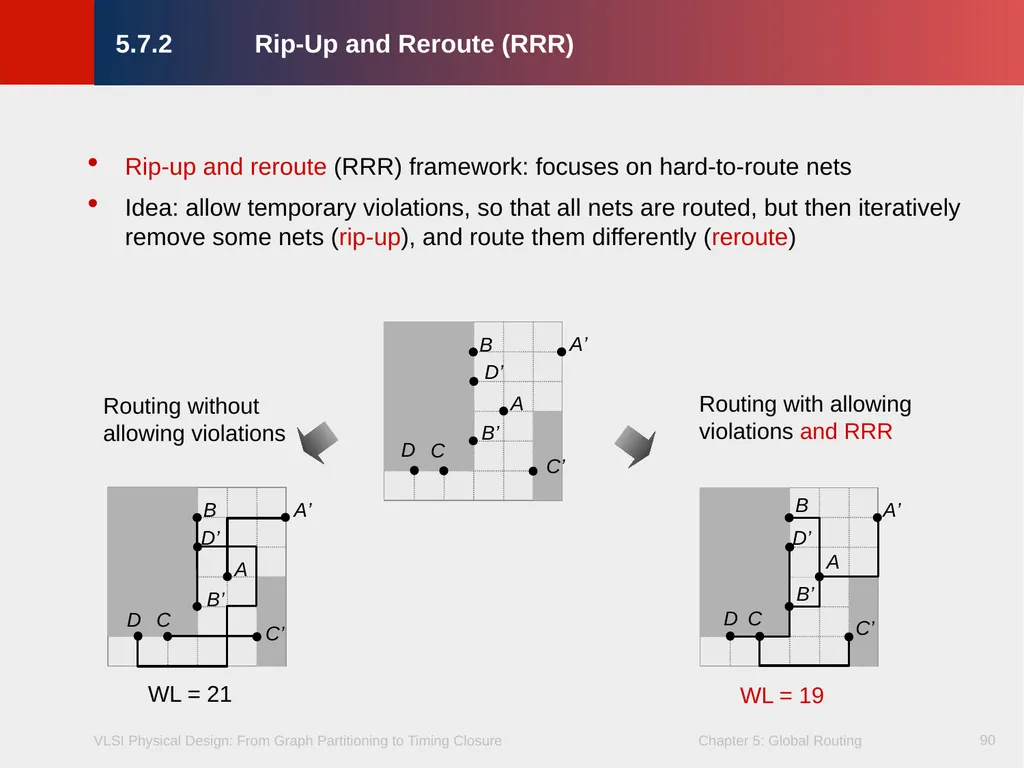
slide90. 90 5.7.2 Rip-Up and Reroute (RRR) Rip-up and reroute (RRR) framework: focuses on hard-to-route nets
Idea: allow temporary violations, so that all nets are routed, but then iteratively remove some nets (rip-up), and route them differently (reroute)<br>
slide91. 91 5.1 Introduction
5.2 Terminology and Definitions
5.3 Optimization Goals
5.4 Representations of Routing Regions
5.5 The Global Routing Flow
5.6 Single-Net Routing
5.6.1 Rectilinear Routing
5.6.2 Global Routing in a Connectivity Graph
5.6.3 Finding Shortest Paths with Dijkstra’s Algorithm
5.6.4 Finding Shortest Paths with A* Search
5.7 Full-Netlist Routing
5.7.1 Routing by Integer Linear Programming
5.7.2 Rip-Up and Reroute (RRR)
5.8 Modern Global Routing
5.8.1 Pattern Routing
5.8.2 Negotiated-Congestion Routing 5.8 Modern Global Routing<br>
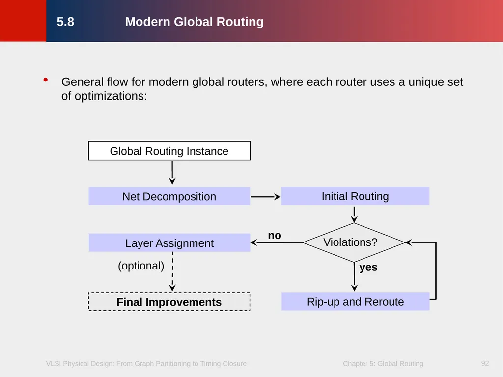
slide92. 92 General flow for modern global routers, where each router uses a unique set of optimizations: 5.8 Modern Global Routing<br>
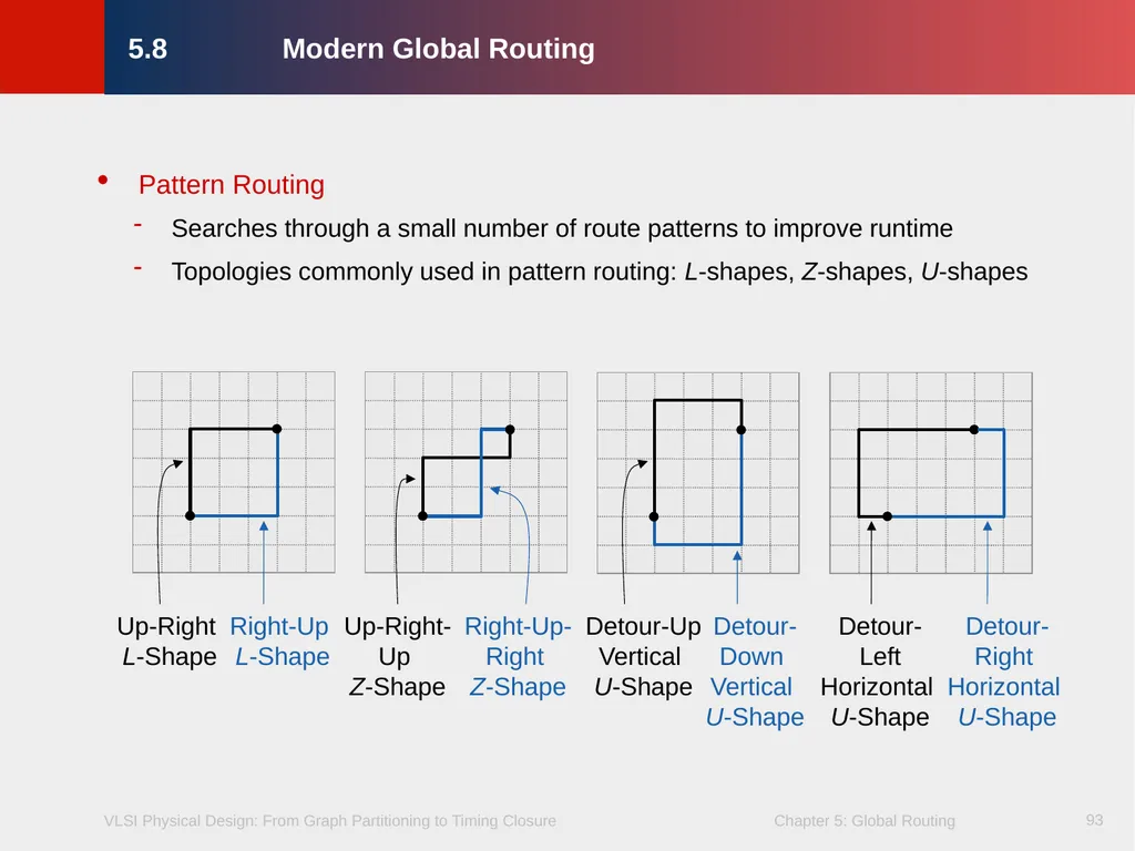
slide93. 93 Pattern Routing
Searches through a small number of route patterns to improve runtime
Topologies commonly used in pattern routing: L-shapes, Z-shapes, U-shapes 5.8 Modern Global Routing<br>
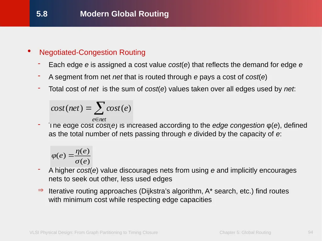
slide94. 94 Negotiated-Congestion Routing
Each edge e is assigned a cost value cost(e) that reflects the demand for edge e
A segment from net net that is routed through e pays a cost of cost(e)
Total cost of net is the sum of cost(e) values taken over all edges used by net:
The edge cost cost(e) is increased according to the edge congestion φ(e), defined as the total number of nets passing through e divided by the capacity of e:
A higher cost(e) value discourages nets from using e and implicitly encourages nets to seek out other, less used edges
Iterative routing approaches (Dijkstra’s algorithm, A* search, etc.) find routes with minimum cost while respecting edge capacities 5.8 Modern Global Routing<br>
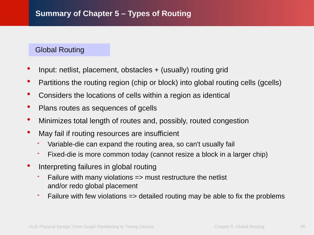
slide95. 95 Summary of Chapter 5 – Types of Routing Input: netlist, placement, obstacles + (usually) routing grid
Partitions the routing region (chip or block) into global routing cells (gcells)
Considers the locations of cells within a region as identical
Plans routes as sequences of gcells
Minimizes total length of routes and, possibly, routed congestion
May fail if routing resources are insufficient
Variable-die can expand the routing area, so can't usually fail
Fixed-die is more common today (cannot resize a block in a larger chip)
Interpreting failures in global routing
Failure with many violations => must restructure the netlist and/or redo global placement
Failure with few violations => detailed routing may be able to fix the problems Global Routing<br>
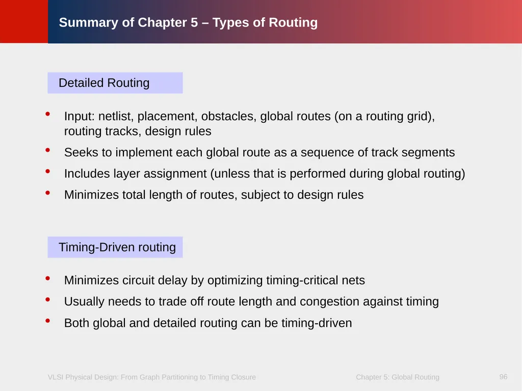
slide96. 96 Summary of Chapter 5 – Types of Routing Input: netlist, placement, obstacles, global routes (on a routing grid), routing tracks, design rules
Seeks to implement each global route as a sequence of track segments
Includes layer assignment (unless that is performed during global routing)
Minimizes total length of routes, subject to design rules Detailed Routing Minimizes circuit delay by optimizing timing-critical nets
Usually needs to trade off route length and congestion against timing
Both global and detailed routing can be timing-driven Timing-Driven routing<br>
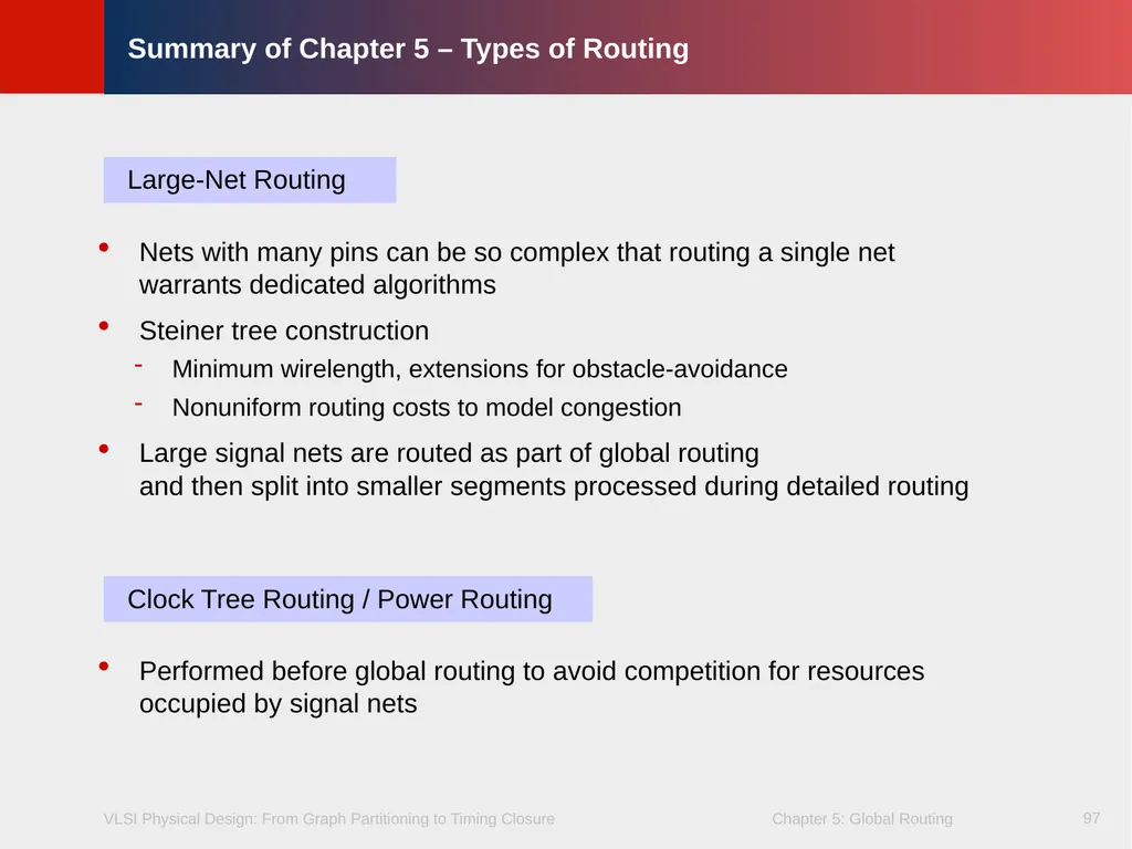
slide97. 97 Summary of Chapter 5 – Types of Routing Nets with many pins can be so complex that routing a single net warrants dedicated algorithms
Steiner tree construction
Minimum wirelength, extensions for obstacle-avoidance
Nonuniform routing costs to model congestion
Large signal nets are routed as part of global routing and then split into smaller segments processed during detailed routing Large-Net Routing Performed before global routing to avoid competition for resources occupied by signal nets Clock Tree Routing / Power Routing<br>
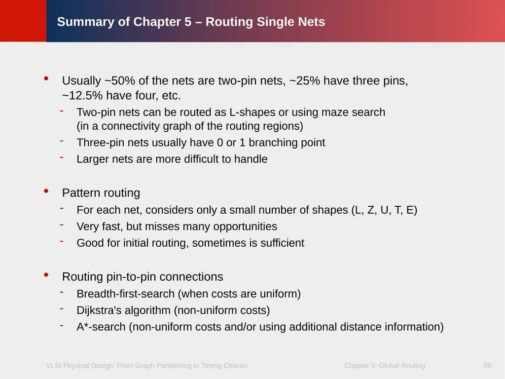
slide98. 98 Summary of Chapter 5 – Routing Single Nets Usually ~50% of the nets are two-pin nets, ~25% have three pins, ~12.5% have four, etc.
Two-pin nets can be routed as L-shapes or using maze search (in a connectivity graph of the routing regions)
Three-pin nets usually have 0 or 1 branching point
Larger nets are more difficult to handle
Pattern routing
For each net, considers only a small number of shapes (L, Z, U, T, E)
Very fast, but misses many opportunities
Good for initial routing, sometimes is sufficient
Routing pin-to-pin connections
Breadth-first-search (when costs are uniform)
Dijkstra's algorithm (non-uniform costs)
A*-search (non-uniform costs and/or using additional distance information)<br>
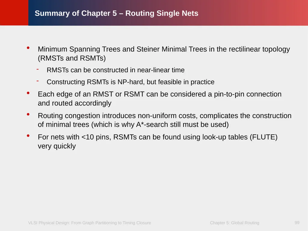
slide99. 99 Summary of Chapter 5 – Routing Single Nets Minimum Spanning Trees and Steiner Minimal Trees in the rectilinear topology (RMSTs and RSMTs)
RMSTs can be constructed in near-linear time
Constructing RSMTs is NP-hard, but feasible in practice
Each edge of an RMST or RSMT can be considered a pin-to-pin connection and routed accordingly
Routing congestion introduces non-uniform costs, complicates the construction of minimal trees (which is why A*-search still must be used)
For nets with <10 pins, RSMTs can be found using look-up tables (FLUTE) very quickly<br>
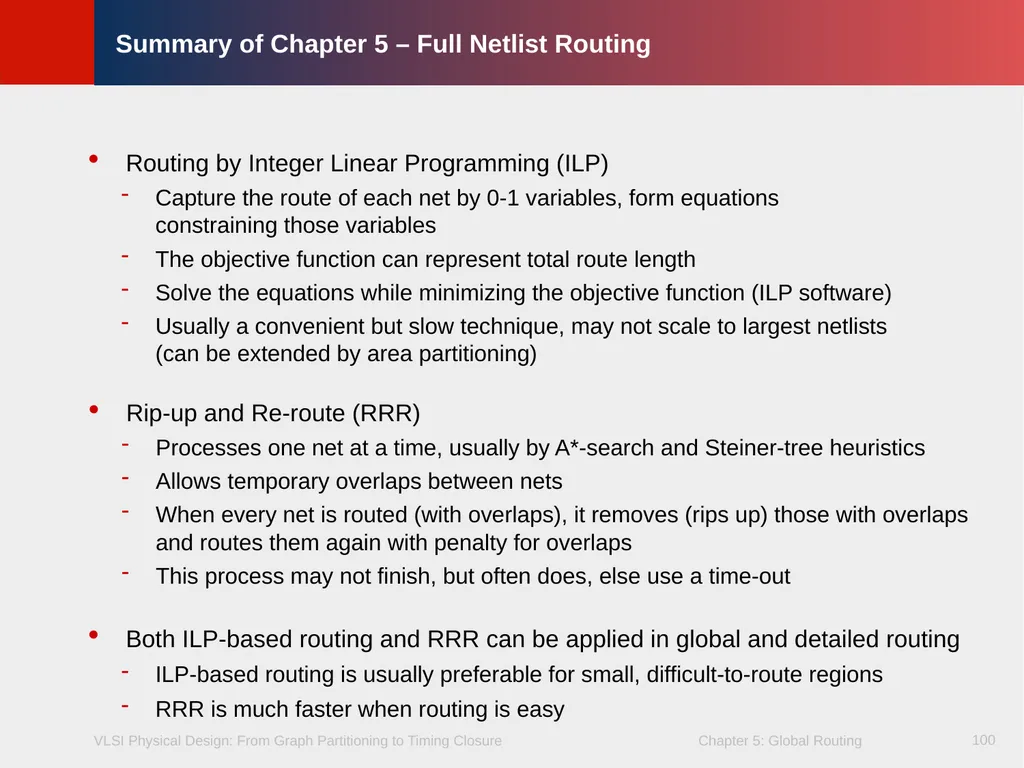
slide100. 100 Summary of Chapter 5 – Full Netlist Routing Routing by Integer Linear Programming (ILP)
Capture the route of each net by 0-1 variables, form equations constraining those variables
The objective function can represent total route length
Solve the equations while minimizing the objective function (ILP software)
Usually a convenient but slow technique, may not scale to largest netlists (can be extended by area partitioning) Rip-up and Re-route (RRR)
Processes one net at a time, usually by A*-search and Steiner-tree heuristics
Allows temporary overlaps between nets
When every net is routed (with overlaps), it removes (rips up) those with overlaps and routes them again with penalty for overlaps
This process may not finish, but often does, else use a time-out Both ILP-based routing and RRR can be applied in global and detailed routing
ILP-based routing is usually preferable for small, difficult-to-route regions
RRR is much faster when routing is easy<br>
slide101. 101 Summary of Chapter 5 – Modern Global Routing Initial routes are constructed quickly by pattern routing and the FLUTE package for Steiner tree construction - very fast
Several iterations based on modified pattern routing to avoid congestion - also very fast
Sometimes completes all routes without violations
If violations remain, they are limited to a few congested spots
The main part of the router is based on a variant of RRR called Negotiated-Congestion Routing (NCR)
Several proposed alternatives are not competitive
NCR maintains "history" in terms of which regions attracted too many nets
NCR increases routing cost according to the historical popularity of the regions
The nets with alternative routes are forced to take those routes
The nets that do not have good alternatives remain unchanged
Speed of increase controls tradeoff between runtime and route quality<br>
slide2. 2 Chapter 5 – Global Routing 5.1 Introduction
5.2 Terminology and Definitions
5.3 Optimization Goals
5.4 Representations of Routing Regions
5.5 The Global Routing Flow
5.6 Single-Net Routing
5.6.1 Rectilinear Routing
5.6.2 Global Routing in a Connectivity Graph
5.6.3 Finding Shortest Paths with Dijkstra’s Algorithm
5.6.4 Finding Shortest Paths with A* Search
5.7 Full-Netlist Routing
5.7.1 Routing by Integer Linear Programming
5.7.2 Rip-Up and Reroute (RRR)
5.8 Modern Global Routing
5.8.1 Pattern Routing
5.8.2 Negotiated-Congestion Routing<br>
slide3. 3 ENTITY test is port a: in bit; end ENTITY test; DRC LVS
ERC Circuit Design Functional Design and Logic Design Physical Design Physical Verification and Signoff Fabrication System Specification Architectural Design Chip Packaging and Testing Chip Planning Placement Signal Routing Partitioning Timing Closure Clock Tree Synthesis 5.1 Introduction © 2022 Springer Verlag<br>
slide4. 4 Given a placement, a netlist and technology information,
determine the necessary wiring, e.g., net topologies and specific routing segments, to connect these cells
while respecting constraints, e.g., design rules and routing resource capacities, and
optimizing routing objectives, e.g., minimizing total wirelength and maximizing timing slack. 5.1 Introduction<br>
slide5. 5 5 Terminology:
Net: Set of two or more pins that have the same electric potential
Netlist: Set of all nets.
Congestion: Where the shortest routes of several nets are incompatible because they traverse the same tracks.
Fixed-die routing: Chip outline and routing resources are fixed.
Variable-die routing: New routing tracks can be added as needed. 5.1 Introduction<br>
slide6. 6 C D A B 4 3 2 1 4 3 4 1 1 6 5 4 Netlist: N1 = {C4, D6, B3}
N2 = {D4, B4, C1, A4}
N3 = {C2, D5}
N4 = {B1, A1, C3} Technology Information (Design Rules) Placement result 5.1 Introduction: General Routing Problem<br>
slide7. 7 Netlist: N1 = {C4, D6, B3}
N2 = {D4, B4, C1, A4}
N3 = {C2, D5}
N4 = {B1, A1, C3} Technology Information (Design Rules) 5.1 Introduction: General Routing Problem C D A B 4 3 2 1 4 3 4 1 1 6 5 4 N1<br>
slide8. 8 Netlist: N1 = {C4, D6, B3}
N2 = {D4, B4, C1, A4}
N3 = {C2, D5}
N4 = {B1, A1, C3} Technology Information (Design Rules) 5.1 Introduction: General Routing Problem C D A B 4 3 2 1 4 3 4 1 1 6 5 4 N2 N3 N4 N1<br>
slide9. 9 Timing-Driven Routing Global Routing Detailed
Routing Large Single- Net Routing Coarse-grain assignment of routes to routing regions (Chap. 5) Fine-grain assignment of routes to routing tracks (Chap. 6) Net topology
optimization
and resource
allocation to
critical nets
(Chap. 8) Power (VDD) and Ground (GND)
routing (Chap. 3) Routing Geometric Techniques Non-Manhattan and clock routing
(Chap. 7) 5.1 Introduction Multi-Stage Routing of Signal Nets<br>
slide10. 10 Wire segments are tentatively assigned (embedded) within the chip layout
Chip area is represented by a coarse routing grid
Available routing resources are represented by edges with capacities in a grid graph
Nets are assigned to these routing resources Global Routing 5.1 Introduction<br>
slide11. 11 Detailed Routing 5.1 Introduction Global Routing<br>
slide12. 12 5.1.2 Globalverdrahtung<br>
slide13. 13 13 5.2 Terminology and Definitions Routing Track: Horizontal wiring path
Routing Column: Vertical wiring path
Routing Region: Region that contains routing tracks or columns
Uniform Routing Region: Evenly spaced horizontal/vertical grid
Non-uniform Routing Region: Horizontal and vertical boundaries that are aligned to external pin connections or macro-cell boundaries resulting in routing regions that have differing sizes<br>
slide14. 14 Channel Standard cell layout (Two-layer routing) 5.2 Terminology and Definitions Rectangular routing region with pins on two opposite sides<br>
slide15. 15 Routing channel Channel Routing channel 5.2 Terminology and Definitions Standard cell layout (Two-layer routing) Rectangular routing region with pins on two opposite sides<br>
slide16. 16 Capacity 5.2 Terminology and Definitions Number of available routing tracks or columns<br>
slide17. 17 For single-layer routing, the capacity is the height h of the channel divided by the pitch dpitch
For multilayer routing, the capacity σ is the sum of the capacities of all layers. Capacity A A B B B B B B C C D C C D dpitch h Horizontal Routing Channel 5.2 Terminology and Definitions Number of available routing tracks or columns<br>
slide18. 18 Horizontal Channel Switchbox (Two-layer macro cell layout) 5.2 Terminology and Definitions Intersection of horizontal and vertical channels Horizontal channel is routed after vertical channel is routed<br>
slide19. 19 T-junction (Two-layer macro cell layout) 5.2 Terminology and Definitions<br>
slide20. 20 2D and 3D Switchboxes Metal5 Bottom pin connection on 3D switchbox 3D switchbox 2D switchbox Pin on channel boundary Top pin connection on cell Horizontal channel Metal4 Metal3 Metal2 Metal1 Vertical channel 5.2 Terminology and Definitions<br>
slide21. 21 Gcells (Tiles) with macro cell layout Metal1 etc. 5.2 Terminology and Definitions<br>
slide22. 22 usw. 5.2 Terminology and Definitions Gcells (Tiles) with standard cells<br>
slide23. 23 Metal1 (Back-to-back- standard cells) etc. 5.2 Terminology and Definitions Gcells (Tiles) with standard cells (back-to-back)<br>
slide24. 24 Global routing seeks to
determine whether a given placement is routable, and
determine a coarse routing for all nets within available routing regions
Considers goals such as
minimizing total wirelength, and
reducing signal delays on critical nets 5.3 Optimization Goals<br>
slide25. 25 5.3 Optimization Goals Full-custom design (2) Channel ordering Layout is dominated by macro cells and routing regions are non-uniform © 2022 Springer Verlag<br>
slide26. 26 5.3 Optimization Goals Standard-cell design A A A A A Feedthrough
cells If number of metal layers is limited, feedthrough cells must be used to route across multiple cell rows Variable-die, standard cell design:
Total height = ΣCell row heights + All channel heights<br>
slide27. 27 5.3 Optimization Goals Standard-cell design Steiner tree solution with minimal wirelength Steiner tree solution with
fewest feedthrough cells<br>
slide28. 28 5.3 Optimization Goals Gate-array design Unrouted net Cell sizes and sizes of routing regions between cells are fixed Key Tasks:
Determine routability
Find a feasible solution<br>
slide29. 29 5.1 Introduction
5.2 Terminology and Definitions
5.3 Optimization Goals
5.4 Representations of Routing Regions
5.5 The Global Routing Flow
5.6 Single-Net Routing
5.6.1 Rectilinear Routing
5.6.2 Global Routing in a Connectivity Graph
5.6.3 Finding Shortest Paths with Dijkstra’s Algorithm
5.6.4 Finding Shortest Paths with A* Search
5.7 Full-Netlist Routing
5.7.1 Routing by Integer Linear Programming
5.7.2 Rip-Up and Reroute (RRR)
5.8 Modern Global Routing
5.8.1 Pattern Routing
5.8.2 Negotiated-Congestion Routing 5.4 Representations of Routing Regions<br>
slide30. 30 Routing regions are represented using efficient data structures
Routing context is captured using a graph, where
nodes represent routing regions and
edges represent adjoining regions
Capacities are associated with both edges and nodes to represent available routing resources 5.4 Representations of Routing Regions<br>
slide31. 31 Grid graph model ggrid = (V,E), where the nodes v V represent the routing grid cells (gcells) and the edges represent connections of grid cell pairs (vi,vj) 5.4 Representations of Routing Regions<br>
slide32. 32 Channel connectivity graph G = (V,E), where the nodes v V represent channels, and the edges E represent adjacencies of the channels 5.4 Representations of Routing Regions<br>
slide33. 33 Switchbox connectivity graph G = (V, E), where the nodes v V represent switchboxes and an edge exists between two nodes if the corresponding switchboxes are on opposite sides of the same channel 5.4 Representations of Routing Regions<br>
slide34. 34 5.5 The Global Routing Flow – General Idea Defining the routing regions (Region definition)
Layout area is divided into routing regions
Nets can also be routed over standard cells
Regions, capacities and connections are represented by a graph
Mapping nets to the routing regions (Region assignment)
Each net of the design is assigned to one or several routing regions to connect all of its pins
Routing capacity, timing and congestion affect mapping
Assigning crosspoints along the edges of the routing regions (Midway routing)
Routes are assigned to fixed locations or crosspoints along the edges of the routing regions
Enables scaling of global and detailed routing<br>
slide35. 35 5.1 Introduction
5.2 Terminology and Definitions
5.3 Optimization Goals
5.4 Representations of Routing Regions
5.5 The Global Routing Flow
5.6 Single-Net Routing
5.6.1 Rectilinear Routing
5.6.2 Global Routing in a Connectivity Graph
5.6.3 Finding Shortest Paths with Dijkstra’s Algorithm
5.6.4 Finding Shortest Paths with A* Search
5.7 Full-Netlist Routing
5.7.1 Routing by Integer Linear Programming
5.7.2 Rip-Up and Reroute (RRR)
5.8 Modern Global Routing
5.8.1 Pattern Routing
5.8.2 Negotiated-Congestion Routing 5.6 Single-Net Routing<br>
slide36. 36 B (2, 6) A (2, 1) C (6, 4) B (2, 6) A (2, 1) C (6, 4) S (2, 4) Rectilinear Steiner minimum tree (RSMT) Rectilinear minimum spanning tree (RMST) 5.6.1 Rectilinear Routing<br>
slide37. 37 37 5.6.1 Rectilinear Routing An RMST can be computed in O(p2) time, where p is the number of terminals in the net using methods such as Prim’s Algorithm
Prim’s Algorithm builds an MST by starting with a single terminal and greedily adding least-cost edges to the partially-constructed tree
Advanced computational-geometric techniques reduce the runtime to O(p log p)<br>
slide38. 38 Characteristics of an RSMT
An RSMT for a p-pin net has between 0 and p – 2 (inclusive) Steiner points
The degree of any terminal pin is 1, 2, 3, or 4 The degree of a Steiner point is either 3 or 4
A RSMT is always enclosed in the minimum bounding box (MBB) of the net
The total edge length LRSMT of the RSMT is at least half the perimeter
of the minimum bounding box of the net: LRSMT LMBB / 2 5.6.1 Rectilinear Routing<br>
slide39. 39 Transforming an initial RMST into a low-cost RSMT 5.6.1 Rectilinear Routing © 2022 Springer Verlag<br>
slide40. 40 Hanan grid
Adding Steiner points to an RMST can significantly reduce the wirelength
Maurice Hanan proved that for finding Steiner points, it suffices to consider only points located at the intersections of vertical and horizontal lines that pass through terminal pins
The Hanan grid consists of the lines x = xp, y = yp that pass through the location (xp,yp) of each terminal pin p
The Hanan grid contains at most (n2-n) candidate Steiner points (n = number of pins), thereby greatly reducing the solution space for finding an RSMT 5.6.1 Rectilinear Routing<br>
slide41. 41 5.6.1 Rectilinear Routing © 2022 Springer Verlag<br>
slide42. 42 5.6.1 Rectilinear Routing<br>
slide43. 43 Sequential Steiner Tree Heuristic 5.6.1 Rectilinear Routing<br>
slide44. 44 A Sequential Steiner Tree Heuristic
Find the closest (in terms of rectilinear distance) pin pair, construct their minimum bounding box (MBB)
Find the closest point pair (pMBB,pC) between any point pMBB on the MBB and pC from the set of pins to consider
Construct the MBB of pMBB and pC
Add the L-shape that pMBB lies on to T (deleting the other L-shape). If pMBB is a pin, then add any L-shape of the MBB to T.
Goto step 2 until the set of pins to consider is empty 5.6.1 Rectilinear Routing<br>
slide45. 45 1 5.6.1 Rectilinear Routing: Example Sequential Steiner Tree Heuristic<br>
slide46. 46 1 2 1 5.6.1 Rectilinear Routing: Example Sequential Steiner Tree Heuristic<br>
slide47. 47 1 2 3 1 5.6.1 Rectilinear Routing: Example Sequential Steiner Tree Heuristic MBB pc<br>
slide48. 48 1 2 3 1 2 3 1 2 4 5.6.1 Rectilinear Routing: Example Sequential Steiner Tree Heuristic pMBB<br>
slide49. 49 1 2 3 1 2 3 4 5 1 2 3 4 1 2 3 5.6.1 Rectilinear Routing: Example Sequential Steiner Tree Heuristic<br>
slide50. 50 1 2 3 1 2 3 4 5 1 2 3 4 1 2 3 4 5 6 1 2 3 4 5.6.1 Rectilinear Routing: Example Sequential Steiner Tree Heuristic<br>
slide51. 51 1 2 3 4 5 6 7 1 2 3 1 2 3 4 5 1 2 3 4 1 2 3 4 5 6 1 2 3 4 5 5.6.1 Rectilinear Routing: Example Sequential Steiner Tree Heuristic<br>
slide52. 52 1 2 3 4 5 6 7 1 2 3 1 2 3 4 5 1 2 3 4 5 6 7 1 2 3 4 1 2 3 4 5 6 1 2 3 4 5 6 5.6.1 Rectilinear Routing: Example Sequential Steiner Tree Heuristic © 2022 Springer Verlag<br>
slide53. 53 1 2 3 4 5 6 7 1 2 3 1 2 3 4 5 1 2 3 4 5 6 7 1 2 3 4 1 2 3 4 5 6 1 2 3 4 5 6 5.6.1 Rectilinear Routing: Example Sequential Steiner Tree Heuristic © 2022 Springer Verlag<br>
slide54. 54 1 2 3 4 5 6 7 8 9 1 2 3 4 5 6 7 8 9 10 11 12 13 14 Channel connectivity graph Switchbox connectivity graph 5.6.2 Global Routing in a Connectivity Graph<br>
slide55. 55 5.6.2 Global Routing in a Connectivity Graph Channel connectivity graph Switchbox connectivity graph<br>
slide56. 56 Combines switchboxes and channels, handles non-rectangular block shapes
Suitable for full-custom design and multi-chip modules
Overview: 5.6.2 Global Routing in a Connectivity Graph © 2022 Springer Verlag<br>
slide57. 57 Horizontal macro-cell edges Vertical macro-cell edges Defining the routing regions 5.6.2 Global Routing in a Connectivity Graph +<br>
slide58. 58 2 3 4 5 6 7 8 9 10 11 12 13 14 15 16 17 18 19 20 21 22 23 24 25 26 27 1 2 3 4 5 6 7 8 9 10 11 12 13 14 15 16 17 18 19 20 21 22 23 24 25 26 27 1 Defining the connectivity graph 5.6.2 Global Routing in a Connectivity Graph<br>
slide59. 59 2 3 4 5 6 7 8 9 10 11 12 13 14 15 16 17 18 19 20 21 22 23 24 25 26 27 1 2 3 4 5 6 7 8 9 10 11 12 13 14 15 16 17 18 19 20 21 22 23 24 25 26 27 1,2 Horizontal capacity of routing region 1 Vertical capacity of routing region 1 2 Tracks 1 Track 1 5.6.2 Global Routing in a Connectivity Graph<br>
slide60. 60 2 3 4 5 6 7 8 9 10 11 12 13 14 15 16 17 18 19 20 21 22 23 24 25 26 27 1 2 3 4 5 6 7 8 9 10 11 12 13 14 15 16 17 18 19 20 21 22 23 24 25 26 27 1,2 2,2 2,2 2,2 3,2 1,2 1,2 2,1 3,1 1,3 2,3 1,1 2,1 3,1 3,1 1,1 2,1 4,1 3,1 1,1 6,1 3,1 1,1 1,1 1,4 3,4 1,8 1 5.6.2 Global Routing in a Connectivity Graph<br>
slide61. 61 Algorithm Overview
Define routing regions
Define connectivity graph
Determine net ordering
Assign tracks for all pin connections in Netlist
Consider each net
Free corresponding tracks for net’s pins
Decompose net into two-pin subnets
Find shortest path for subnet connectivity graph
If no shortest path exists, do not route, otherwise, assign subnet to the nodes of shortest path and update routing capacities
If there are unrouted nets, goto Step 5, otherwise END 5.6.2 Global Routing in a Connectivity Graph<br>
slide62. 62 l 1 2 3 4 5 6 7 8 9 10 11 12 B A B A w Example
Global routing of the nets A-A and B-B<br>
slide63. 63 l 1 2 3 4 5 6 7 8 9 10 11 12 B A B A w 1 2 3 4 2,2 4,2 1,2 2,7 4,2 1,2 1,2 5 6 8 4,2 7 2,2 4,2 9 10 4,2 1,5 11 12 B A B A 0,1 3,1 0,4 Example
Global routing of the nets A-A and B-B<br>
slide64. 64 l 1 2 3 4 5 6 7 8 9 10 11 12 B A B A w 1 2 3 4 2,2 4,2 1,2 2,7 4,2 1,2 1,2 5 6 8 4,2 7 2,2 4,2 9 10 4,2 1,5 11 12 B A B A B A B A 1 2 3 4 2,2 4,2 1,2 2,7 4,2 0,1 1,2 5 6 8 3,1 7 2,2 4,2 9 10 4,2 0,4 11 12 Example
Global routing of the nets A-A and B-B © 2022 Springer Verlag<br>
slide65. 65 l 1 2 3 4 5 6 7 8 9 10 11 12 B A B A w B A B A Example
Global routing of the nets A-A and B-B<br>
slide66. 66 B A B A 4 5 7 8 6 9 10 1 2 3 Example
Determine routability of a placement ?<br>
slide67. 67 B A B A 4 5 7 8 6 9 10 1 2 3 B A B A 4 5 7 8 6 9 10 1 2 3 B A B A 4 5 7 8 6 9 10 1 2 3 1 2 3 3,1 3,4 3,3 0,3 0,1 0,4 0,2 3,4 3,1 2,2 4 5 6 7 8 9 10 1 2 3 2,0 2,3 3,3 0,2 0,0 0,3 0,2 2,3 2,0 2,2 4 5 6 7 8 9 10 Example
Determine routability of a placement<br>
slide68. 68 B A B A 4 5 7 8 6 9 10 1 2 3 B A B A 4 5 7 8 6 9 10 1 2 3 Example
Determine routability of a placement<br>
slide69. 69 Finds a shortest path between two specific nodes in the routing graph
Input
graph G(V,E) with non-negative edge weights W,
source (starting) node s, and
target (ending) node t
Maintains three groups of nodes
Group 1 – contains the nodes that have not yet been visited
Group 2 – contains the nodes that have been visited but for which the shortest-path cost from the starting node has not yet been found
Group 3 – contains the nodes that have been visited and for which the shortest path cost from the starting node has been found
Once t is in Group 3, the algorithm finds the shortest path by backtracing 5.6.3 Finding Shortest Paths with Dijkstra’s Algorithm<br>
slide70. 70 1 4 7 2 5 8 3 6 9 s t 1,4 8,8 2,6 2,8 9,8 3,3 8,6 9,7 3,2 1,4 2,8 4,5 Find the shortest path from source s to target t where the path cost ∑w1 + ∑w2 is minimal 5.6.3 Finding Shortest Paths with Dijkstra’s Algorithm Example<br>
slide71. 71 1 4 7 2 5 8 3 6 9 s t 1,4 8,8 2,6 2,8 9,8 3,3 8,6 9,7 3,2 1,4 2,8 4,5 (1) Current node: 1<br>
slide72. 72 [1] N [2] 8,6 W [4] 1,4 W [4] 1,4 parent of node [node name] ∑w1(s,node),∑w2(s,node) 1 4 7 2 5 8 3 6 9 1,4 8,8 2,6 2,8 9,8 3,3 8,6 9,7 3,2 1,4 2,8 4,5 Current node: 1 Neighboring nodes: 2, 4 Minimum cost in group 2: node 4 s t<br>
slide73. 73 1 4 7 2 5 8 3 6 9 1,4 8,8 2,6 2,8 9,8 3,3 8,6 9,7 3,2 1,4 2,8 4,5 [1] N [2] 8,6 W [4] 1,4 W [4] 1,4 N [5] 10,11 W [7] 9,12 N [2] 8,6 Current node: 4
Neighboring nodes: 1, 5, 7 Minimum cost in group 2: node 2 s t parent of node [node name] ∑w1(s,node),∑w2(s,node)<br>
slide74. 74 1 4 7 2 5 8 3 6 9 1,4 8,8 2,6 2,8 9,8 3,3 8,6 9,7 3,2 1,4 2,8 4,5 [1] N [2] 8,6 W [4] 1,4 W [4] 1,4 N [5] 10,11 W [7] 9,12 N [2] 8,6 N [3] 9,10 W [5] 10,12 N [3] 9,10 Current node: 2
Neighboring nodes: 1, 3, 5 Minimum cost in group 2: node 3 s t parent of node [node name] ∑w1(s,node),∑w2(s,node)<br>
slide75. 75 1 4 7 2 5 8 3 6 9 1,4 8,8 2,6 2,8 9,8 3,3 8,6 9,7 3,2 1,4 2,8 4,5 [1] N [2] 8,6 W [4] 1,4 W [4] 1,4 N [5] 10,11 W [7] 9,12 N [2] 8,6 N [3] 9,10 W [5] 10,12 N [3] 9,10 W [6] 18,18 N [5] 10,11 Current node: 3
Neighboring nodes: 2, 6 Minimum cost in group 2: node 5 s t parent of node [node name] ∑w1(s,node),∑w2(s,node)<br>
slide76. 76 1 4 7 2 5 8 3 6 9 1,4 8,8 2,6 2,8 9,8 3,3 8,6 9,7 3,2 1,4 2,8 4,5 [1] N [2] 8,6 W [4] 1,4 W [4] 1,4 N [5] 10,11 W [7] 9,12 N [2] 8,6 N [3] 9,10 W [5] 10,12 N [3] 9,10 W [6] 18,18 N [5] 10,11 N [6] 12,19 W [8] 12,19 W [7] 9,12 Current node: 5
Neighboring nodes: 2, 4, 6, 8 Minimum cost in group 2: node 7 s t parent of node [node name] ∑w1(s,node),∑w2(s,node)<br>
slide77. 77 1 4 7 2 5 8 3 6 9 1,4 8,8 2,6 2,8 9,8 3,3 8,6 9,7 3,2 1,4 2,8 4,5 (1) N (2) 8,6 W (4) 1,4 W (4) 1,4 N (5) 10,11 W (7) 9,12 N (2) 8,6 N (3) 9,10 W (5) 10,12 N (3) 9,10 W (6) 18,18 N (5) 10,11 N (6) 12,19 W (8) 12,19 W (7) 9,12 N (8) 12,14 N (8) 12,14 Current node: 7
Neighboring nodes: 4, 8 Minimum cost in group 2: node 8 s t parent of node [node name] ∑w1(s,node),∑w2(s,node)<br>
slide78. 78 1 7 2 5 8 3 6 9 1,4 8,8 2,6 2,8 9,8 3,3 8,6 9,7 3,2 1,4 2,8 4,5 (1) N (2) 8,6 W (4) 1,4 W (4) 1,4 N (5) 10,11 W (7) 9,12 N (2) 8,6 N (3) 9,10 W (5) 10,12 N (3) 9,10 W (6) 18,18 N (5) 10,11 N (6) 12,19 W (8) 12,19 W (7) 9,12 N (8) 12,14 N (8) 12,14 Retrace from t to s s t 4<br>
slide79. 79 1 4 7 2 5 8 3 6 9 1,4 9,12 12,14 Optimal path 1-4-7-8 from s to t with accumulated cost (12,14) s t<br>
slide80. 80 5.6.4 Finding Shortest Paths with A* Search A* search operates similarly to Dijkstra’s algorithm, but extends the cost function to include an estimated distance from the current node to the target
Expands only the most promising nodes; its best-first search strategy eliminates a large portion of the solution space<br>
slide81. 81 5.6.4 Finding Shortest Paths with A* Search Bidirectional A* search: nodes are expanded from both the source and target until the two expansion regions intersect
Number of nodes considered can be reduced<br>
slide82. 82 5.1 Introduction
5.2 Terminology and Definitions
5.3 Optimization Goals
5.4 Representations of Routing Regions
5.5 The Global Routing Flow
5.6 Single-Net Routing
5.6.1 Rectilinear Routing
5.6.2 Global Routing in a Connectivity Graph
5.6.3 Finding Shortest Paths with Dijkstra’s Algorithm
5.6.4 Finding Shortest Paths with A* Search
5.7 Full-Netlist Routing
5.7.1 Routing by Integer Linear Programming
5.7.2 Rip-Up and Reroute (RRR)
5.8 Modern Global Routing
5.8.1 Pattern Routing
5.8.2 Negotiated-Congestion Routing 5.7 Full-Netlist Routing<br>
slide83. 83 5.7 Full-Netlist Routing Global routers must properly match nets with routing resources, without oversubscribing resources in any part of the chip
Signal nets are either routed
simultaneously, e.g., by integer linear programming, or
sequentially, e.g., one net at a time
When certain nets cause resource contention or overflow for routing edges, sequential routing requires multiple iterations: rip-up and reroute<br>
slide84. 84 5.7.1 Routing by Integer Linear Programming A linear program (LP) consists
of a set of constraints and
an optional objective function
Objective function is maximized or minimized
Both the constraints and the objective function must be linear
Constraints form a system of linear equations and inequalities
Integer linear program (ILP): linear program where every variable can only assume integer values
Typically takes much longer to solve
In many cases, variables are only allowed values 0 and 1
Several ways to formulate the global routing problem as an ILP, one of which is presented next<br>
slide85. 85 5.7.1 Routing by Integer Linear Programming Three inputs
W × H routing grid G,
Routing edge capacities, and
Netlist
Two sets of variables
k Boolean variables xnet1, xnet2, … , xnetk, each of which serves as an indicator for one of k specific paths or route options, for each net net Netlist
k real variables wnet1, wnet2, … , wnetk, each of which represents a net weight for a specific route option for net Netlist
Two types of constraints
Each net must select a single route (mutual exclusion)
Number of routes assigned to each edge (total usage) cannot exceed its capacity<br>
slide86. 86 5.7.1 Routing by Integer Linear Programming Inputs
W,H: width W and height H of routing grid G
G(i,j): grid cell at location (i,j) in routing grid G
σ(G(i,j)~G(i + 1,j)): capacity of horizontal edge G(i,j) ~ G(i + 1,j)
σ(G(i,j)~G(i,j + 1)): capacity of vertical edge G(i,j) ~ G(i,j + 1)
Netlist: netlist
Variables
xnet1, ... , xnetk: k Boolean path variables for each net net Netlist
wnet1, ... , wnetk: k net weights, one for each path of net net Netlist
Maximize
Subject to
Variable ranges
Net constraints
Capacity constraints<br>
slide87. 87 5.7.1 Routing by Integer Linear Programming – Example Global Routing Using Integer Linear Programming
Given
Nets A, B
W = 5 × H = 4 routing grid G
σ(e) = 1 for all e G
L-shapes have weight 1.00 and Z-shapes have weight 0.99
The lower-left corner is (0,0).
Task
Write the ILP to route the nets in the graph below<br>
slide88. 88 5.7.1 Routing by Integer Linear Programming – Example Solution
For net A, the possible routes are two L-shapes (A1,A2) and two Z-shapes (A3,A4)
For net B, the possible routes are two L-shapes (B1,B2) and one Z-shape (B3)
For net C, the possible routes are two L-shapes (C1,C2) and two Z-shapes (C3,C4)<br>
slide89. 89 5.7.1 Routing by Integer Linear Programming – Example Horizontal Edge Capacity Constraints:
G(0,0) ~ G(1,0): xC1 + xC3 ≤ σ(G(0,0) ~ G(1,0)) = 1
G(1,0) ~ G(2,0): xC1 ≤ σ(G(1,0) ~ G(2,0)) = 1
G(2,0) ~ G(3,0): xB1 + xB3 ≤ σ(G(2,0) ~ G(3,0)) = 1
G(3,0) ~ G(4,0): xB1 ≤ σ(G(3,0) ~ G(4,0)) = 1
G(0,1) ~ G(1,1): xA2 + xC4 ≤ σ(G(0,1) ~ G(1,1)) = 1
G(1,1) ~ G(2,1): xA2 + xA3 + xC4 ≤ σ(G(1,1) ~ G(2,1)) = 1
G(2,1) ~ G(3,1): xB2 ≤ σ(G(2,1) ~ G(3,1)) = 1
G(3,1) ~ G(4,1): xB2 + xB3 ≤ σ(G(3,1) ~ G(4,1)) = 1
G(0,2) ~ G(1,2): xA4 + xC2 ≤ σ(G(0,2) ~ G(1,2)) = 1
G(1,2) ~ G(2,2): xA4 + xC2 + xC3 ≤ σ(G(1,2) ~ G(2,2)) = 1
G(0,3) ~ G(1,3): xA1 + xA3 ≤ σ(G(0,3) ~ G(1,3)) = 1
G(1,3) ~ G(2,3): xA1 ≤ σ(G(1,3) ~ G(2,3)) = 1 Vertical Edge Capacity Constraints:
G(0,0) ~ G(0,1): xC2 + xC4 ≤ σ(G(0,0) ~ G(0,1)) = 1
G(1,0) ~ G(1,1): xC3 ≤ σ(G(1,0) ~ G(1,1)) = 1
G(2,0) ~ G(2,1): xB2 + xC1 ≤ σ(G(2,0) ~ G(2,1)) = 1
G(3,0) ~ G(3,1): xB3 ≤ σ(G(3,0) ~ G(3,1)) = 1
G(4,0) ~ G(4,1): xB1 ≤ σ(G(4,0) ~ G(4,1)) = 1
G(0,1) ~ G(0,2): xA2 + xC2 ≤ σ(G(0,1) ~ G(0,2)) = 1
G(1,1) ~ G(1,2): xA3 + xC3 ≤ σ(G(1,1) ~ G(1,2)) = 1
G(2,1) ~ G(2,2): xA1 + xA4 + xC1 + xC4 ≤ σ(G(2,1) ~ G(2,2)) = 1
G(0,2) ~ G(0,3): xA2 + xA4 ≤ σ(G(0,2) ~ G(0,3)) = 1
G(1,2) ~ G(1,3): xA3 ≤ σ(G(1,2) ~ G(1,3)) = 1
G(2,2) ~ G(2,3): xA1 ≤ σ(G(2,2) ~ G(2,3)) = 1<br>
slide90. 90 5.7.2 Rip-Up and Reroute (RRR) Rip-up and reroute (RRR) framework: focuses on hard-to-route nets
Idea: allow temporary violations, so that all nets are routed, but then iteratively remove some nets (rip-up), and route them differently (reroute)<br>
slide91. 91 5.1 Introduction
5.2 Terminology and Definitions
5.3 Optimization Goals
5.4 Representations of Routing Regions
5.5 The Global Routing Flow
5.6 Single-Net Routing
5.6.1 Rectilinear Routing
5.6.2 Global Routing in a Connectivity Graph
5.6.3 Finding Shortest Paths with Dijkstra’s Algorithm
5.6.4 Finding Shortest Paths with A* Search
5.7 Full-Netlist Routing
5.7.1 Routing by Integer Linear Programming
5.7.2 Rip-Up and Reroute (RRR)
5.8 Modern Global Routing
5.8.1 Pattern Routing
5.8.2 Negotiated-Congestion Routing 5.8 Modern Global Routing<br>
slide92. 92 General flow for modern global routers, where each router uses a unique set of optimizations: 5.8 Modern Global Routing<br>
slide93. 93 Pattern Routing
Searches through a small number of route patterns to improve runtime
Topologies commonly used in pattern routing: L-shapes, Z-shapes, U-shapes 5.8 Modern Global Routing<br>
slide94. 94 Negotiated-Congestion Routing
Each edge e is assigned a cost value cost(e) that reflects the demand for edge e
A segment from net net that is routed through e pays a cost of cost(e)
Total cost of net is the sum of cost(e) values taken over all edges used by net:
The edge cost cost(e) is increased according to the edge congestion φ(e), defined as the total number of nets passing through e divided by the capacity of e:
A higher cost(e) value discourages nets from using e and implicitly encourages nets to seek out other, less used edges
Iterative routing approaches (Dijkstra’s algorithm, A* search, etc.) find routes with minimum cost while respecting edge capacities 5.8 Modern Global Routing<br>
slide95. 95 Summary of Chapter 5 – Types of Routing Input: netlist, placement, obstacles + (usually) routing grid
Partitions the routing region (chip or block) into global routing cells (gcells)
Considers the locations of cells within a region as identical
Plans routes as sequences of gcells
Minimizes total length of routes and, possibly, routed congestion
May fail if routing resources are insufficient
Variable-die can expand the routing area, so can't usually fail
Fixed-die is more common today (cannot resize a block in a larger chip)
Interpreting failures in global routing
Failure with many violations => must restructure the netlist and/or redo global placement
Failure with few violations => detailed routing may be able to fix the problems Global Routing<br>
slide96. 96 Summary of Chapter 5 – Types of Routing Input: netlist, placement, obstacles, global routes (on a routing grid), routing tracks, design rules
Seeks to implement each global route as a sequence of track segments
Includes layer assignment (unless that is performed during global routing)
Minimizes total length of routes, subject to design rules Detailed Routing Minimizes circuit delay by optimizing timing-critical nets
Usually needs to trade off route length and congestion against timing
Both global and detailed routing can be timing-driven Timing-Driven routing<br>
slide97. 97 Summary of Chapter 5 – Types of Routing Nets with many pins can be so complex that routing a single net warrants dedicated algorithms
Steiner tree construction
Minimum wirelength, extensions for obstacle-avoidance
Nonuniform routing costs to model congestion
Large signal nets are routed as part of global routing and then split into smaller segments processed during detailed routing Large-Net Routing Performed before global routing to avoid competition for resources occupied by signal nets Clock Tree Routing / Power Routing<br>
slide98. 98 Summary of Chapter 5 – Routing Single Nets Usually ~50% of the nets are two-pin nets, ~25% have three pins, ~12.5% have four, etc.
Two-pin nets can be routed as L-shapes or using maze search (in a connectivity graph of the routing regions)
Three-pin nets usually have 0 or 1 branching point
Larger nets are more difficult to handle
Pattern routing
For each net, considers only a small number of shapes (L, Z, U, T, E)
Very fast, but misses many opportunities
Good for initial routing, sometimes is sufficient
Routing pin-to-pin connections
Breadth-first-search (when costs are uniform)
Dijkstra's algorithm (non-uniform costs)
A*-search (non-uniform costs and/or using additional distance information)<br>
slide99. 99 Summary of Chapter 5 – Routing Single Nets Minimum Spanning Trees and Steiner Minimal Trees in the rectilinear topology (RMSTs and RSMTs)
RMSTs can be constructed in near-linear time
Constructing RSMTs is NP-hard, but feasible in practice
Each edge of an RMST or RSMT can be considered a pin-to-pin connection and routed accordingly
Routing congestion introduces non-uniform costs, complicates the construction of minimal trees (which is why A*-search still must be used)
For nets with <10 pins, RSMTs can be found using look-up tables (FLUTE) very quickly<br>
slide100. 100 Summary of Chapter 5 – Full Netlist Routing Routing by Integer Linear Programming (ILP)
Capture the route of each net by 0-1 variables, form equations constraining those variables
The objective function can represent total route length
Solve the equations while minimizing the objective function (ILP software)
Usually a convenient but slow technique, may not scale to largest netlists (can be extended by area partitioning) Rip-up and Re-route (RRR)
Processes one net at a time, usually by A*-search and Steiner-tree heuristics
Allows temporary overlaps between nets
When every net is routed (with overlaps), it removes (rips up) those with overlaps and routes them again with penalty for overlaps
This process may not finish, but often does, else use a time-out Both ILP-based routing and RRR can be applied in global and detailed routing
ILP-based routing is usually preferable for small, difficult-to-route regions
RRR is much faster when routing is easy<br>
slide101. 101 Summary of Chapter 5 – Modern Global Routing Initial routes are constructed quickly by pattern routing and the FLUTE package for Steiner tree construction - very fast
Several iterations based on modified pattern routing to avoid congestion - also very fast
Sometimes completes all routes without violations
If violations remain, they are limited to a few congested spots
The main part of the router is based on a variant of RRR called Negotiated-Congestion Routing (NCR)
Several proposed alternatives are not competitive
NCR maintains "history" in terms of which regions attracted too many nets
NCR increases routing cost according to the historical popularity of the regions
The nets with alternative routes are forced to take those routes
The nets that do not have good alternatives remain unchanged
Speed of increase controls tradeoff between runtime and route quality<br>