
Comparing Two Means Prof. Andy Field Aims t-tests:
Description: Comparing Two Means Prof. Andy Field Aims t-tests: Independent Dependent (aka paired, matched) Rationale for the tests Assumptions t-tests as a GLM Interpretation Calculating an effect size Reporting results Robust methods Experiments The
Related Topics
Download Presentation
"Comparing Two Means Prof. Andy Field Aims t-tests:" is the property of its rightful owner. Permission is granted to download and print the materials on this website for personal, non-commercial use only, and to display it on your personal computer provided you do not modify the materials and that you retain all copyright notices contained in the materials. By downloading content from our website, you accept the terms of this agreement.
Presentation Transcript
slide1. Comparing Two Means Prof. Andy Field<br>
slide2. Aims t-tests:
Independent
Dependent (aka paired, matched)
Rationale for the tests
Assumptions
t-tests as a GLM
Interpretation
Calculating an effect size
Reporting results
Robust methods<br>
slide3. Experiments The simplest form of experiment that can be done is one with only one independent variable that is manipulated in only two ways and only one outcome is measured.
More often than not, the manipulation of the independent variable involves having an experimental condition and a control.
E.g., Is the movie Scream 2 scarier than the original Scream? We could measure heart rates (which indicate anxiety) during both films and compare them.
This situation can be analysed with a t-test<br>
slide4. t-test Independent t-test
Compares two means based on independent data.
E.g., data from different groups of people.
Dependent t-test
Compares two means based on related data.
E.g., Data from the same people measured at different times.
Data from ‘matched’ samples.
Significance testing
Testing the significance of Pearson’s correlation coefficient
Testing the significance of b in regression.<br>
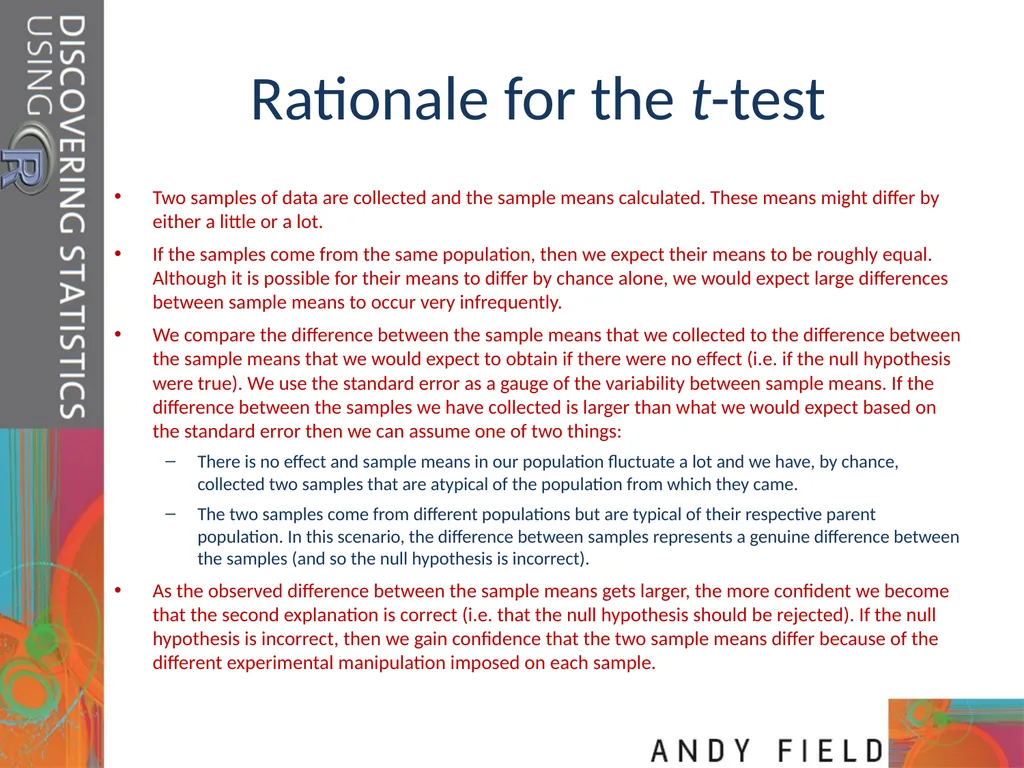
slide5. Rationale for the t-test Two samples of data are collected and the sample means calculated. These means might differ by either a little or a lot.
If the samples come from the same population, then we expect their means to be roughly equal. Although it is possible for their means to differ by chance alone, we would expect large differences between sample means to occur very infrequently.
We compare the difference between the sample means that we collected to the difference between the sample means that we would expect to obtain if there were no effect (i.e. if the null hypothesis were true). We use the standard error as a gauge of the variability between sample means. If the difference between the samples we have collected is larger than what we would expect based on the standard error then we can assume one of two things:
There is no effect and sample means in our population fluctuate a lot and we have, by chance, collected two samples that are atypical of the population from which they came.
The two samples come from different populations but are typical of their respective parent population. In this scenario, the difference between samples represents a genuine difference between the samples (and so the null hypothesis is incorrect).
As the observed difference between the sample means gets larger, the more confident we become that the second explanation is correct (i.e. that the null hypothesis should be rejected). If the null hypothesis is incorrect, then we gain confidence that the two sample means differ because of the different experimental manipulation imposed on each sample.<br>
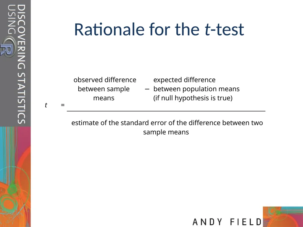
slide6. Rationale for the t-test<br>
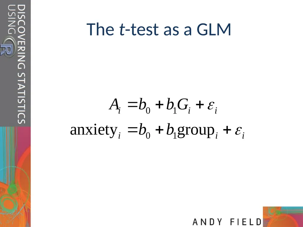
slide7. The t-test as a GLM<br>
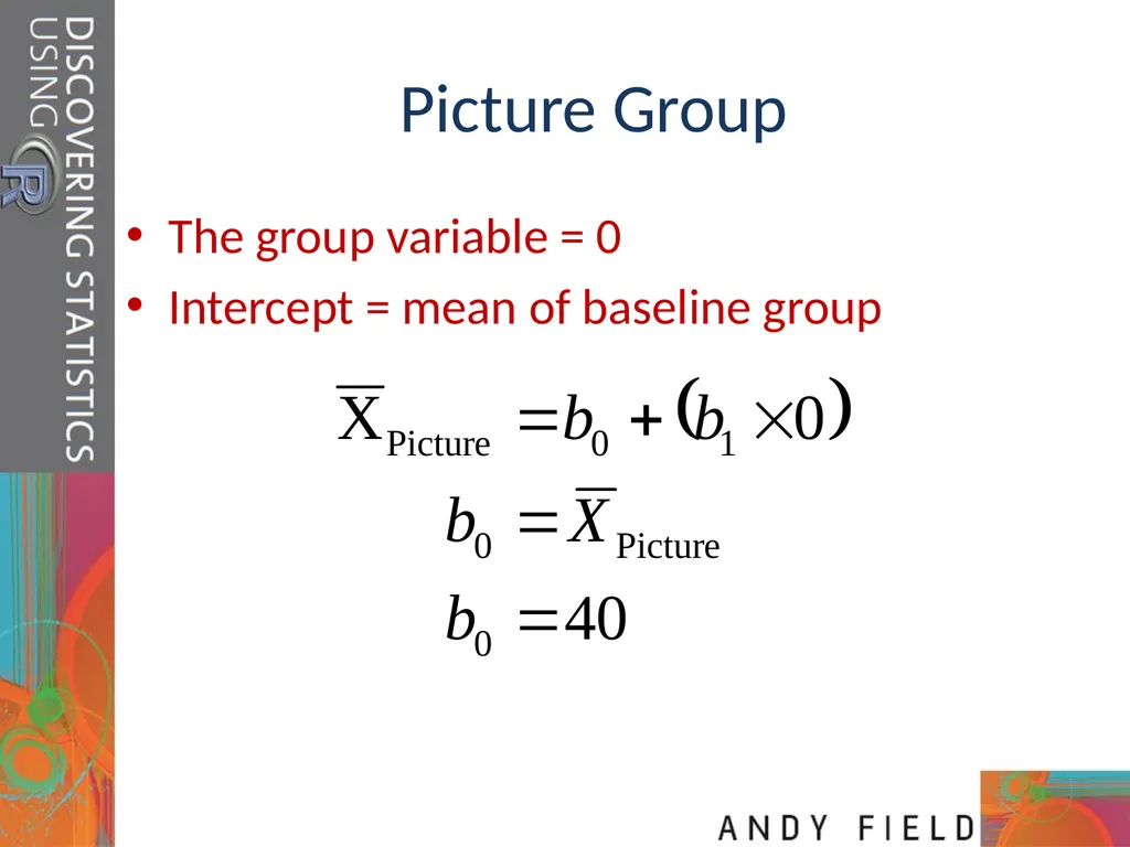
slide8. Picture Group The group variable = 0
Intercept = mean of baseline group<br>
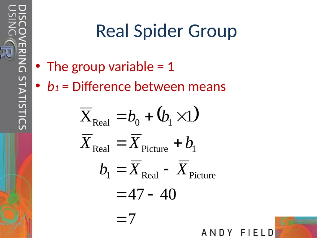
slide9. Real Spider Group The group variable = 1
b1 = Difference between means<br>
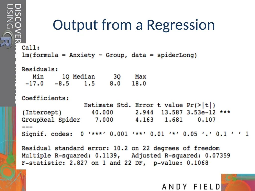
slide10. Output from a Regression<br>
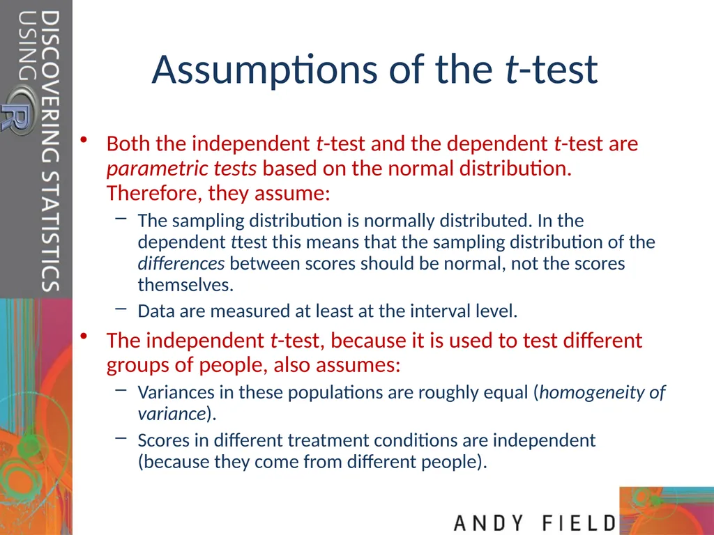
slide11. Assumptions of the t-test Both the independent t-test and the dependent t-test are parametric tests based on the normal distribution. Therefore, they assume:
The sampling distribution is normally distributed. In the dependent ttest this means that the sampling distribution of the differences between scores should be normal, not the scores themselves.
Data are measured at least at the interval level.
The independent t-test, because it is used to test different groups of people, also assumes:
Variances in these populations are roughly equal (homogeneity of variance).
Scores in different treatment conditions are independent (because they come from different people).<br>
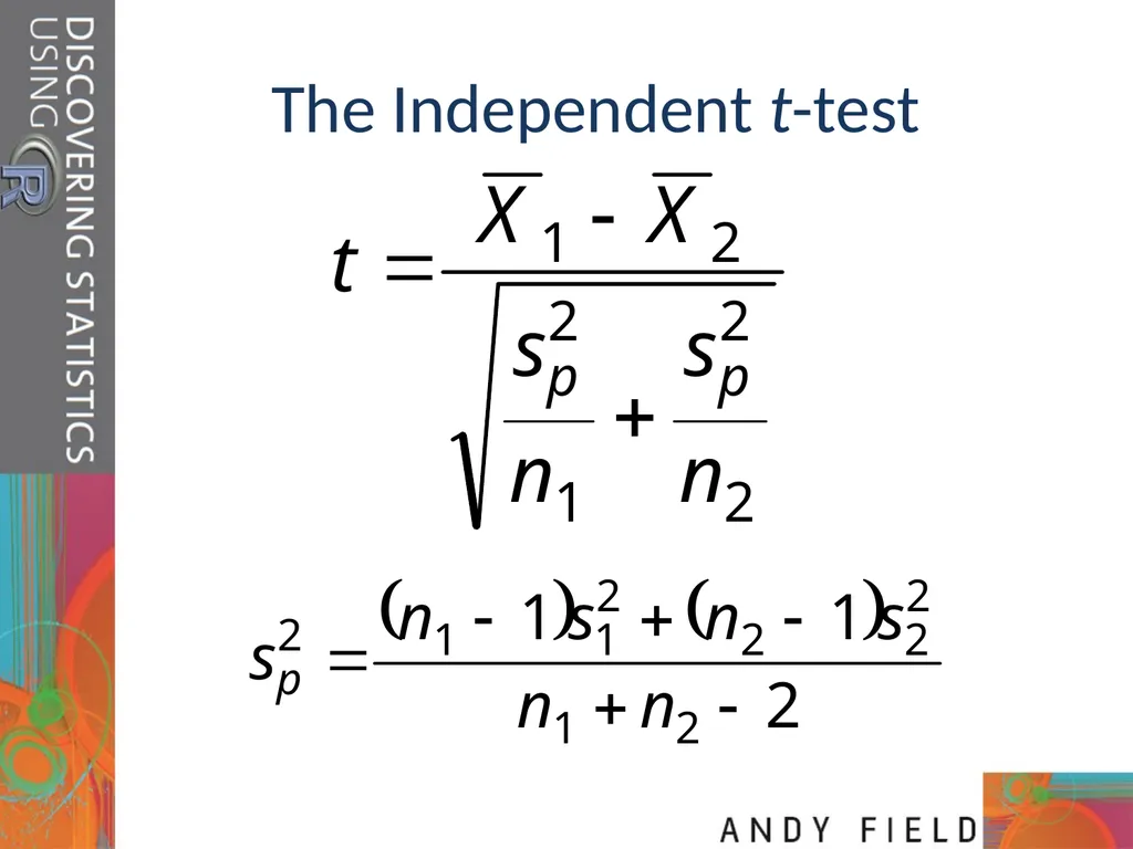
slide12. The Independent t-test<br>
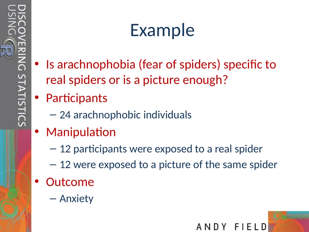
slide13. Example Is arachnophobia (fear of spiders) specific to real spiders or is a picture enough?
Participants
24 arachnophobic individuals
Manipulation
12 participants were exposed to a real spider
12 were exposed to a picture of the same spider
Outcome
Anxiety<br>
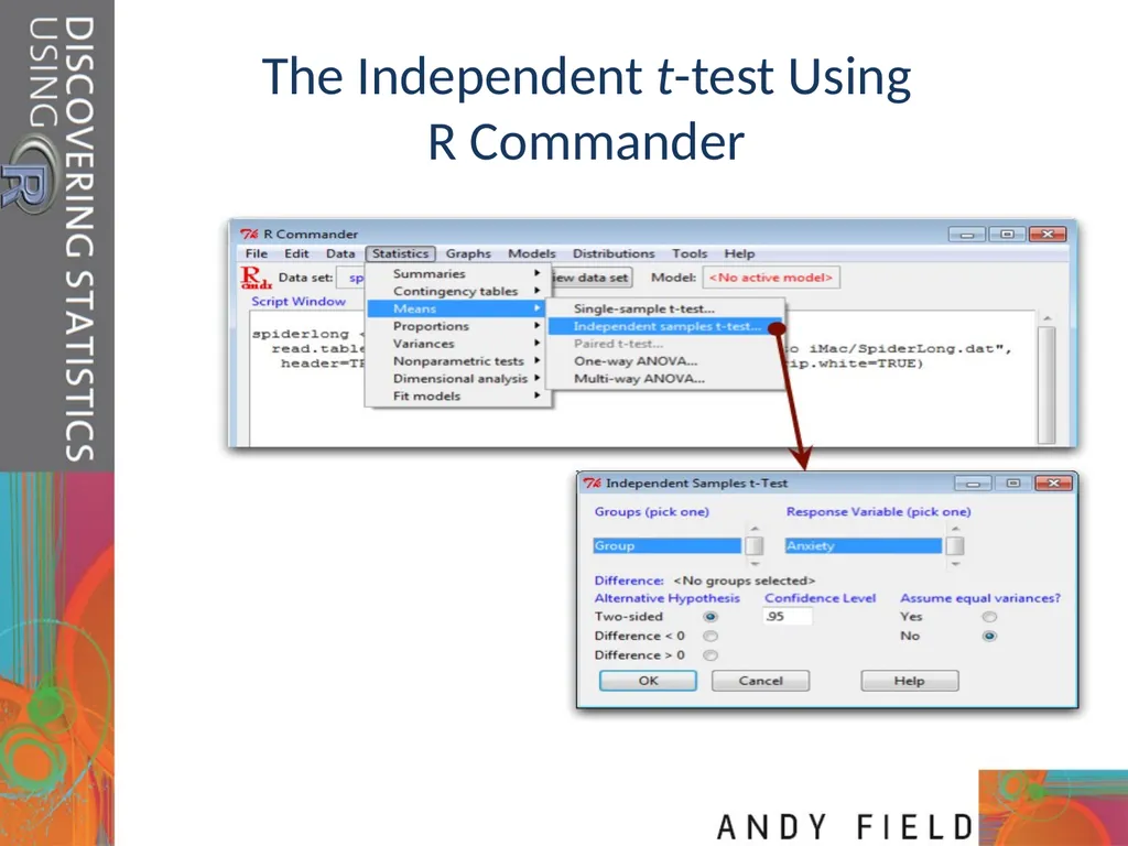
slide14. The Independent t-test Using R Commander<br>
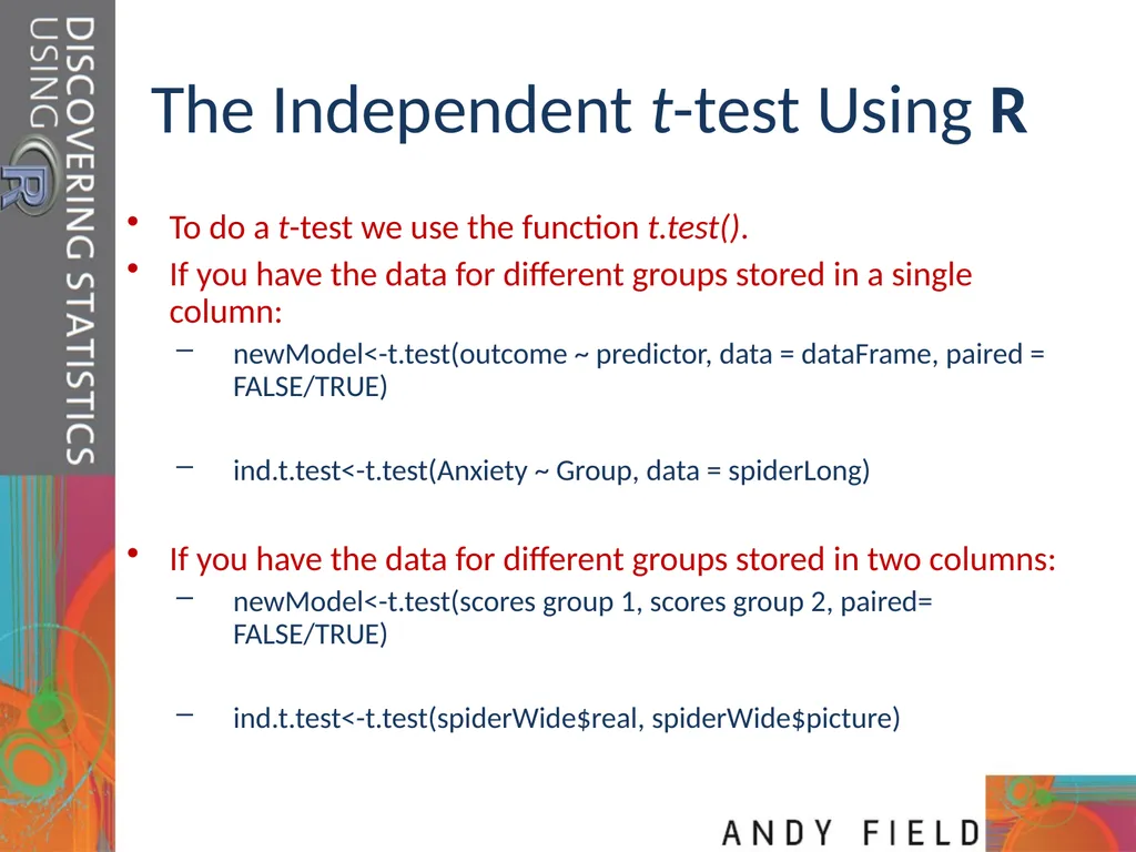
slide15. The Independent t-test Using R To do a t-test we use the function t.test().
If you have the data for different groups stored in a single column:
newModel<-t.test(outcome ~ predictor, data = dataFrame, paired = FALSE/TRUE)
ind.t.test<-t.test(Anxiety ~ Group, data = spiderLong)
If you have the data for different groups stored in two columns:
newModel<-t.test(scores group 1, scores group 2, paired= FALSE/TRUE)
ind.t.test<-t.test(spiderWide$real, spiderWide$picture)<br>
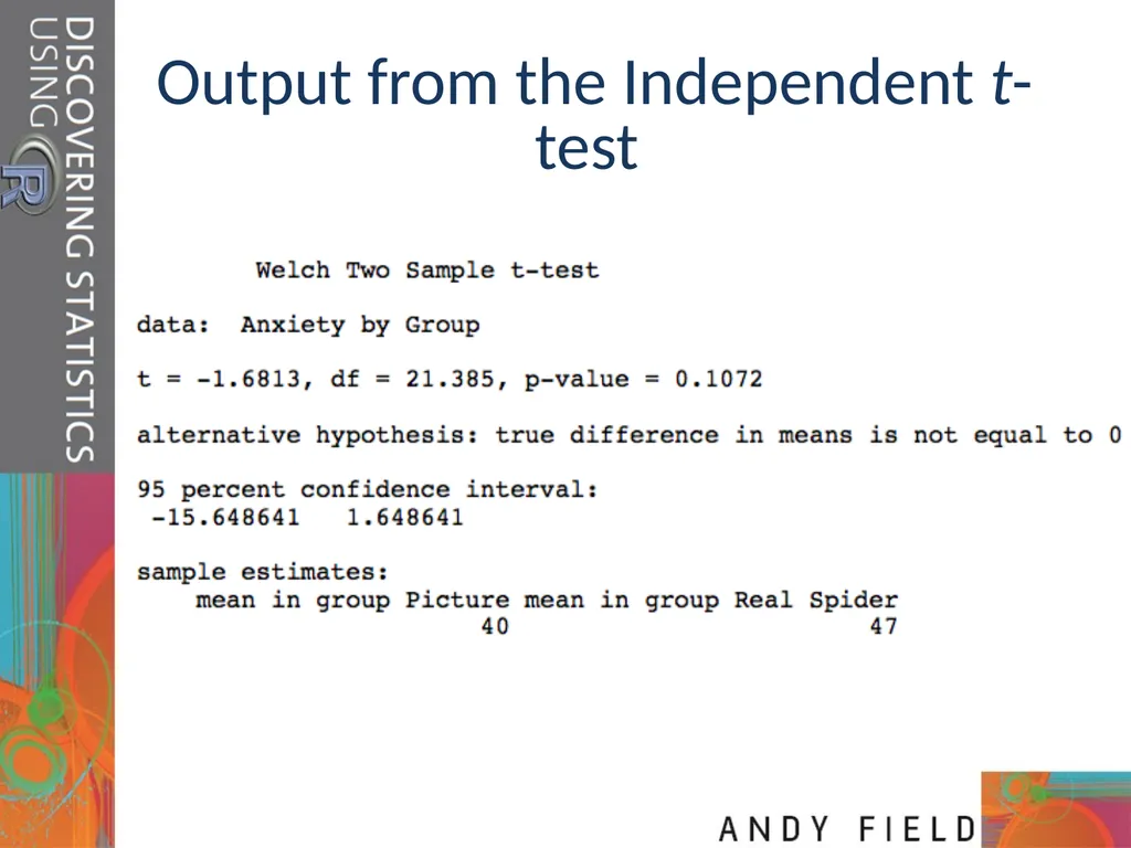
slide16. Output from the Independent t-test<br>
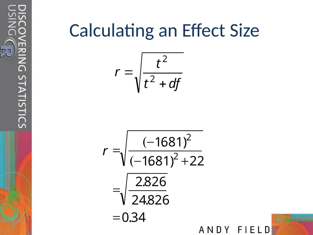
slide17. Calculating an Effect Size<br>
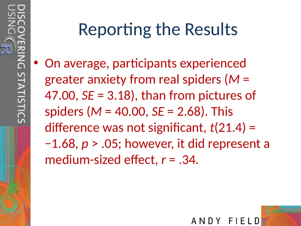
slide18. Reporting the Results On average, participants experienced greater anxiety from real spiders (M = 47.00, SE = 3.18), than from pictures of spiders (M = 40.00, SE = 2.68). This difference was not significant, t(21.4) = −1.68, p > .05; however, it did represent a medium-sized effect, r = .34.<br>
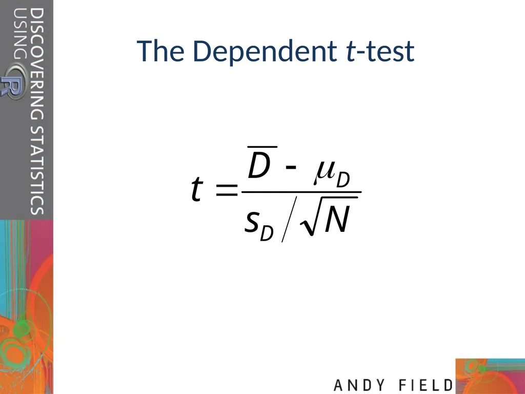
slide19. The Dependent t-test<br>
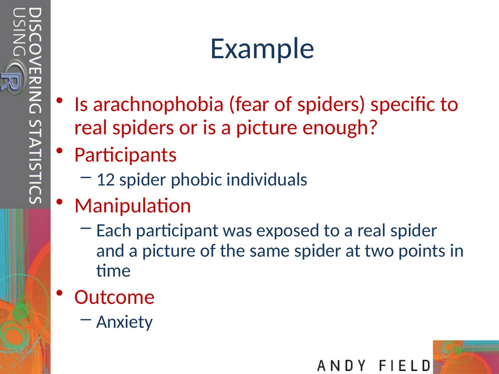
slide20. Example Is arachnophobia (fear of spiders) specific to real spiders or is a picture enough?
Participants
12 spider phobic individuals
Manipulation
Each participant was exposed to a real spider and a picture of the same spider at two points in time
Outcome
Anxiety<br>
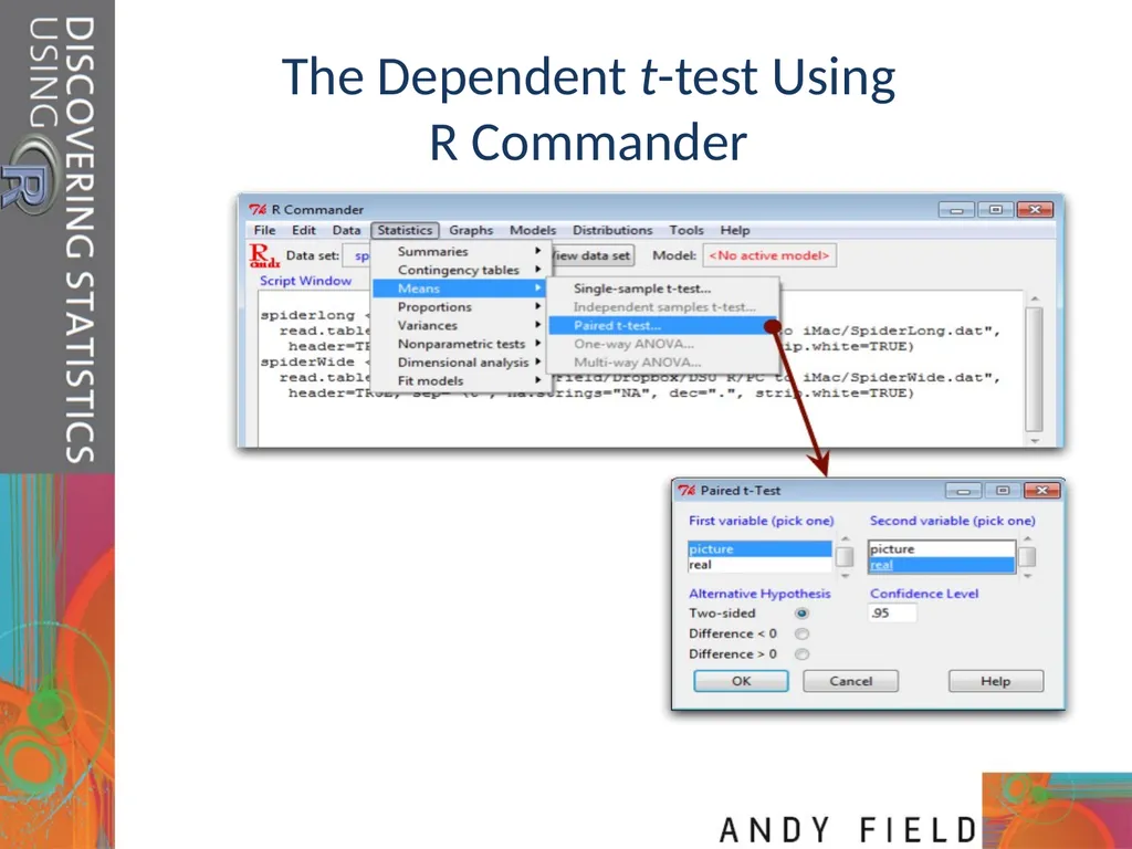
slide21. The Dependent t-test Using R Commander<br>
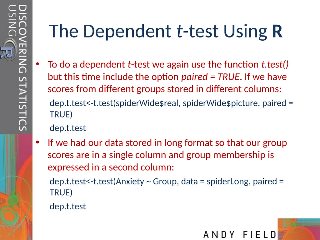
slide22. The Dependent t-test Using R To do a dependent t-test we again use the function t.test() but this time include the option paired = TRUE. If we have scores from different groups stored in different columns:
dep.t.test<-t.test(spiderWide$real, spiderWide$picture, paired = TRUE)
dep.t.test
If we had our data stored in long format so that our group scores are in a single column and group membership is expressed in a second column:
dep.t.test<-t.test(Anxiety ~ Group, data = spiderLong, paired = TRUE)
dep.t.test<br>
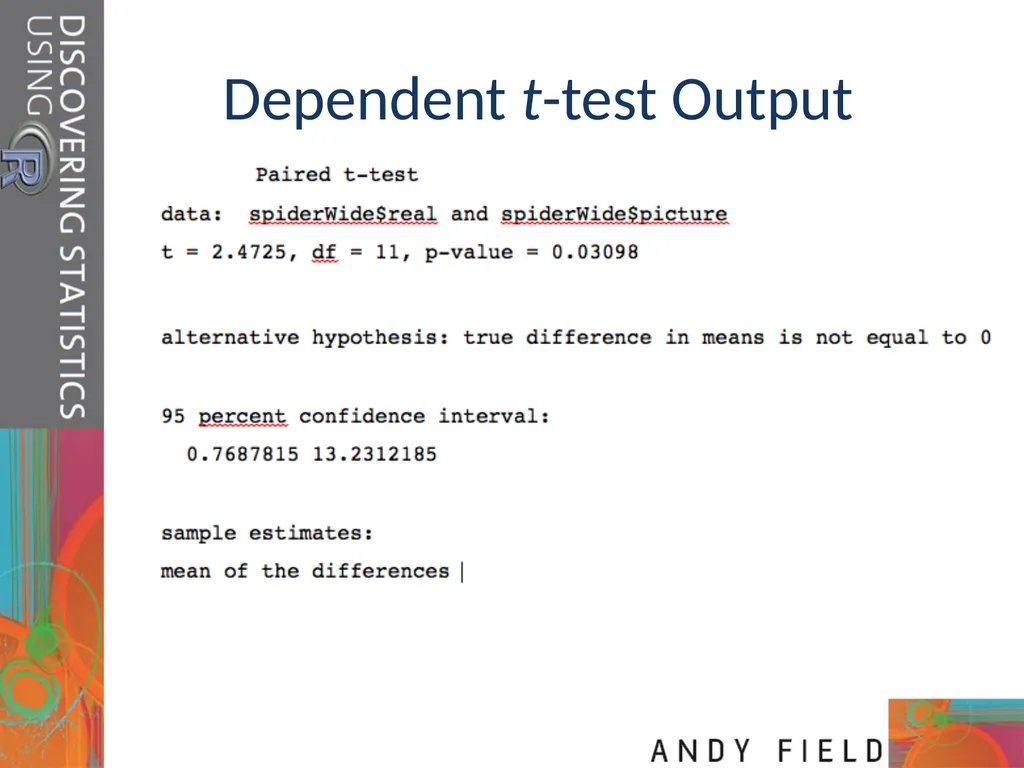
slide23. Dependent t-test Output<br>
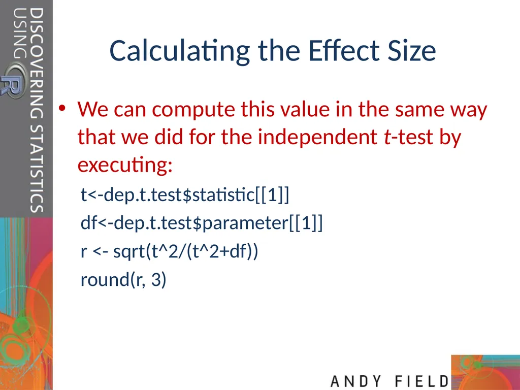
slide24. Calculating the Effect Size We can compute this value in the same way that we did for the independent t-test by executing:
t<-dep.t.test$statistic[[1]]
df<-dep.t.test$parameter[[1]]
r <- sqrt(t^2/(t^2+df))
round(r, 3)<br>
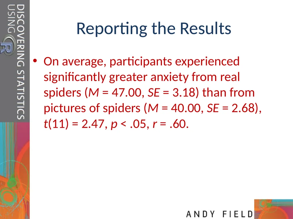
slide25. Reporting the Results On average, participants experienced significantly greater anxiety from real spiders (M = 47.00, SE = 3.18) than from pictures of spiders (M = 40.00, SE = 2.68), t(11) = 2.47, p < .05, r = .60.<br>
slide26. When Assumptions are Broken Dependent t-test
Mann–Whitney test
Wilcoxon rank-sum test
Independent t-test
Wilcoxon signed-rank test
Robust tests
Bootstrapping
Trimmed means<br>
slide27. Robust Methods to Compare Independent Means Regardless of whether your data come from the same or different entities, these functions require the data to be in two different columns (one for each experimental condition).<br>
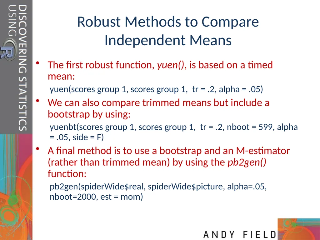
slide28. Robust Methods to Compare Independent Means The first robust function, yuen(), is based on a timed mean:
yuen(scores group 1, scores group 1, tr = .2, alpha = .05)
We can also compare trimmed means but include a bootstrap by using:
yuenbt(scores group 1, scores group 1, tr = .2, nboot = 599, alpha = .05, side = F)
A final method is to use a bootstrap and an M-estimator (rather than trimmed mean) by using the pb2gen() function:
pb2gen(spiderWide$real, spiderWide$picture, alpha=.05, nboot=2000, est = mom)<br>
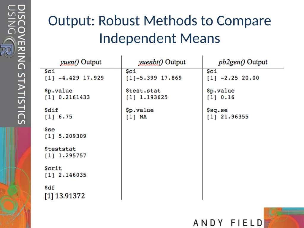
slide29. Output: Robust Methods to Compare Independent Means<br>
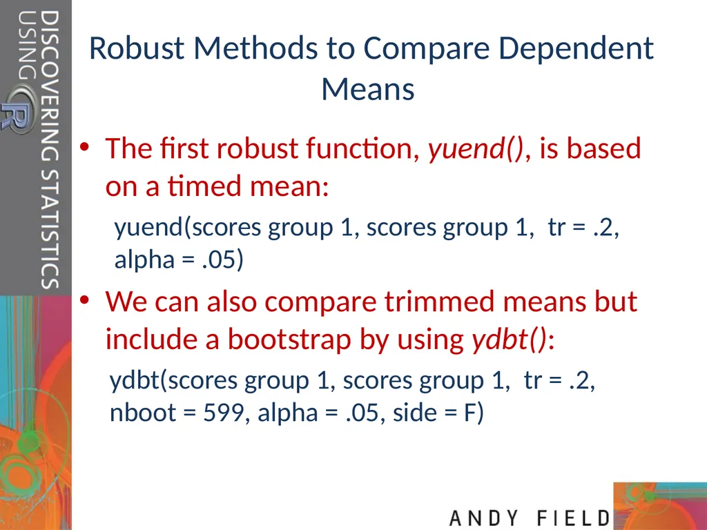
slide30. Robust Methods to Compare Dependent Means The first robust function, yuend(), is based on a timed mean:
yuend(scores group 1, scores group 1, tr = .2, alpha = .05)
We can also compare trimmed means but include a bootstrap by using ydbt():
ydbt(scores group 1, scores group 1, tr = .2, nboot = 599, alpha = .05, side = F)<br>
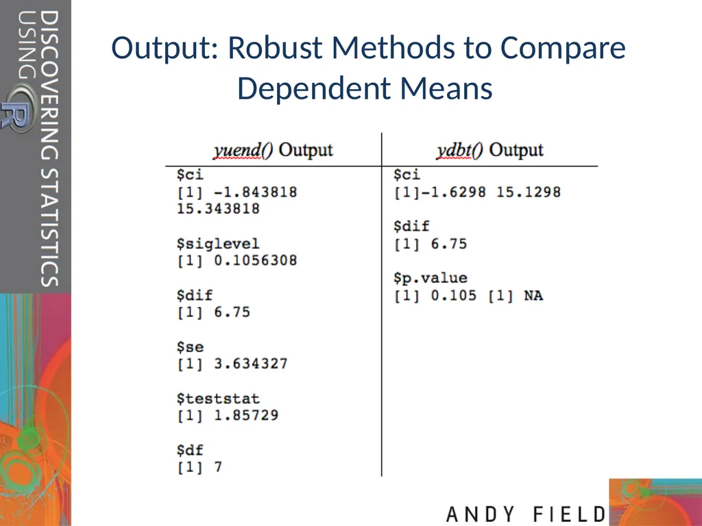
slide31. Output: Robust Methods to Compare Dependent Means<br>
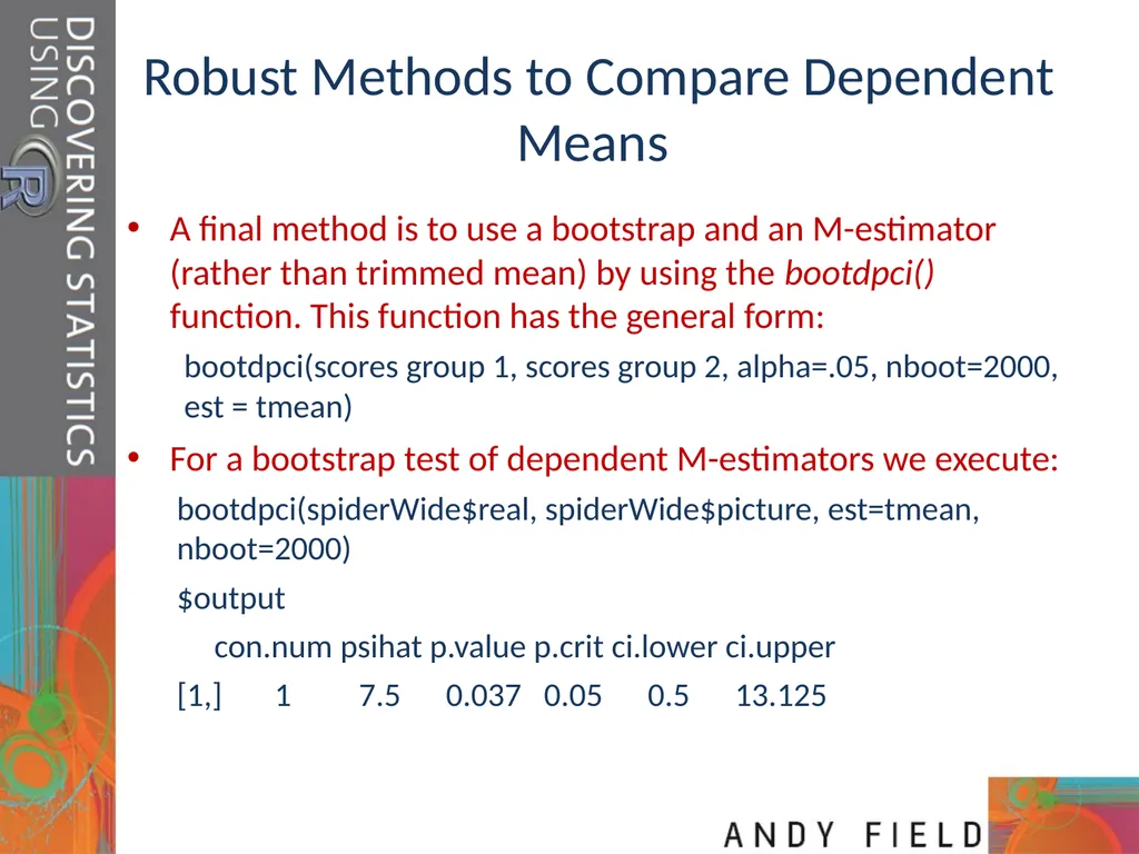
slide32. Robust Methods to Compare Dependent Means A final method is to use a bootstrap and an M-estimator (rather than trimmed mean) by using the bootdpci() function. This function has the general form:
bootdpci(scores group 1, scores group 2, alpha=.05, nboot=2000, est = tmean)
For a bootstrap test of dependent M-estimators we execute:
bootdpci(spiderWide$real, spiderWide$picture, est=tmean, nboot=2000)
$output
con.num psihat p.value p.crit ci.lower ci.upper
[1,] 1 7.5 0.037 0.05 0.5 13.125<br>
slide2. Aims t-tests:
Independent
Dependent (aka paired, matched)
Rationale for the tests
Assumptions
t-tests as a GLM
Interpretation
Calculating an effect size
Reporting results
Robust methods<br>
slide3. Experiments The simplest form of experiment that can be done is one with only one independent variable that is manipulated in only two ways and only one outcome is measured.
More often than not, the manipulation of the independent variable involves having an experimental condition and a control.
E.g., Is the movie Scream 2 scarier than the original Scream? We could measure heart rates (which indicate anxiety) during both films and compare them.
This situation can be analysed with a t-test<br>
slide4. t-test Independent t-test
Compares two means based on independent data.
E.g., data from different groups of people.
Dependent t-test
Compares two means based on related data.
E.g., Data from the same people measured at different times.
Data from ‘matched’ samples.
Significance testing
Testing the significance of Pearson’s correlation coefficient
Testing the significance of b in regression.<br>
slide5. Rationale for the t-test Two samples of data are collected and the sample means calculated. These means might differ by either a little or a lot.
If the samples come from the same population, then we expect their means to be roughly equal. Although it is possible for their means to differ by chance alone, we would expect large differences between sample means to occur very infrequently.
We compare the difference between the sample means that we collected to the difference between the sample means that we would expect to obtain if there were no effect (i.e. if the null hypothesis were true). We use the standard error as a gauge of the variability between sample means. If the difference between the samples we have collected is larger than what we would expect based on the standard error then we can assume one of two things:
There is no effect and sample means in our population fluctuate a lot and we have, by chance, collected two samples that are atypical of the population from which they came.
The two samples come from different populations but are typical of their respective parent population. In this scenario, the difference between samples represents a genuine difference between the samples (and so the null hypothesis is incorrect).
As the observed difference between the sample means gets larger, the more confident we become that the second explanation is correct (i.e. that the null hypothesis should be rejected). If the null hypothesis is incorrect, then we gain confidence that the two sample means differ because of the different experimental manipulation imposed on each sample.<br>
slide6. Rationale for the t-test<br>
slide7. The t-test as a GLM<br>
slide8. Picture Group The group variable = 0
Intercept = mean of baseline group<br>
slide9. Real Spider Group The group variable = 1
b1 = Difference between means<br>
slide10. Output from a Regression<br>
slide11. Assumptions of the t-test Both the independent t-test and the dependent t-test are parametric tests based on the normal distribution. Therefore, they assume:
The sampling distribution is normally distributed. In the dependent ttest this means that the sampling distribution of the differences between scores should be normal, not the scores themselves.
Data are measured at least at the interval level.
The independent t-test, because it is used to test different groups of people, also assumes:
Variances in these populations are roughly equal (homogeneity of variance).
Scores in different treatment conditions are independent (because they come from different people).<br>
slide12. The Independent t-test<br>
slide13. Example Is arachnophobia (fear of spiders) specific to real spiders or is a picture enough?
Participants
24 arachnophobic individuals
Manipulation
12 participants were exposed to a real spider
12 were exposed to a picture of the same spider
Outcome
Anxiety<br>
slide14. The Independent t-test Using R Commander<br>
slide15. The Independent t-test Using R To do a t-test we use the function t.test().
If you have the data for different groups stored in a single column:
newModel<-t.test(outcome ~ predictor, data = dataFrame, paired = FALSE/TRUE)
ind.t.test<-t.test(Anxiety ~ Group, data = spiderLong)
If you have the data for different groups stored in two columns:
newModel<-t.test(scores group 1, scores group 2, paired= FALSE/TRUE)
ind.t.test<-t.test(spiderWide$real, spiderWide$picture)<br>
slide16. Output from the Independent t-test<br>
slide17. Calculating an Effect Size<br>
slide18. Reporting the Results On average, participants experienced greater anxiety from real spiders (M = 47.00, SE = 3.18), than from pictures of spiders (M = 40.00, SE = 2.68). This difference was not significant, t(21.4) = −1.68, p > .05; however, it did represent a medium-sized effect, r = .34.<br>
slide19. The Dependent t-test<br>
slide20. Example Is arachnophobia (fear of spiders) specific to real spiders or is a picture enough?
Participants
12 spider phobic individuals
Manipulation
Each participant was exposed to a real spider and a picture of the same spider at two points in time
Outcome
Anxiety<br>
slide21. The Dependent t-test Using R Commander<br>
slide22. The Dependent t-test Using R To do a dependent t-test we again use the function t.test() but this time include the option paired = TRUE. If we have scores from different groups stored in different columns:
dep.t.test<-t.test(spiderWide$real, spiderWide$picture, paired = TRUE)
dep.t.test
If we had our data stored in long format so that our group scores are in a single column and group membership is expressed in a second column:
dep.t.test<-t.test(Anxiety ~ Group, data = spiderLong, paired = TRUE)
dep.t.test<br>
slide23. Dependent t-test Output<br>
slide24. Calculating the Effect Size We can compute this value in the same way that we did for the independent t-test by executing:
t<-dep.t.test$statistic[[1]]
df<-dep.t.test$parameter[[1]]
r <- sqrt(t^2/(t^2+df))
round(r, 3)<br>
slide25. Reporting the Results On average, participants experienced significantly greater anxiety from real spiders (M = 47.00, SE = 3.18) than from pictures of spiders (M = 40.00, SE = 2.68), t(11) = 2.47, p < .05, r = .60.<br>
slide26. When Assumptions are Broken Dependent t-test
Mann–Whitney test
Wilcoxon rank-sum test
Independent t-test
Wilcoxon signed-rank test
Robust tests
Bootstrapping
Trimmed means<br>
slide27. Robust Methods to Compare Independent Means Regardless of whether your data come from the same or different entities, these functions require the data to be in two different columns (one for each experimental condition).<br>
slide28. Robust Methods to Compare Independent Means The first robust function, yuen(), is based on a timed mean:
yuen(scores group 1, scores group 1, tr = .2, alpha = .05)
We can also compare trimmed means but include a bootstrap by using:
yuenbt(scores group 1, scores group 1, tr = .2, nboot = 599, alpha = .05, side = F)
A final method is to use a bootstrap and an M-estimator (rather than trimmed mean) by using the pb2gen() function:
pb2gen(spiderWide$real, spiderWide$picture, alpha=.05, nboot=2000, est = mom)<br>
slide29. Output: Robust Methods to Compare Independent Means<br>
slide30. Robust Methods to Compare Dependent Means The first robust function, yuend(), is based on a timed mean:
yuend(scores group 1, scores group 1, tr = .2, alpha = .05)
We can also compare trimmed means but include a bootstrap by using ydbt():
ydbt(scores group 1, scores group 1, tr = .2, nboot = 599, alpha = .05, side = F)<br>
slide31. Output: Robust Methods to Compare Dependent Means<br>
slide32. Robust Methods to Compare Dependent Means A final method is to use a bootstrap and an M-estimator (rather than trimmed mean) by using the bootdpci() function. This function has the general form:
bootdpci(scores group 1, scores group 2, alpha=.05, nboot=2000, est = tmean)
For a bootstrap test of dependent M-estimators we execute:
bootdpci(spiderWide$real, spiderWide$picture, est=tmean, nboot=2000)
$output
con.num psihat p.value p.crit ci.lower ci.upper
[1,] 1 7.5 0.037 0.05 0.5 13.125<br>