
Compressible Flow Analysis for High-Speed Vehicles





Description: Compressible Flow Analysis for High-Speed Vehicles Vincent Cuda, Jr., Ph.D., P.E. AMANASA LaRC Important Questions Integrated Approach For Hypersonic Vehicle Designs What constitutes a complete research effort? How do various Systems
Related Topics
Download Presentation
"Compressible Flow Analysis for High-Speed Vehicles" is the property of its rightful owner. Permission is granted to download and print the materials on this website for personal, non-commercial use only, and to display it on your personal computer provided you do not modify the materials and that you retain all copyright notices contained in the materials. By downloading content from our website, you accept the terms of this agreement.
Presentation Transcript
slide1. Compressible Flow Analysis for High-Speed Vehicles Vincent Cuda, Jr., Ph.D., P.E.
AMA/NASA LaRC<br>
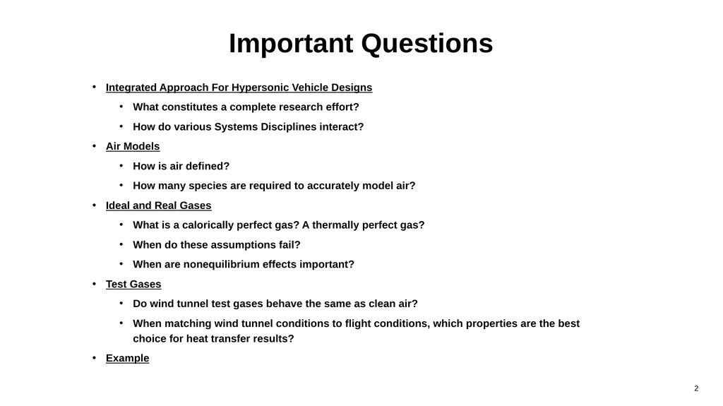
slide2. Important Questions Integrated Approach For Hypersonic Vehicle Designs
What constitutes a complete research effort?
How do various Systems Disciplines interact?
Air Models
How is air defined?
How many species are required to accurately model air?
Ideal and Real Gases
What is a calorically perfect gas? A thermally perfect gas?
When do these assumptions fail?
When are nonequilibrium effects important?
Test Gases
Do wind tunnel test gases behave the same as clean air?
When matching wind tunnel conditions to flight conditions, which properties are the best choice for heat transfer results?
Example<br>
slide3. Hypersonic Scramjet Flowpath Development Flight Test Ground Test Simulation Verification of flight bridging
Data for analytical model development Design database and trade studies. Test interpretation and analysis of off-trajectory points Quantification of facility/model effects Facility/model configuration assessment and gauge placement. Data consistency and test interpretation Verification of computational methodology.
Data for analytical model development. Design database and parametric testing
Viable scramjet operation that meets objectives<br>
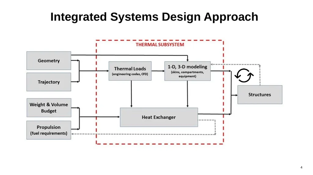
slide4. Integrated Systems Design Approach<br>
slide5. Air<br>
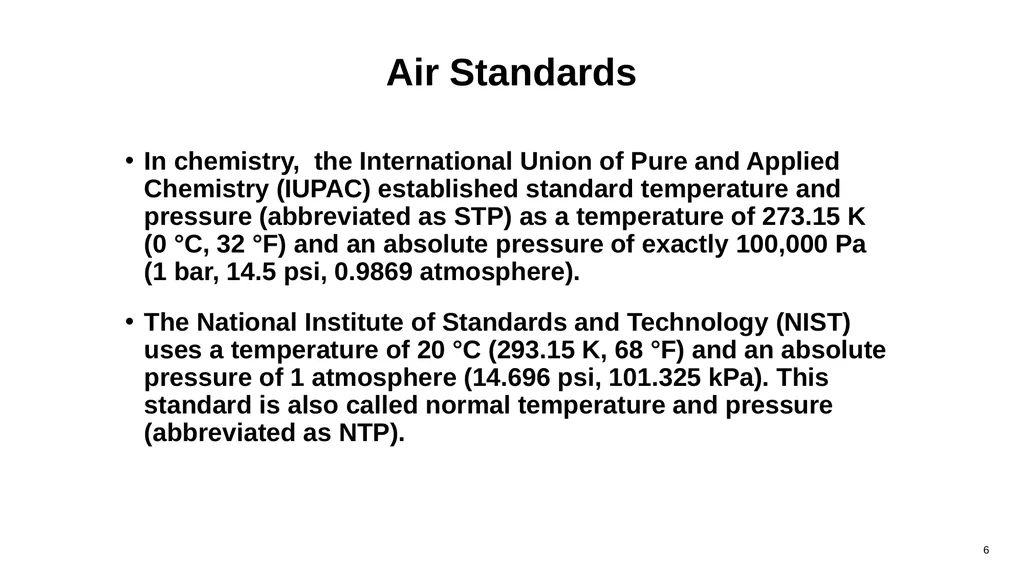
slide6. Air Standards In chemistry, the International Union of Pure and Applied Chemistry (IUPAC) established standard temperature and pressure (abbreviated as STP) as a temperature of 273.15 K (0 °C, 32 °F) and an absolute pressure of exactly 100,000 Pa (1 bar, 14.5 psi, 0.9869 atmosphere).
The National Institute of Standards and Technology (NIST) uses a temperature of 20 °C (293.15 K, 68 °F) and an absolute pressure of 1 atmosphere (14.696 psi, 101.325 kPa). This standard is also called normal temperature and pressure (abbreviated as NTP).<br>
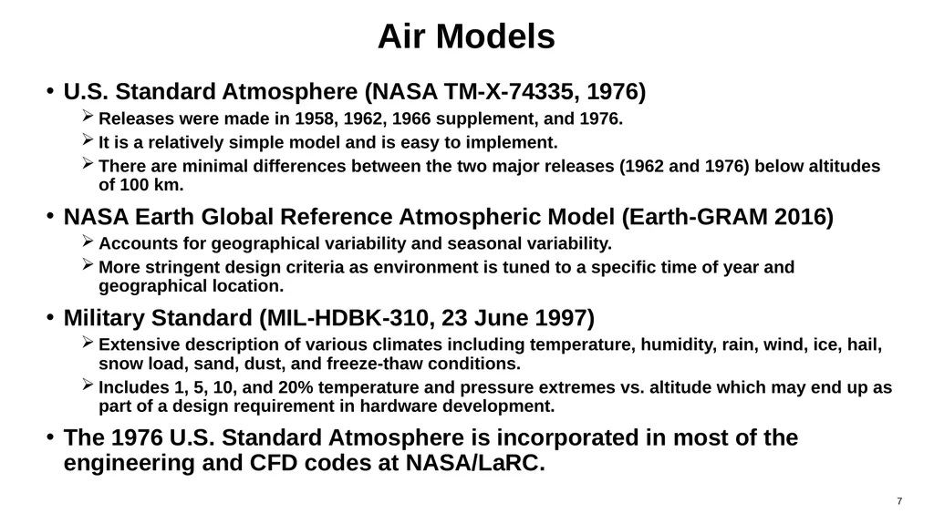
slide7. Air Models U.S. Standard Atmosphere (NASA TM-X-74335, 1976)
Releases were made in 1958, 1962, 1966 supplement, and 1976.
It is a relatively simple model and is easy to implement.
There are minimal differences between the two major releases (1962 and 1976) below altitudes of 100 km.
NASA Earth Global Reference Atmospheric Model (Earth-GRAM 2016)
Accounts for geographical variability and seasonal variability.
More stringent design criteria as environment is tuned to a specific time of year and geographical location.
Military Standard (MIL-HDBK-310, 23 June 1997)
Extensive description of various climates including temperature, humidity, rain, wind, ice, hail, snow load, sand, dust, and freeze-thaw conditions.
Includes 1, 5, 10, and 20% temperature and pressure extremes vs. altitude which may end up as part of a design requirement in hardware development.
The 1976 U.S. Standard Atmosphere is incorporated in most of the engineering and CFD codes at NASA/LaRC.<br>
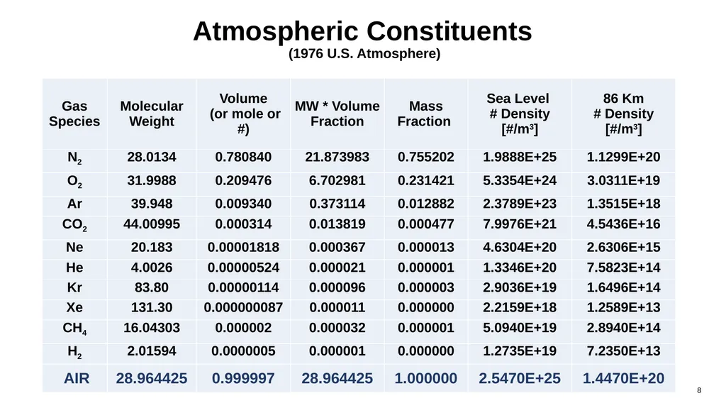
slide8. Atmospheric Constituents (1976 U.S. Atmosphere)<br>
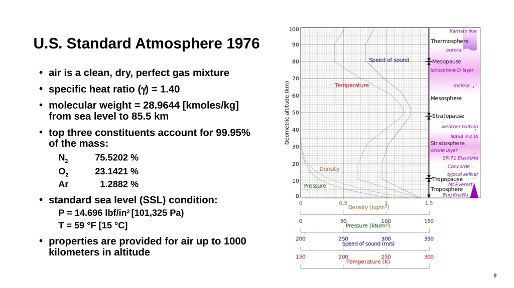
slide9. U.S. Standard Atmosphere 1976 air is a clean, dry, perfect gas mixture
specific heat ratio (g) = 1.40
molecular weight = 28.9644 [kmoles/kg] from sea level to 85.5 km
top three constituents account for 99.95% of the mass:
N2 75.5202 %
O2 23.1421 %
Ar 1.2882 %
standard sea level (SSL) condition:
P = 14.696 lbf/in2 [101,325 Pa)
T = 59 °F [15 °C]
properties are provided for air up to 1000 kilometers in altitude<br>
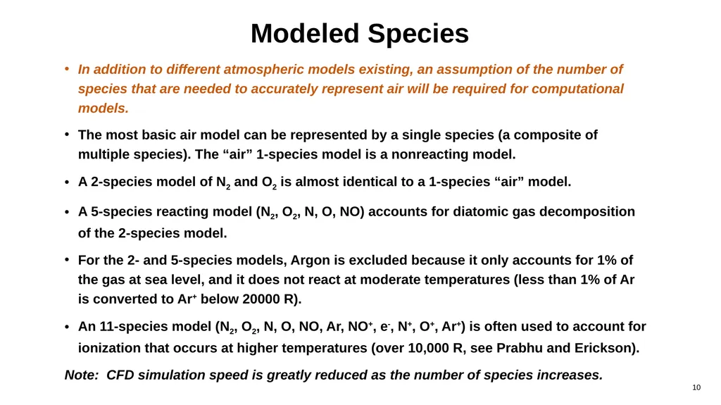
slide10. Modeled Species In addition to different atmospheric models existing, an assumption of the number of species that are needed to accurately represent air will be required for computational models.
The most basic air model can be represented by a single species (a composite of multiple species). The “air” 1-species model is a nonreacting model.
A 2-species model of N2 and O2 is almost identical to a 1-species “air” model.
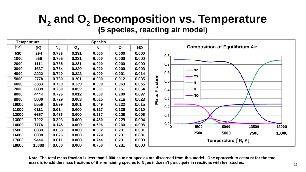
A 5-species reacting model (N2, O2, N, O, NO) accounts for diatomic gas decomposition of the 2-species model.
For the 2- and 5-species models, Argon is excluded because it only accounts for 1% of the gas at sea level, and it does not react at moderate temperatures (less than 1% of Ar is converted to Ar+ below 20000 R).
An 11-species model (N2, O2, N, O, NO, Ar, NO+, e-, N+, O+, Ar+) is often used to account for ionization that occurs at higher temperatures (over 10,000 R, see Prabhu and Erickson).
Note: CFD simulation speed is greatly reduced as the number of species increases.<br>
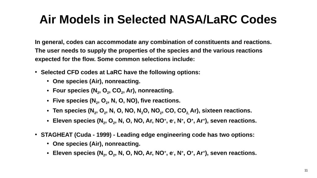
slide11. Air Models in Selected NASA/LaRC Codes In general, codes can accommodate any combination of constituents and reactions. The user needs to supply the properties of the species and the various reactions expected for the flow. Some common selections include:
Selected CFD codes at LaRC have the following options:
One species (Air), nonreacting.
Four species (N2, O2, CO2, Ar), nonreacting.
Five species (N2, O2, N, O, NO), five reactions.
Ten species (N2, O2, N, O, NO, N2O, NO2, CO, CO2, Ar), sixteen reactions.
Eleven species (N2, O2, N, O, NO, Ar, NO+, e-, N+, O+, Ar+), seven reactions.
STAGHEAT (Cuda - 1999) - Leading edge engineering code has two options:
One species (Air), nonreacting.
Eleven species (N2, O2, N, O, NO, Ar, NO+, e-, N+, O+, Ar+), seven reactions.<br>
slide12. N2 and O2 Decomposition vs. Temperature (5 species, reacting air model) Note: The total mass fraction is less than 1.000 as minor species are discarded from this model. One approach to account for the total mass is to add the mass fractions of the remaining species to N2 as it doesn’t participate in reactions with fuel studies.<br>
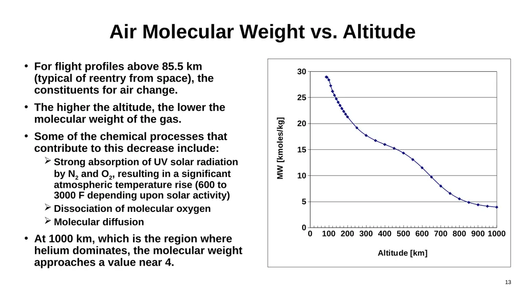
slide13. Air Molecular Weight vs. Altitude For flight profiles above 85.5 km (typical of reentry from space), the constituents for air change.
The higher the altitude, the lower the molecular weight of the gas.
Some of the chemical processes that contribute to this decrease include:
Strong absorption of UV solar radiation by N2 and O2, resulting in a significant atmospheric temperature rise (600 to 3000 F depending upon solar activity)
Dissociation of molecular oxygen
Molecular diffusion
At 1000 km, which is the region where helium dominates, the molecular weight approaches a value near 4.<br>
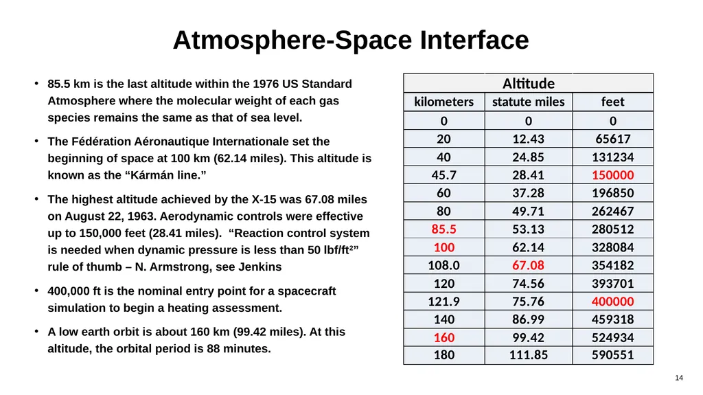
slide14. Atmosphere-Space Interface 85.5 km is the last altitude within the 1976 US Standard Atmosphere where the molecular weight of each gas species remains the same as that of sea level.
The Fédération Aéronautique Internationale set the beginning of space at 100 km (62.14 miles). This altitude is known as the “Kármán line.”
The highest altitude achieved by the X-15 was 67.08 miles on August 22, 1963. Aerodynamic controls were effective up to 150,000 feet (28.41 miles). “Reaction control system is needed when dynamic pressure is less than 50 lbf/ft2” rule of thumb – N. Armstrong, see Jenkins
400,000 ft is the nominal entry point for a spacecraft simulation to begin a heating assessment.
A low earth orbit is about 160 km (99.42 miles). At this altitude, the orbital period is 88 minutes.<br>
slide15. Real Gases and Compressible Flows<br>
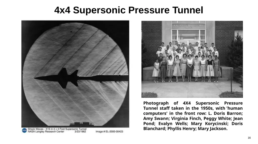
slide16. Photograph of 4X4 Supersonic Pressure Tunnel staff taken in the 1950s, with 'human computers' in the front row: L. Doris Barron; Amy Swann; Virginia Finch, Peggy White; Jean Pond; Evalyn Wells; Mary Korycinski; Doris Blanchard; Phyllis Henry; Mary Jackson. 4x4 Supersonic Pressure Tunnel<br>
slide17. How was the Ideal Gas Law was Discovered? Based on four variables, there are six different possible trends that can be established for two properties while holding the other two constant (varying two of P, V, T, n while holding the other two constant; note that the gas constant, R, does not vary). Four of these six trends were named. After the named trends were discovered, the comprehensive ideal gas law expression was developed which satisfies each of the original studies.
P – Absolute Pressure [Pa]
V – Volume [m3]
T – Absolute Temperature [K]
n – number of moles [moles]
R – Gas Constant 8.314 [J/moles-K]<br>
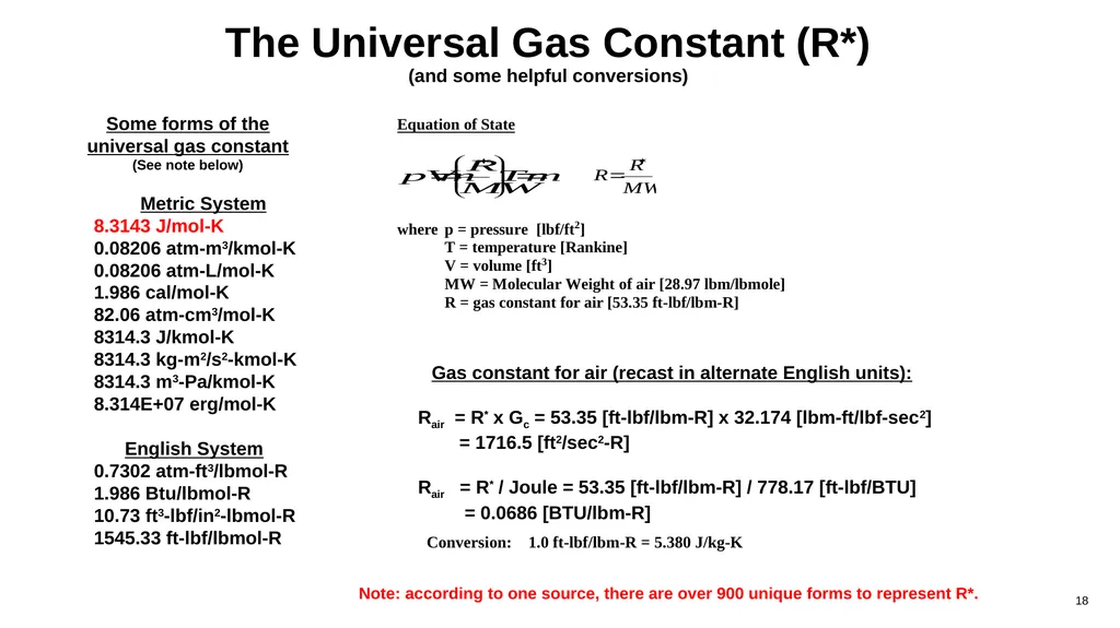
slide18. The Universal Gas Constant (R*) (and some helpful conversions) Metric System
8.3143 J/mol-K
0.08206 atm-m3/kmol-K
0.08206 atm-L/mol-K
1.986 cal/mol-K
82.06 atm-cm3/mol-K
8314.3 J/kmol-K
8314.3 kg-m2/s2-kmol-K
8314.3 m3-Pa/kmol-K
8.314E+07 erg/mol-K
English System
0.7302 atm-ft3/lbmol-R
1.986 Btu/lbmol-R
10.73 ft3-lbf/in2-lbmol-R
1545.33 ft-lbf/lbmol-R Gas constant for air (recast in alternate English units):
Rair = R* x Gc = 53.35 [ft-lbf/lbm-R] x 32.174 [lbm-ft/lbf-sec2]
= 1716.5 [ft2/sec2-R]
Rair = R* / Joule = 53.35 [ft-lbf/lbm-R] / 778.17 [ft-lbf/BTU]
= 0.0686 [BTU/lbm-R] Note: according to one source, there are over 900 unique forms to represent R*. Some forms of the universal gas constant (See note below)<br>
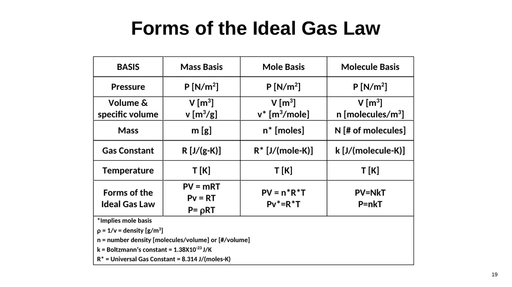
slide19. Forms of the Ideal Gas Law<br>
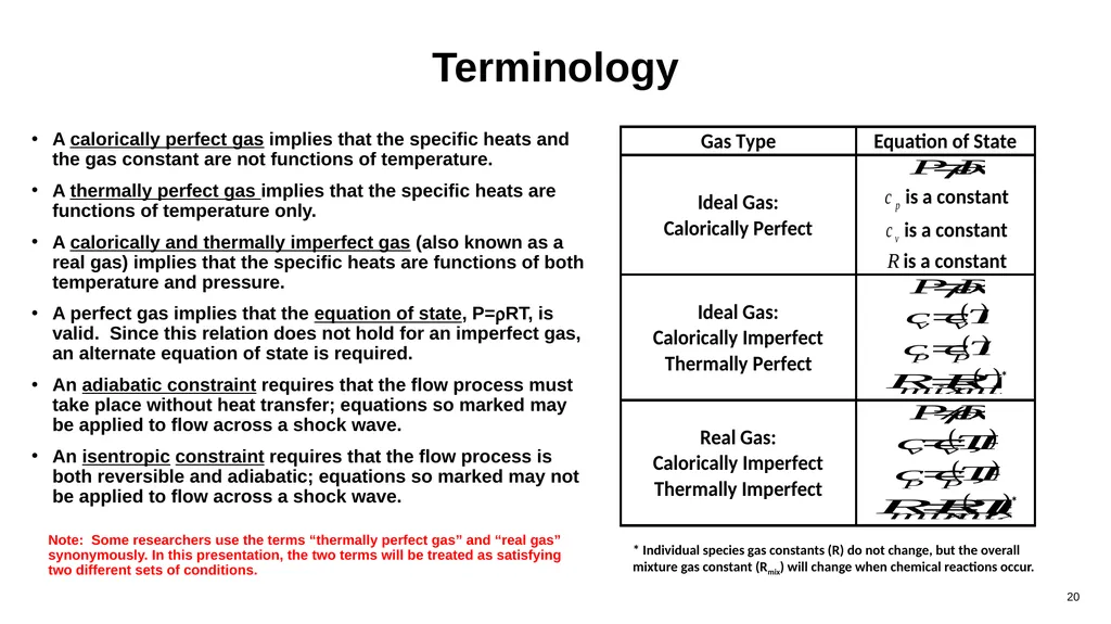
slide20. Terminology A calorically perfect gas implies that the specific heats and the gas constant are not functions of temperature.
A thermally perfect gas implies that the specific heats are functions of temperature only.
A calorically and thermally imperfect gas (also known as a real gas) implies that the specific heats are functions of both temperature and pressure.
A perfect gas implies that the equation of state, P=rRT, is valid. Since this relation does not hold for an imperfect gas, an alternate equation of state is required.
An adiabatic constraint requires that the flow process must take place without heat transfer; equations so marked may be applied to flow across a shock wave.
An isentropic constraint requires that the flow process is both reversible and adiabatic; equations so marked may not be applied to flow across a shock wave.
Note: Some researchers use the terms “thermally perfect gas” and “real gas” synonymously. In this presentation, the two terms will be treated as satisfying two different sets of conditions. * Individual species gas constants (R) do not change, but the overall mixture gas constant (Rmix) will change when chemical reactions occur.<br>
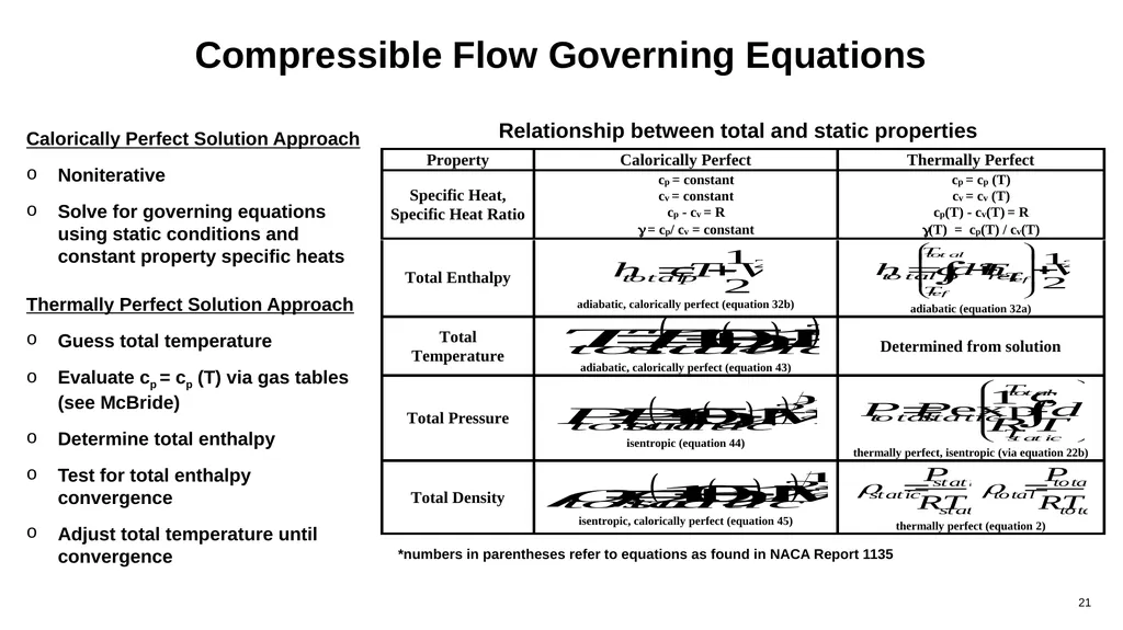
slide21. Compressible Flow Governing Equations Thermally Perfect Solution Approach
Guess total temperature
Evaluate cp = cp (T) via gas tables (see McBride)
Determine total enthalpy
Test for total enthalpy convergence
Adjust total temperature until convergence Calorically Perfect Solution Approach
Noniterative
Solve for governing equations using static conditions and constant property specific heats Relationship between total and static properties *numbers in parentheses refer to equations as found in NACA Report 1135<br>
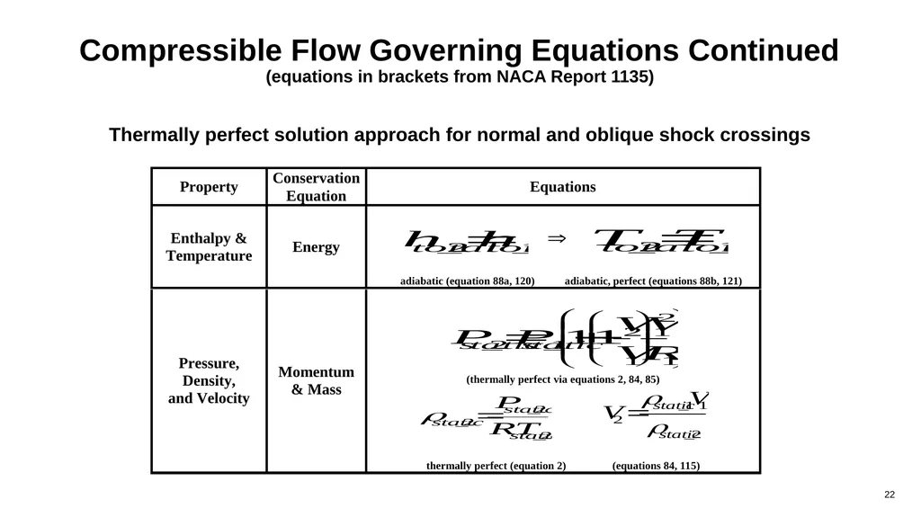
slide22. Compressible Flow Governing Equations Continued (equations in brackets from NACA Report 1135) Thermally perfect solution approach for normal and oblique shock crossings<br>
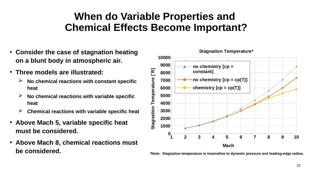
slide23. When do Variable Properties and Chemical Effects Become Important? Consider the case of stagnation heating on a blunt body in atmospheric air.
Three models are illustrated:
No chemical reactions with constant specific heat
No chemical reactions with variable specific heat
Chemical reactions with variable specific heat
Above Mach 5, variable specific heat must be considered.
Above Mach 8, chemical reactions must be considered. *Note: Stagnation temperature is insensitive to dynamic pressure and leading-edge radius.<br>
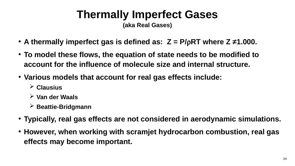
slide24. Thermally Imperfect Gases (aka Real Gases) A thermally imperfect gas is defined as: Z = P/rRT where Z ≠1.000.
To model these flows, the equation of state needs to be modified to account for the influence of molecule size and internal structure.
Various models that account for real gas effects include:
Clausius
Van der Waals
Beattie-Bridgmann
Typically, real gas effects are not considered in aerodynamic simulations.
However, when working with scramjet hydrocarbon combustion, real gas effects may become important.<br>
slide25. Additional Considerations Nonequilibrium Flows
Thermally Imperfect Gases
Regions Requiring Special Attention<br>
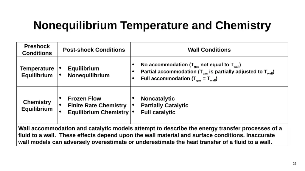
slide26. Nonequilibrium Temperature and Chemistry<br>
slide27. Ground Test Gases<br>
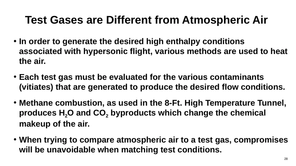
slide28. Test Gases are Different from Atmospheric Air In order to generate the desired high enthalpy conditions associated with hypersonic flight, various methods are used to heat the air.
Each test gas must be evaluated for the various contaminants (vitiates) that are generated to produce the desired flow conditions.
Methane combustion, as used in the 8-Ft. High Temperature Tunnel, produces H2O and CO2 byproducts which change the chemical makeup of the air.
When trying to compare atmospheric air to a test gas, compromises will be unavoidable when matching test conditions.<br>
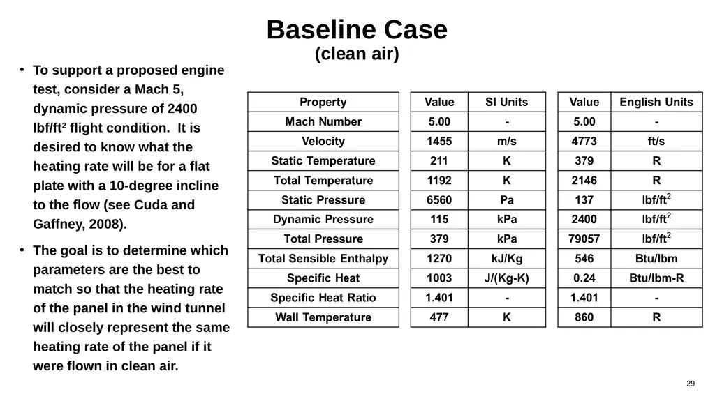
slide29. Baseline Case (clean air) To support a proposed engine test, consider a Mach 5, dynamic pressure of 2400 lbf/ft2 flight condition. It is desired to know what the heating rate will be for a flat plate with a 10-degree incline to the flow (see Cuda and Gaffney, 2008).
The goal is to determine which parameters are the best to match so that the heating rate of the panel in the wind tunnel will closely represent the same heating rate of the panel if it were flown in clean air.<br>
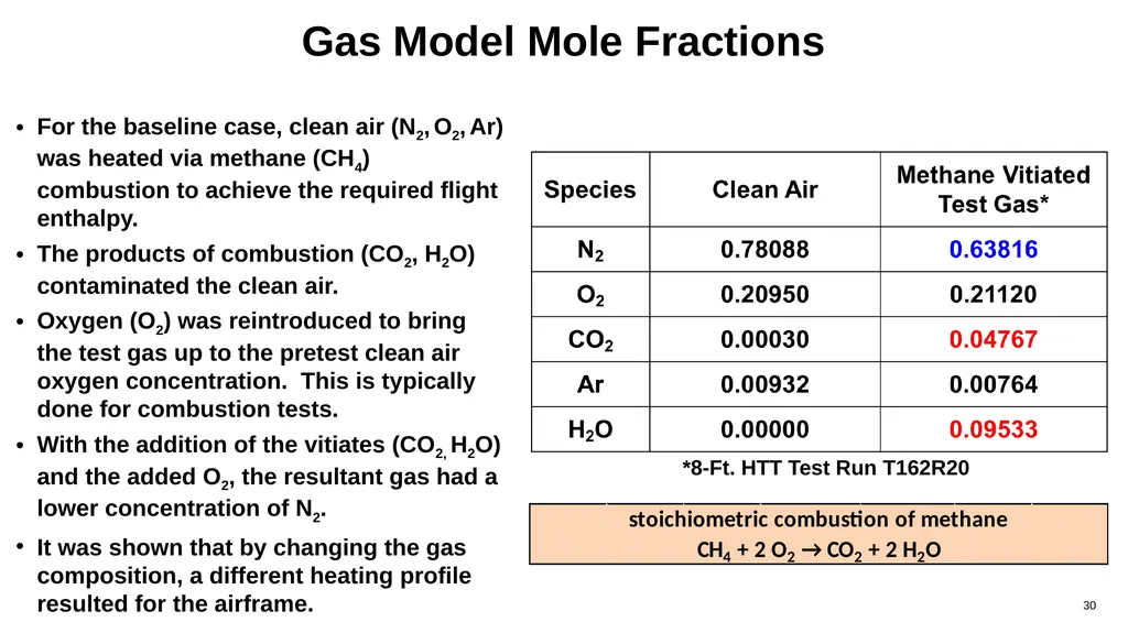
slide30. Gas Model Mole Fractions For the baseline case, clean air (N2, O2, Ar) was heated via methane (CH4) combustion to achieve the required flight enthalpy.
The products of combustion (CO2, H2O) contaminated the clean air.
Oxygen (O2) was reintroduced to bring the test gas up to the pretest clean air oxygen concentration. This is typically done for combustion tests.
With the addition of the vitiates (CO2, H2O) and the added O2, the resultant gas had a lower concentration of N2.
It was shown that by changing the gas composition, a different heating profile resulted for the airframe. *8-Ft. HTT Test Run T162R20<br>
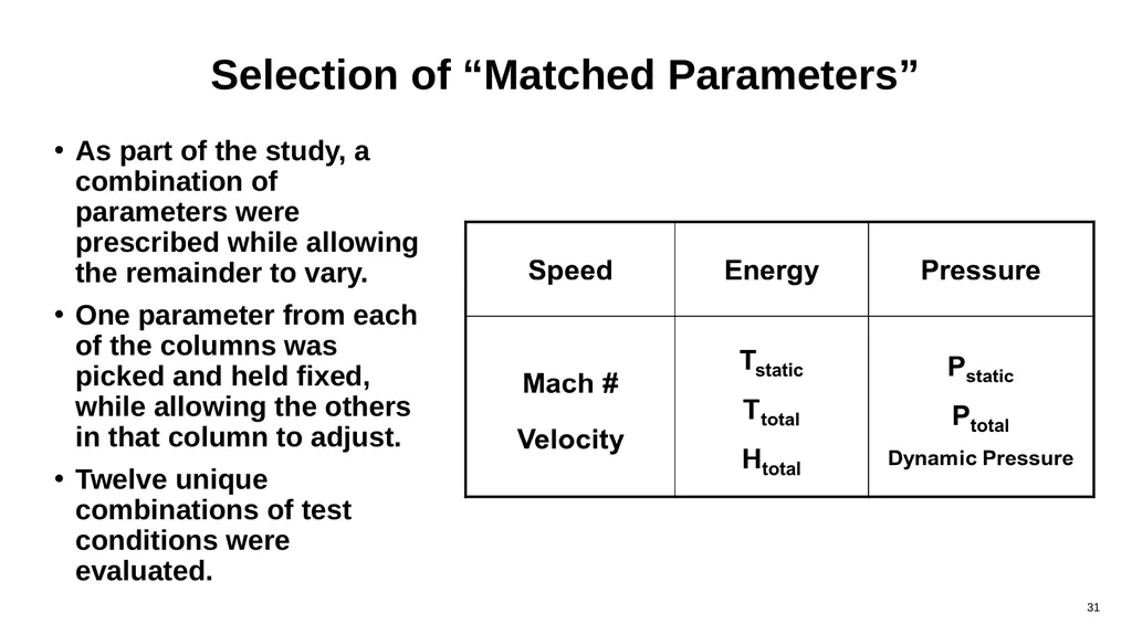
slide31. Selection of “Matched Parameters” As part of the study, a combination of parameters were prescribed while allowing the remainder to vary.
One parameter from each of the columns was picked and held fixed, while allowing the others in that column to adjust.
Twelve unique combinations of test conditions were evaluated.<br>
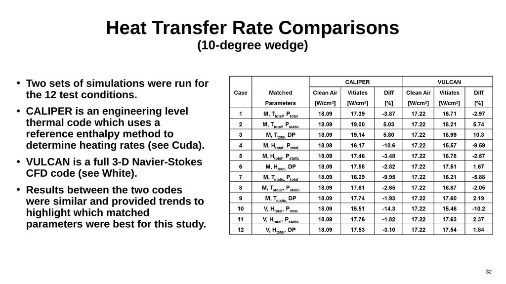
slide32. Heat Transfer Rate Comparisons (10-degree wedge) Two sets of simulations were run for the 12 test conditions.
CALIPER is an engineering level thermal code which uses a reference enthalpy method to determine heating rates (see Cuda).
VULCAN is a full 3-D Navier-Stokes CFD code (see White).
Results between the two codes were similar and provided trends to highlight which matched parameters were best for this study.<br>
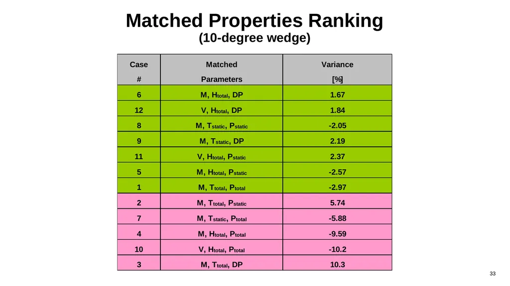
slide33. Matched Properties Ranking (10-degree wedge)<br>
slide34. What conditions are best to match? As illustrated in the previous example which focused on an engine test, seven different combinations matched closely. In general, most high-speed flight research efforts seek to match enthalpy, dynamic pressure, and Mach number.
In addition to matching the flow conditions, other combinations of variables which are relevant to the airframe should be considered.
For low-speed aerodynamic tests, Reynolds number and dynamic pressure are important parameters.
For reentry problems concerned with surface ablation, heat flux and shear stress are important considerations.
As part of any analytical effort using wind tunnel data, it is essential to determine which set of variables are best to match so that a test gas over a wind tunnel model will behave like atmospheric air over a flight article.<br>
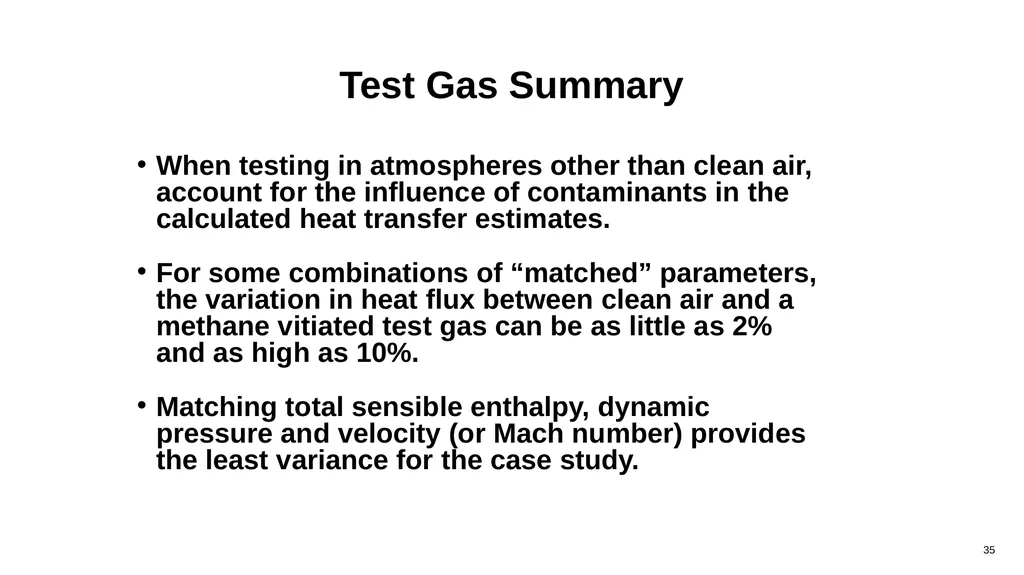
slide35. Test Gas Summary When testing in atmospheres other than clean air, account for the influence of contaminants in the calculated heat transfer estimates.
For some combinations of “matched” parameters, the variation in heat flux between clean air and a methane vitiated test gas can be as little as 2% and as high as 10%.
Matching total sensible enthalpy, dynamic pressure and velocity (or Mach number) provides the least variance for the case study.<br>
slide36. Example: Hyper-X<br>
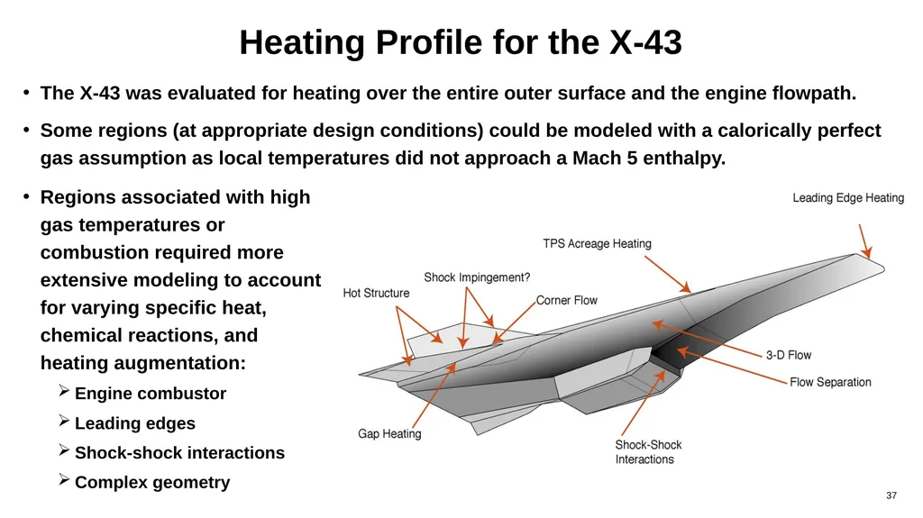
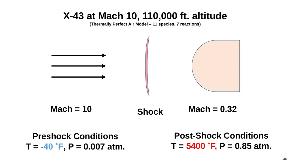
slide37. Heating Profile for the X-43 Regions associated with high gas temperatures or combustion required more extensive modeling to account for varying specific heat, chemical reactions, and heating augmentation:
Engine combustor
Leading edges
Shock-shock interactions
Complex geometry The X-43 was evaluated for heating over the entire outer surface and the engine flowpath.
Some regions (at appropriate design conditions) could be modeled with a calorically perfect gas assumption as local temperatures did not approach a Mach 5 enthalpy.<br>
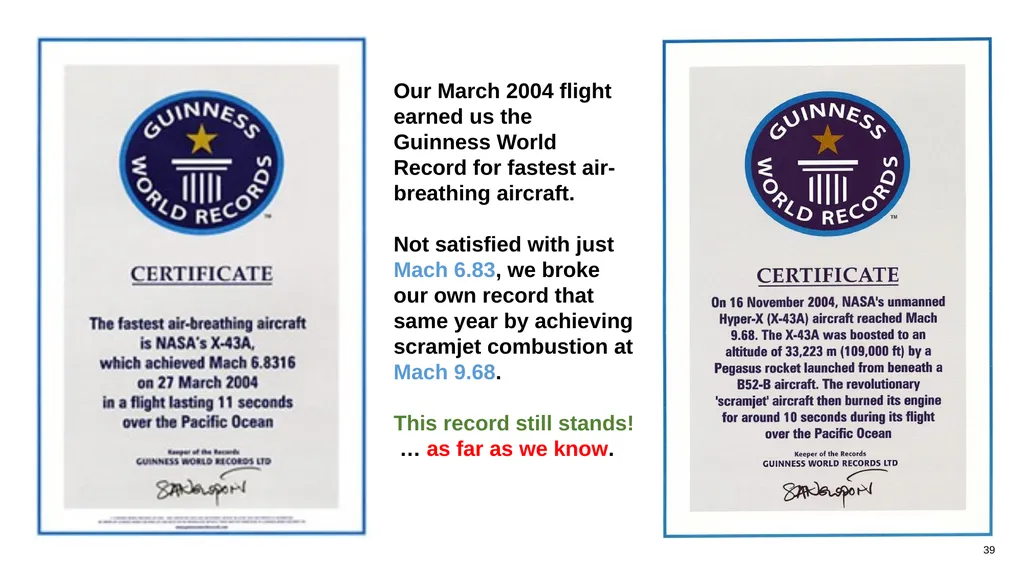
slide39. Our March 2004 flight earned us the Guinness World Record for fastest air-breathing aircraft.
Not satisfied with just Mach 6.83, we broke our own record that same year by achieving scramjet combustion at Mach 9.68.
This record still stands!
… as far as we know.<br>
slide40. References U.S. Standard Atmosphere, 1976, NOAA, NASA, USAF, Washington D.C., October 1975.
Dennis R. Jenkins, X-15, Extending the Frontiers of Flight, NASA SP-2007-562, p 166.
NACA Report 1135, Equations, Tables, and Charts for Compressible Flow, by AMES Research Staff, 1953.
Cuda, V., “Stagnation Point Heating Loads for the Hyper-X Vehicle”, Hyper-X Mach 10 Design Notice 99-004.
Cuda, V., “The CALIPER Code,” Technical Note 08-508, January 28, 2008.
Cuda, V. and Gaffney, R. I., Jr., “Analysis of the Effects of Vitiates on Surface Heat Flux in Ground Tests of Hypersonic Vehicles,” Presented at the 55th JANNAF Propulsion Meeting etc, May 12-16, 2008, Newton Massachusetts.
McBride, B. J., Zehe, M. J., and Gordon, S., “NASA Glenn Coefficients for Calculating Thermodynamic Properties of Individual Species,” NAA/TP-2002-211556, September 2002.
Prabhu, R. K. and Erickson, W. D., “A Rapid Method for the Computation of Equilibrium Chemical Composition of Air to 15,000 K”, NAS Technical Paper 2792, March 1988.
White, J. A. and Morrison, J. H., “A Pseudo-Temporal Multi-Grid Relaxation Scheme for Solving the Parabolized Navier-Stokes,” AIAA paper 99-3360, June, 1999.<br>
slide2. Important Questions Integrated Approach For Hypersonic Vehicle Designs
What constitutes a complete research effort?
How do various Systems Disciplines interact?
Air Models
How is air defined?
How many species are required to accurately model air?
Ideal and Real Gases
What is a calorically perfect gas? A thermally perfect gas?
When do these assumptions fail?
When are nonequilibrium effects important?
Test Gases
Do wind tunnel test gases behave the same as clean air?
When matching wind tunnel conditions to flight conditions, which properties are the best choice for heat transfer results?
Example<br>
slide3. Hypersonic Scramjet Flowpath Development Flight Test Ground Test Simulation Verification of flight bridging
Data for analytical model development Design database and trade studies. Test interpretation and analysis of off-trajectory points Quantification of facility/model effects Facility/model configuration assessment and gauge placement. Data consistency and test interpretation Verification of computational methodology.
Data for analytical model development. Design database and parametric testing
Viable scramjet operation that meets objectives<br>
slide4. Integrated Systems Design Approach<br>
slide5. Air<br>
slide6. Air Standards In chemistry, the International Union of Pure and Applied Chemistry (IUPAC) established standard temperature and pressure (abbreviated as STP) as a temperature of 273.15 K (0 °C, 32 °F) and an absolute pressure of exactly 100,000 Pa (1 bar, 14.5 psi, 0.9869 atmosphere).
The National Institute of Standards and Technology (NIST) uses a temperature of 20 °C (293.15 K, 68 °F) and an absolute pressure of 1 atmosphere (14.696 psi, 101.325 kPa). This standard is also called normal temperature and pressure (abbreviated as NTP).<br>
slide7. Air Models U.S. Standard Atmosphere (NASA TM-X-74335, 1976)
Releases were made in 1958, 1962, 1966 supplement, and 1976.
It is a relatively simple model and is easy to implement.
There are minimal differences between the two major releases (1962 and 1976) below altitudes of 100 km.
NASA Earth Global Reference Atmospheric Model (Earth-GRAM 2016)
Accounts for geographical variability and seasonal variability.
More stringent design criteria as environment is tuned to a specific time of year and geographical location.
Military Standard (MIL-HDBK-310, 23 June 1997)
Extensive description of various climates including temperature, humidity, rain, wind, ice, hail, snow load, sand, dust, and freeze-thaw conditions.
Includes 1, 5, 10, and 20% temperature and pressure extremes vs. altitude which may end up as part of a design requirement in hardware development.
The 1976 U.S. Standard Atmosphere is incorporated in most of the engineering and CFD codes at NASA/LaRC.<br>
slide8. Atmospheric Constituents (1976 U.S. Atmosphere)<br>
slide9. U.S. Standard Atmosphere 1976 air is a clean, dry, perfect gas mixture
specific heat ratio (g) = 1.40
molecular weight = 28.9644 [kmoles/kg] from sea level to 85.5 km
top three constituents account for 99.95% of the mass:
N2 75.5202 %
O2 23.1421 %
Ar 1.2882 %
standard sea level (SSL) condition:
P = 14.696 lbf/in2 [101,325 Pa)
T = 59 °F [15 °C]
properties are provided for air up to 1000 kilometers in altitude<br>
slide10. Modeled Species In addition to different atmospheric models existing, an assumption of the number of species that are needed to accurately represent air will be required for computational models.
The most basic air model can be represented by a single species (a composite of multiple species). The “air” 1-species model is a nonreacting model.
A 2-species model of N2 and O2 is almost identical to a 1-species “air” model.
A 5-species reacting model (N2, O2, N, O, NO) accounts for diatomic gas decomposition of the 2-species model.
For the 2- and 5-species models, Argon is excluded because it only accounts for 1% of the gas at sea level, and it does not react at moderate temperatures (less than 1% of Ar is converted to Ar+ below 20000 R).
An 11-species model (N2, O2, N, O, NO, Ar, NO+, e-, N+, O+, Ar+) is often used to account for ionization that occurs at higher temperatures (over 10,000 R, see Prabhu and Erickson).
Note: CFD simulation speed is greatly reduced as the number of species increases.<br>
slide11. Air Models in Selected NASA/LaRC Codes In general, codes can accommodate any combination of constituents and reactions. The user needs to supply the properties of the species and the various reactions expected for the flow. Some common selections include:
Selected CFD codes at LaRC have the following options:
One species (Air), nonreacting.
Four species (N2, O2, CO2, Ar), nonreacting.
Five species (N2, O2, N, O, NO), five reactions.
Ten species (N2, O2, N, O, NO, N2O, NO2, CO, CO2, Ar), sixteen reactions.
Eleven species (N2, O2, N, O, NO, Ar, NO+, e-, N+, O+, Ar+), seven reactions.
STAGHEAT (Cuda - 1999) - Leading edge engineering code has two options:
One species (Air), nonreacting.
Eleven species (N2, O2, N, O, NO, Ar, NO+, e-, N+, O+, Ar+), seven reactions.<br>
slide12. N2 and O2 Decomposition vs. Temperature (5 species, reacting air model) Note: The total mass fraction is less than 1.000 as minor species are discarded from this model. One approach to account for the total mass is to add the mass fractions of the remaining species to N2 as it doesn’t participate in reactions with fuel studies.<br>
slide13. Air Molecular Weight vs. Altitude For flight profiles above 85.5 km (typical of reentry from space), the constituents for air change.
The higher the altitude, the lower the molecular weight of the gas.
Some of the chemical processes that contribute to this decrease include:
Strong absorption of UV solar radiation by N2 and O2, resulting in a significant atmospheric temperature rise (600 to 3000 F depending upon solar activity)
Dissociation of molecular oxygen
Molecular diffusion
At 1000 km, which is the region where helium dominates, the molecular weight approaches a value near 4.<br>
slide14. Atmosphere-Space Interface 85.5 km is the last altitude within the 1976 US Standard Atmosphere where the molecular weight of each gas species remains the same as that of sea level.
The Fédération Aéronautique Internationale set the beginning of space at 100 km (62.14 miles). This altitude is known as the “Kármán line.”
The highest altitude achieved by the X-15 was 67.08 miles on August 22, 1963. Aerodynamic controls were effective up to 150,000 feet (28.41 miles). “Reaction control system is needed when dynamic pressure is less than 50 lbf/ft2” rule of thumb – N. Armstrong, see Jenkins
400,000 ft is the nominal entry point for a spacecraft simulation to begin a heating assessment.
A low earth orbit is about 160 km (99.42 miles). At this altitude, the orbital period is 88 minutes.<br>
slide15. Real Gases and Compressible Flows<br>
slide16. Photograph of 4X4 Supersonic Pressure Tunnel staff taken in the 1950s, with 'human computers' in the front row: L. Doris Barron; Amy Swann; Virginia Finch, Peggy White; Jean Pond; Evalyn Wells; Mary Korycinski; Doris Blanchard; Phyllis Henry; Mary Jackson. 4x4 Supersonic Pressure Tunnel<br>
slide17. How was the Ideal Gas Law was Discovered? Based on four variables, there are six different possible trends that can be established for two properties while holding the other two constant (varying two of P, V, T, n while holding the other two constant; note that the gas constant, R, does not vary). Four of these six trends were named. After the named trends were discovered, the comprehensive ideal gas law expression was developed which satisfies each of the original studies.
P – Absolute Pressure [Pa]
V – Volume [m3]
T – Absolute Temperature [K]
n – number of moles [moles]
R – Gas Constant 8.314 [J/moles-K]<br>
slide18. The Universal Gas Constant (R*) (and some helpful conversions) Metric System
8.3143 J/mol-K
0.08206 atm-m3/kmol-K
0.08206 atm-L/mol-K
1.986 cal/mol-K
82.06 atm-cm3/mol-K
8314.3 J/kmol-K
8314.3 kg-m2/s2-kmol-K
8314.3 m3-Pa/kmol-K
8.314E+07 erg/mol-K
English System
0.7302 atm-ft3/lbmol-R
1.986 Btu/lbmol-R
10.73 ft3-lbf/in2-lbmol-R
1545.33 ft-lbf/lbmol-R Gas constant for air (recast in alternate English units):
Rair = R* x Gc = 53.35 [ft-lbf/lbm-R] x 32.174 [lbm-ft/lbf-sec2]
= 1716.5 [ft2/sec2-R]
Rair = R* / Joule = 53.35 [ft-lbf/lbm-R] / 778.17 [ft-lbf/BTU]
= 0.0686 [BTU/lbm-R] Note: according to one source, there are over 900 unique forms to represent R*. Some forms of the universal gas constant (See note below)<br>
slide19. Forms of the Ideal Gas Law<br>
slide20. Terminology A calorically perfect gas implies that the specific heats and the gas constant are not functions of temperature.
A thermally perfect gas implies that the specific heats are functions of temperature only.
A calorically and thermally imperfect gas (also known as a real gas) implies that the specific heats are functions of both temperature and pressure.
A perfect gas implies that the equation of state, P=rRT, is valid. Since this relation does not hold for an imperfect gas, an alternate equation of state is required.
An adiabatic constraint requires that the flow process must take place without heat transfer; equations so marked may be applied to flow across a shock wave.
An isentropic constraint requires that the flow process is both reversible and adiabatic; equations so marked may not be applied to flow across a shock wave.
Note: Some researchers use the terms “thermally perfect gas” and “real gas” synonymously. In this presentation, the two terms will be treated as satisfying two different sets of conditions. * Individual species gas constants (R) do not change, but the overall mixture gas constant (Rmix) will change when chemical reactions occur.<br>
slide21. Compressible Flow Governing Equations Thermally Perfect Solution Approach
Guess total temperature
Evaluate cp = cp (T) via gas tables (see McBride)
Determine total enthalpy
Test for total enthalpy convergence
Adjust total temperature until convergence Calorically Perfect Solution Approach
Noniterative
Solve for governing equations using static conditions and constant property specific heats Relationship between total and static properties *numbers in parentheses refer to equations as found in NACA Report 1135<br>
slide22. Compressible Flow Governing Equations Continued (equations in brackets from NACA Report 1135) Thermally perfect solution approach for normal and oblique shock crossings<br>
slide23. When do Variable Properties and Chemical Effects Become Important? Consider the case of stagnation heating on a blunt body in atmospheric air.
Three models are illustrated:
No chemical reactions with constant specific heat
No chemical reactions with variable specific heat
Chemical reactions with variable specific heat
Above Mach 5, variable specific heat must be considered.
Above Mach 8, chemical reactions must be considered. *Note: Stagnation temperature is insensitive to dynamic pressure and leading-edge radius.<br>
slide24. Thermally Imperfect Gases (aka Real Gases) A thermally imperfect gas is defined as: Z = P/rRT where Z ≠1.000.
To model these flows, the equation of state needs to be modified to account for the influence of molecule size and internal structure.
Various models that account for real gas effects include:
Clausius
Van der Waals
Beattie-Bridgmann
Typically, real gas effects are not considered in aerodynamic simulations.
However, when working with scramjet hydrocarbon combustion, real gas effects may become important.<br>
slide25. Additional Considerations Nonequilibrium Flows
Thermally Imperfect Gases
Regions Requiring Special Attention<br>
slide26. Nonequilibrium Temperature and Chemistry<br>
slide27. Ground Test Gases<br>
slide28. Test Gases are Different from Atmospheric Air In order to generate the desired high enthalpy conditions associated with hypersonic flight, various methods are used to heat the air.
Each test gas must be evaluated for the various contaminants (vitiates) that are generated to produce the desired flow conditions.
Methane combustion, as used in the 8-Ft. High Temperature Tunnel, produces H2O and CO2 byproducts which change the chemical makeup of the air.
When trying to compare atmospheric air to a test gas, compromises will be unavoidable when matching test conditions.<br>
slide29. Baseline Case (clean air) To support a proposed engine test, consider a Mach 5, dynamic pressure of 2400 lbf/ft2 flight condition. It is desired to know what the heating rate will be for a flat plate with a 10-degree incline to the flow (see Cuda and Gaffney, 2008).
The goal is to determine which parameters are the best to match so that the heating rate of the panel in the wind tunnel will closely represent the same heating rate of the panel if it were flown in clean air.<br>
slide30. Gas Model Mole Fractions For the baseline case, clean air (N2, O2, Ar) was heated via methane (CH4) combustion to achieve the required flight enthalpy.
The products of combustion (CO2, H2O) contaminated the clean air.
Oxygen (O2) was reintroduced to bring the test gas up to the pretest clean air oxygen concentration. This is typically done for combustion tests.
With the addition of the vitiates (CO2, H2O) and the added O2, the resultant gas had a lower concentration of N2.
It was shown that by changing the gas composition, a different heating profile resulted for the airframe. *8-Ft. HTT Test Run T162R20<br>
slide31. Selection of “Matched Parameters” As part of the study, a combination of parameters were prescribed while allowing the remainder to vary.
One parameter from each of the columns was picked and held fixed, while allowing the others in that column to adjust.
Twelve unique combinations of test conditions were evaluated.<br>
slide32. Heat Transfer Rate Comparisons (10-degree wedge) Two sets of simulations were run for the 12 test conditions.
CALIPER is an engineering level thermal code which uses a reference enthalpy method to determine heating rates (see Cuda).
VULCAN is a full 3-D Navier-Stokes CFD code (see White).
Results between the two codes were similar and provided trends to highlight which matched parameters were best for this study.<br>
slide33. Matched Properties Ranking (10-degree wedge)<br>
slide34. What conditions are best to match? As illustrated in the previous example which focused on an engine test, seven different combinations matched closely. In general, most high-speed flight research efforts seek to match enthalpy, dynamic pressure, and Mach number.
In addition to matching the flow conditions, other combinations of variables which are relevant to the airframe should be considered.
For low-speed aerodynamic tests, Reynolds number and dynamic pressure are important parameters.
For reentry problems concerned with surface ablation, heat flux and shear stress are important considerations.
As part of any analytical effort using wind tunnel data, it is essential to determine which set of variables are best to match so that a test gas over a wind tunnel model will behave like atmospheric air over a flight article.<br>
slide35. Test Gas Summary When testing in atmospheres other than clean air, account for the influence of contaminants in the calculated heat transfer estimates.
For some combinations of “matched” parameters, the variation in heat flux between clean air and a methane vitiated test gas can be as little as 2% and as high as 10%.
Matching total sensible enthalpy, dynamic pressure and velocity (or Mach number) provides the least variance for the case study.<br>
slide36. Example: Hyper-X<br>
slide37. Heating Profile for the X-43 Regions associated with high gas temperatures or combustion required more extensive modeling to account for varying specific heat, chemical reactions, and heating augmentation:
Engine combustor
Leading edges
Shock-shock interactions
Complex geometry The X-43 was evaluated for heating over the entire outer surface and the engine flowpath.
Some regions (at appropriate design conditions) could be modeled with a calorically perfect gas assumption as local temperatures did not approach a Mach 5 enthalpy.<br>
slide39. Our March 2004 flight earned us the Guinness World Record for fastest air-breathing aircraft.
Not satisfied with just Mach 6.83, we broke our own record that same year by achieving scramjet combustion at Mach 9.68.
This record still stands!
… as far as we know.<br>
slide40. References U.S. Standard Atmosphere, 1976, NOAA, NASA, USAF, Washington D.C., October 1975.
Dennis R. Jenkins, X-15, Extending the Frontiers of Flight, NASA SP-2007-562, p 166.
NACA Report 1135, Equations, Tables, and Charts for Compressible Flow, by AMES Research Staff, 1953.
Cuda, V., “Stagnation Point Heating Loads for the Hyper-X Vehicle”, Hyper-X Mach 10 Design Notice 99-004.
Cuda, V., “The CALIPER Code,” Technical Note 08-508, January 28, 2008.
Cuda, V. and Gaffney, R. I., Jr., “Analysis of the Effects of Vitiates on Surface Heat Flux in Ground Tests of Hypersonic Vehicles,” Presented at the 55th JANNAF Propulsion Meeting etc, May 12-16, 2008, Newton Massachusetts.
McBride, B. J., Zehe, M. J., and Gordon, S., “NASA Glenn Coefficients for Calculating Thermodynamic Properties of Individual Species,” NAA/TP-2002-211556, September 2002.
Prabhu, R. K. and Erickson, W. D., “A Rapid Method for the Computation of Equilibrium Chemical Composition of Air to 15,000 K”, NAS Technical Paper 2792, March 1988.
White, J. A. and Morrison, J. H., “A Pseudo-Temporal Multi-Grid Relaxation Scheme for Solving the Parabolized Navier-Stokes,” AIAA paper 99-3360, June, 1999.<br>