
Constraint Satisfaction Problems Tuomas Sandholm
AM
Published · 46 slides · 0 views
1 / 1

Description
Constraint Satisfaction Problems Tuomas Sandholm Read Chapter 6 of Russell Norvig Minor additions by Dave Touretzky Constraint satisfaction problems (CSPs) Standard search problem: state is a black box any data structure that supports
Related Topics
Share
Embed code
Download this presentation From Below
"Constraint Satisfaction Problems Tuomas Sandholm" is the property of its rightful owner. Permission is granted to download and print the materials on this website for personal, non-commercial use only, and to display it on your personal computer provided you do not modify the materials and that you retain all copyright notices contained in the materials. By downloading content from our website, you accept the terms of this agreement.
Presentation Transcript
01
Constraint Satisfaction Problems Tuomas Sandholm
Read Chapter 6 of Russell & Norvig Minor additions by Dave Touretzky<br>
Read Chapter 6 of Russell & Norvig Minor additions by Dave Touretzky<br>
02
Constraint satisfaction problems (CSPs) Standard search problem: state is a "black box“ – any data structure that supports successor function and goal test
CSP:
state is defined by variables Xi with values from domain Di
goal test is a set of constraints specifying allowable combinations of values for subsets of variables
Simple example of a formal representation language
Allows useful general-purpose algorithms with more power than standard search algorithms ‹#›<br>
state is defined by variables Xi with values from domain Di
goal test is a set of constraints specifying allowable combinations of values for subsets of variables
Simple example of a formal representation language
Allows useful general-purpose algorithms with more power than standard search algorithms ‹#›<br>
03
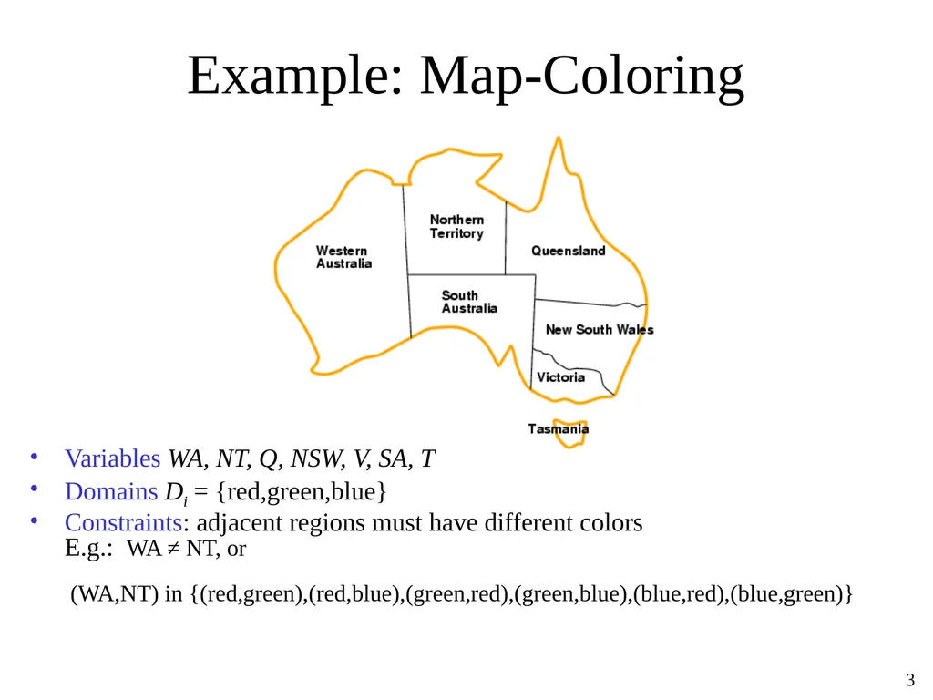
Example: Map-Coloring Variables WA, NT, Q, NSW, V, SA, T
Domains Di = {red,green,blue}
Constraints: adjacent regions must have different colors E.g.: WA ≠ NT, or (WA,NT) in {(red,green),(red,blue),(green,red),(green,blue),(blue,red),(blue,green)} ‹#›<br>
Domains Di = {red,green,blue}
Constraints: adjacent regions must have different colors E.g.: WA ≠ NT, or (WA,NT) in {(red,green),(red,blue),(green,red),(green,blue),(blue,red),(blue,green)} ‹#›<br>
04
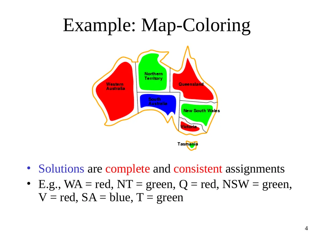
Example: Map-Coloring Solutions are complete and consistent assignments
E.g., WA = red, NT = green, Q = red, NSW = green, V = red, SA = blue, T = green ‹#›<br>
E.g., WA = red, NT = green, Q = red, NSW = green, V = red, SA = blue, T = green ‹#›<br>
05
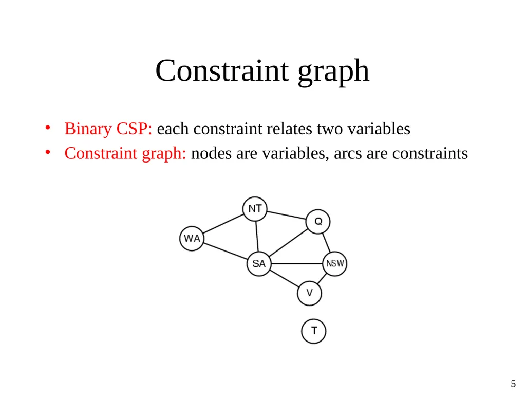
Constraint graph Binary CSP: each constraint relates two variables
Constraint graph: nodes are variables, arcs are constraints ‹#›<br>
Constraint graph: nodes are variables, arcs are constraints ‹#›<br>
06
Varieties of CSPs Discrete variables
finite domains:
n variables, domain size d → O(dn) complete assignments
E.g., Boolean CSPs, incl. Boolean satisfiability (NP-complete)
infinite domains:
integers, strings, etc.
E.g., job scheduling, variables are start/end days for each job
can’t enumerate all possible assignments, so need a constraint language, e.g., StartJob1 + 5 ≤ StartJob3
Continuous variables
E.g., start/end times for Hubble Space Telescope observations
linear constraints solvable in polynomial time by linear programming (LP) ‹#›<br>
finite domains:
n variables, domain size d → O(dn) complete assignments
E.g., Boolean CSPs, incl. Boolean satisfiability (NP-complete)
infinite domains:
integers, strings, etc.
E.g., job scheduling, variables are start/end days for each job
can’t enumerate all possible assignments, so need a constraint language, e.g., StartJob1 + 5 ≤ StartJob3
Continuous variables
E.g., start/end times for Hubble Space Telescope observations
linear constraints solvable in polynomial time by linear programming (LP) ‹#›<br>
07
Varieties of constraints Unary constraints involve a single variable,
e.g., SA ≠ green
Binary constraints involve pairs of variables,
e.g., SA ≠ WA
Higher-order constraints involve 3 or more variables,
e.g., cryptarithmetic column constraints
global constraints such as Alldiff ‹#›<br>
e.g., SA ≠ green
Binary constraints involve pairs of variables,
e.g., SA ≠ WA
Higher-order constraints involve 3 or more variables,
e.g., cryptarithmetic column constraints
global constraints such as Alldiff ‹#›<br>
08
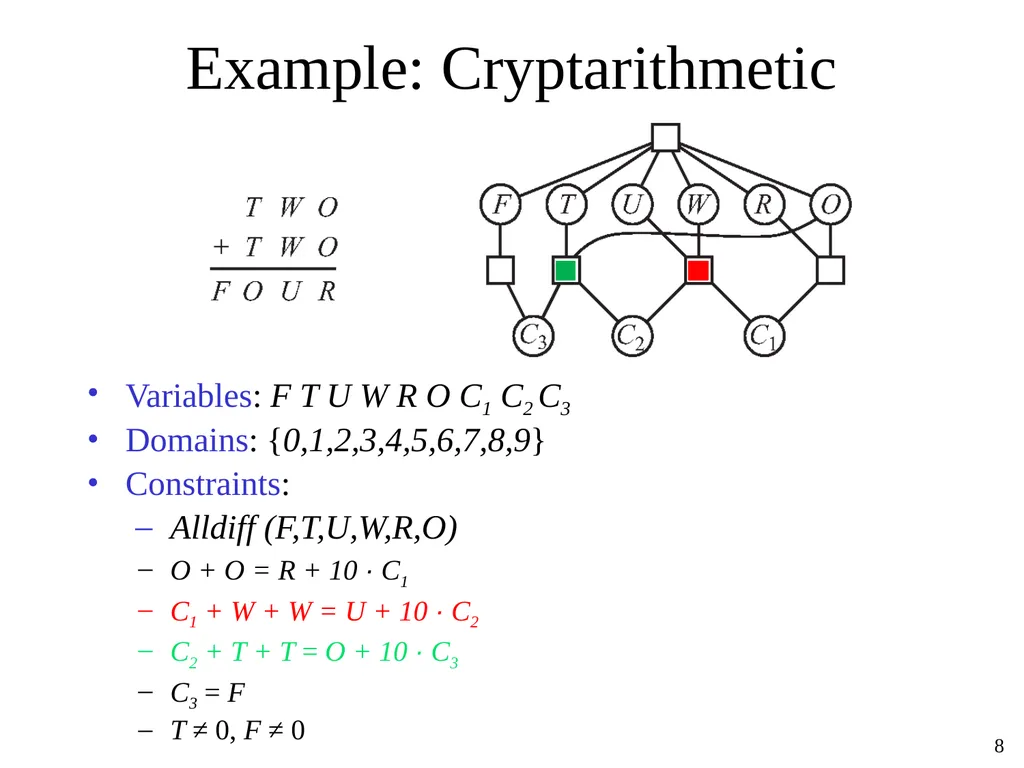
Example: Cryptarithmetic Variables: F T U W R O C1 C2 C3
Domains: {0,1,2,3,4,5,6,7,8,9}
Constraints:
Alldiff (F,T,U,W,R,O)
O + O = R + 10 · C1
C1 + W + W = U + 10 · C2
C2 + T + T = O + 10 · C3
C3 = F
T ≠ 0, F ≠ 0 ‹#›<br>
Domains: {0,1,2,3,4,5,6,7,8,9}
Constraints:
Alldiff (F,T,U,W,R,O)
O + O = R + 10 · C1
C1 + W + W = U + 10 · C2
C2 + T + T = O + 10 · C3
C3 = F
T ≠ 0, F ≠ 0 ‹#›<br>
09
Real-world CSPs Assignment problems
e.g., who teaches what class
Timetabling problems
e.g., which class is offered when and where?
Transportation scheduling Factory scheduling
Notice that many real-world problems involve real-valued variables ‹#›<br>
e.g., who teaches what class
Timetabling problems
e.g., which class is offered when and where?
Transportation scheduling Factory scheduling
Notice that many real-world problems involve real-valued variables ‹#›<br>
10
Two Kinds of CSP Inference Steps Search: pick some variables and assign values to them. Can use DFS.
Constraint propagation: use the values of some variables to reduce the set of possible values for other variables. Repeat until no further reductions are possible. ‹#›<br>
Constraint propagation: use the values of some variables to reduce the set of possible values for other variables. Repeat until no further reductions are possible. ‹#›<br>
11
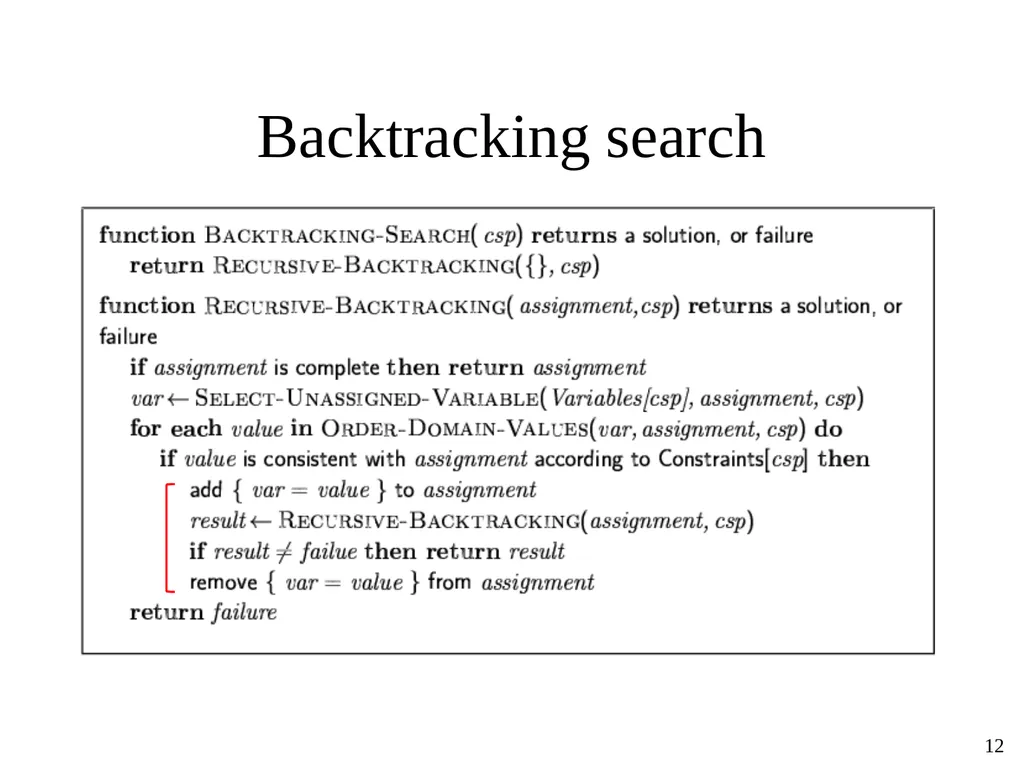
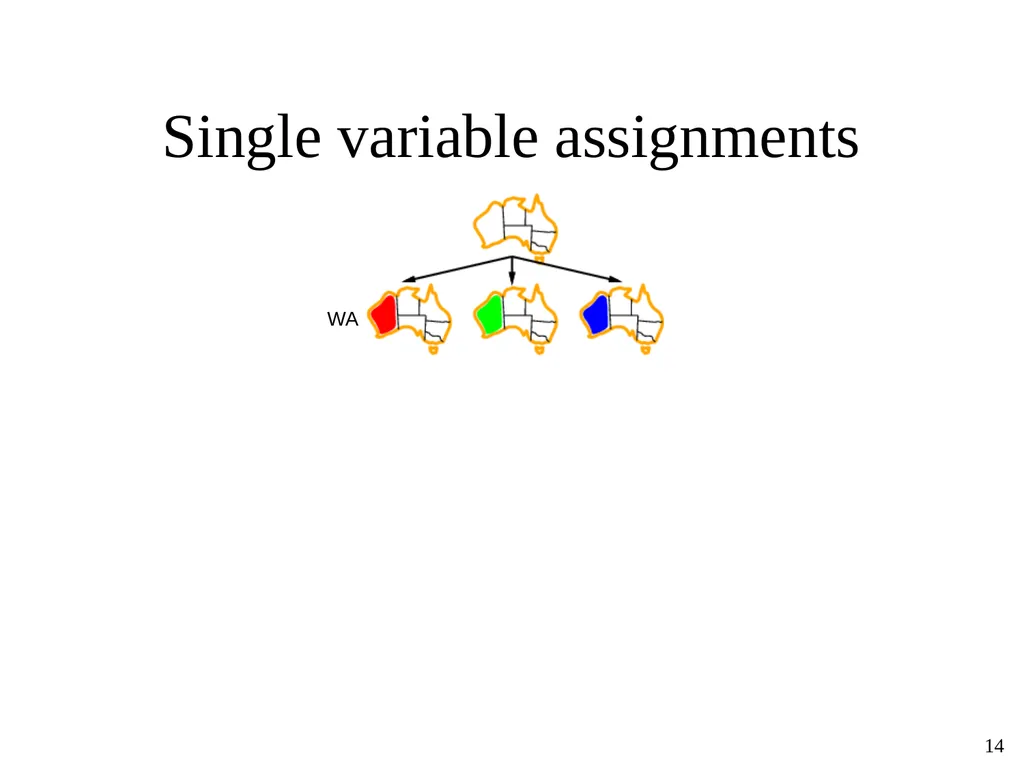
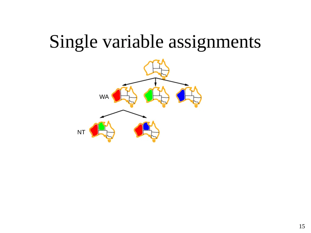
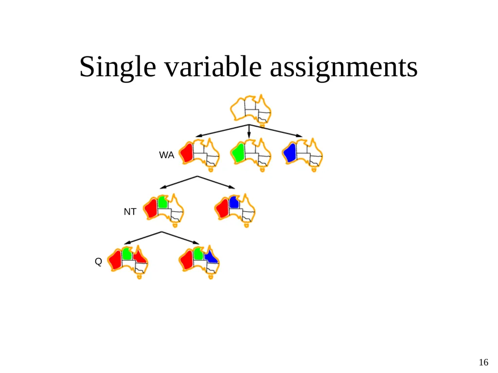
Backtracking Search Variable assignments are commutative, i.e.,
[ WA = red then NT = green ] same as [ NT = green then WA = red ]
=> Only need to consider assignments to a single variable at each node
Depth-first search for CSPs with single-variable assignments is called backtracking search
Can solve n-queens for n ≈ 25 ‹#›<br>
[ WA = red then NT = green ] same as [ NT = green then WA = red ]
=> Only need to consider assignments to a single variable at each node
Depth-first search for CSPs with single-variable assignments is called backtracking search
Can solve n-queens for n ≈ 25 ‹#›<br>
12
Backtracking search ‹#›<br>
13
Single variable assignments ‹#›<br>
14
WA Single variable assignments ‹#›<br>
15
Single variable assignments ‹#› WA NT<br>
16
Single variable assignments ‹#› WA NT Q<br>
17
Improving backtracking efficiency General-purpose methods can give huge gains in speed:
Which variable should be assigned next?
In what order should its values be tried?
Can we detect inevitable failure early? ‹#›<br>
Which variable should be assigned next?
In what order should its values be tried?
Can we detect inevitable failure early? ‹#›<br>
18
Question for the class The “most constrained” variable is the one with the fewest choices of values.
In a depth-first search, would it be better to explore assignments to the most constrained or the least constrained variable next? ‹#›<br>
In a depth-first search, would it be better to explore assignments to the most constrained or the least constrained variable next? ‹#›<br>
19
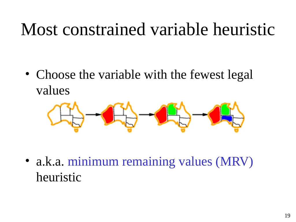
Most constrained variable heuristic Choose the variable with the fewest legal values
a.k.a. minimum remaining values (MRV) heuristic ‹#›<br>
a.k.a. minimum remaining values (MRV) heuristic ‹#›<br>
20
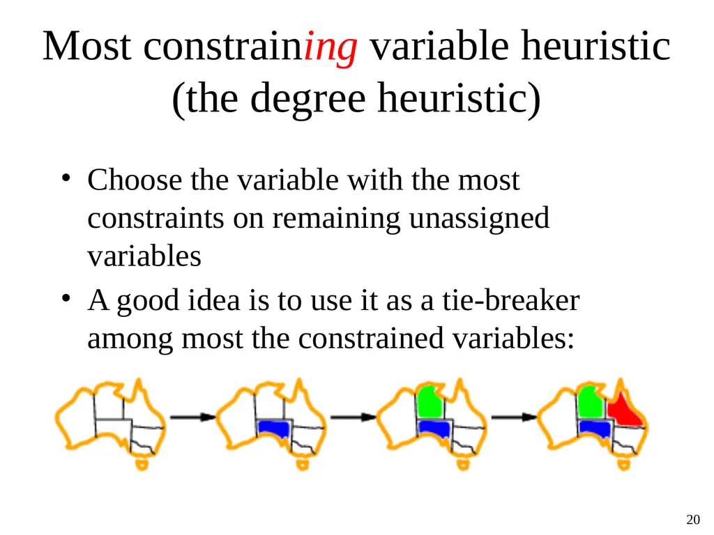
Most constraining variable heuristic
(the degree heuristic) Choose the variable with the most constraints on remaining unassigned variables
A good idea is to use it as a tie-breaker among most the constrained variables: ‹#›<br>
(the degree heuristic) Choose the variable with the most constraints on remaining unassigned variables
A good idea is to use it as a tie-breaker among most the constrained variables: ‹#›<br>
21
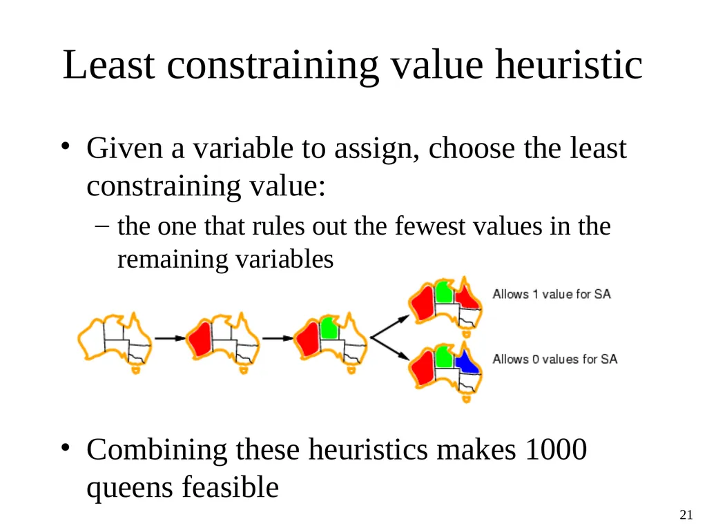
Least constraining value heuristic Given a variable to assign, choose the least constraining value:
the one that rules out the fewest values in the remaining variables
Combining these heuristics makes 1000 queens feasible ‹#›<br>
the one that rules out the fewest values in the remaining variables
Combining these heuristics makes 1000 queens feasible ‹#›<br>
22
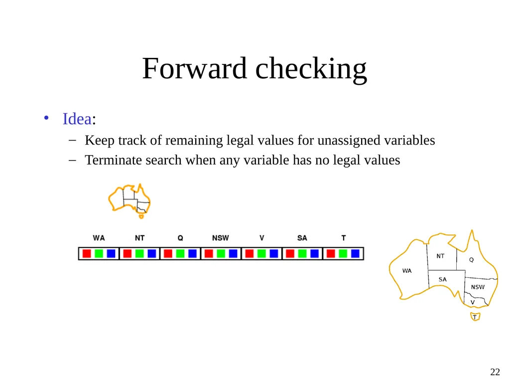
Forward checking Idea:
Keep track of remaining legal values for unassigned variables
Terminate search when any variable has no legal values ‹#›<br>
Keep track of remaining legal values for unassigned variables
Terminate search when any variable has no legal values ‹#›<br>
23
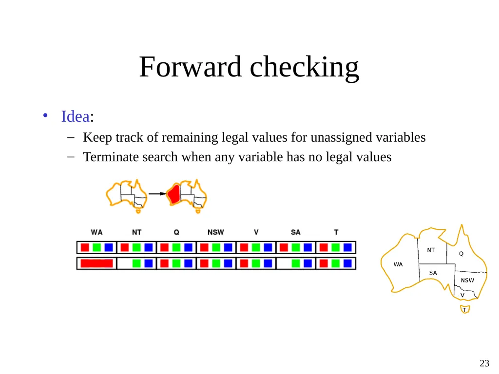
Forward checking Idea:
Keep track of remaining legal values for unassigned variables
Terminate search when any variable has no legal values ‹#›<br>
Keep track of remaining legal values for unassigned variables
Terminate search when any variable has no legal values ‹#›<br>
24
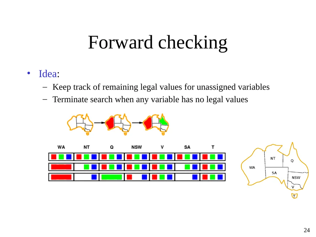
Forward checking Idea:
Keep track of remaining legal values for unassigned variables
Terminate search when any variable has no legal values ‹#›<br>
Keep track of remaining legal values for unassigned variables
Terminate search when any variable has no legal values ‹#›<br>
25
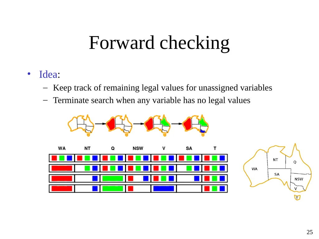
Forward checking Idea:
Keep track of remaining legal values for unassigned variables
Terminate search when any variable has no legal values ‹#›<br>
Keep track of remaining legal values for unassigned variables
Terminate search when any variable has no legal values ‹#›<br>
26
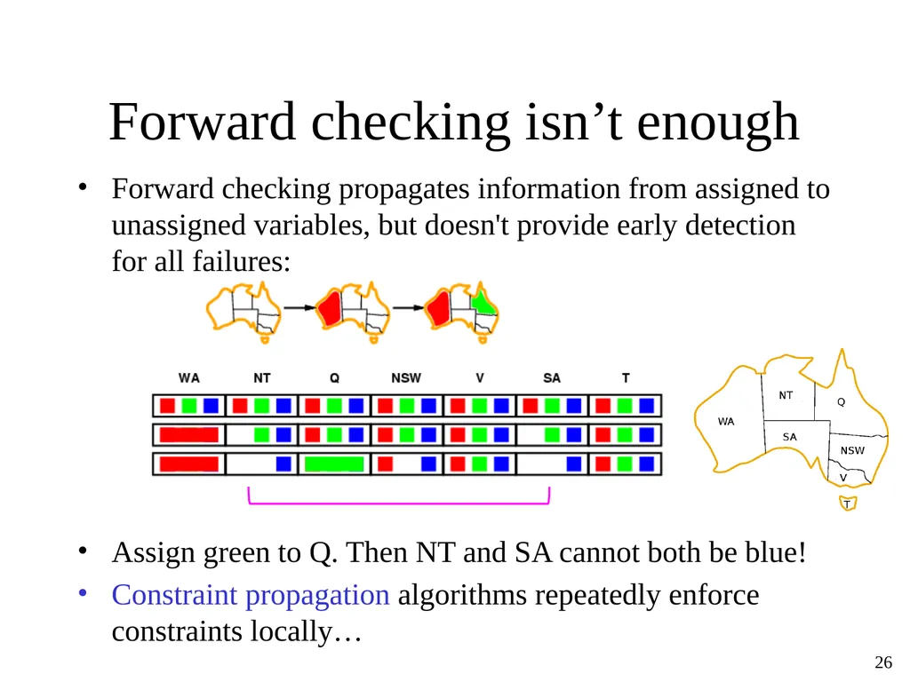
Forward checking isn’t enough Forward checking propagates information from assigned to unassigned variables, but doesn't provide early detection for all failures:
Assign green to Q. Then NT and SA cannot both be blue!
Constraint propagation algorithms repeatedly enforce constraints locally… ‹#›<br>
Assign green to Q. Then NT and SA cannot both be blue!
Constraint propagation algorithms repeatedly enforce constraints locally… ‹#›<br>
27
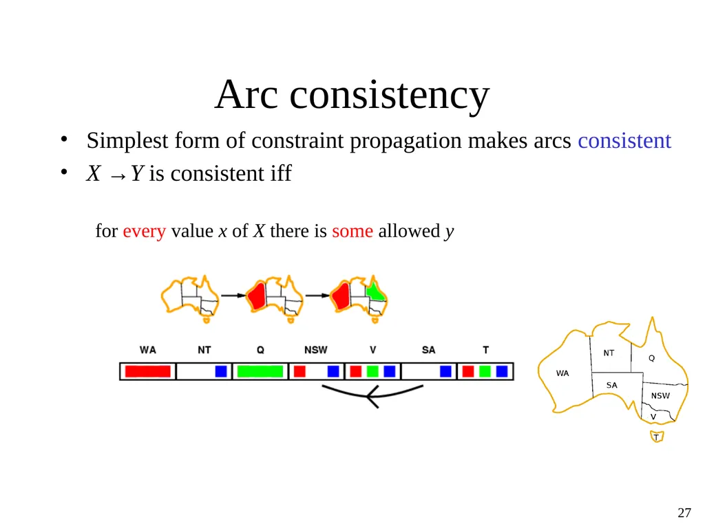
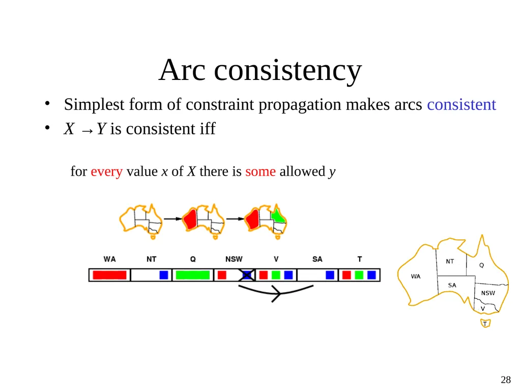
Arc consistency Simplest form of constraint propagation makes arcs consistent
X →Y is consistent iff
for every value x of X there is some allowed y ‹#›<br>
X →Y is consistent iff
for every value x of X there is some allowed y ‹#›<br>
28
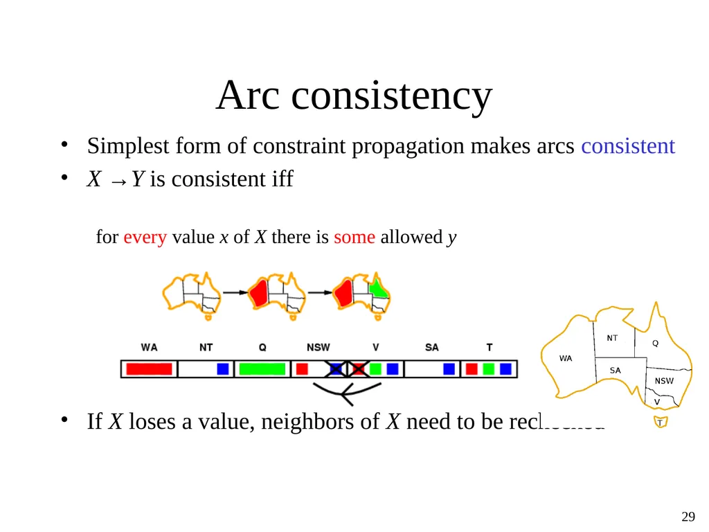
Arc consistency Simplest form of constraint propagation makes arcs consistent
X →Y is consistent iff
for every value x of X there is some allowed y ‹#›<br>
X →Y is consistent iff
for every value x of X there is some allowed y ‹#›<br>
29
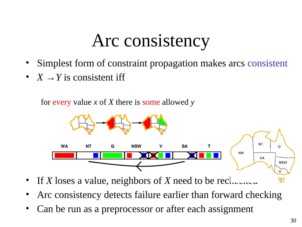
Arc consistency Simplest form of constraint propagation makes arcs consistent
X →Y is consistent iff
for every value x of X there is some allowed y
If X loses a value, neighbors of X need to be rechecked ‹#›<br>
X →Y is consistent iff
for every value x of X there is some allowed y
If X loses a value, neighbors of X need to be rechecked ‹#›<br>
30
Arc consistency Simplest form of constraint propagation makes arcs consistent
X →Y is consistent iff
for every value x of X there is some allowed y
If X loses a value, neighbors of X need to be rechecked
Arc consistency detects failure earlier than forward checking
Can be run as a preprocessor or after each assignment ‹#›<br>
X →Y is consistent iff
for every value x of X there is some allowed y
If X loses a value, neighbors of X need to be rechecked
Arc consistency detects failure earlier than forward checking
Can be run as a preprocessor or after each assignment ‹#›<br>
31
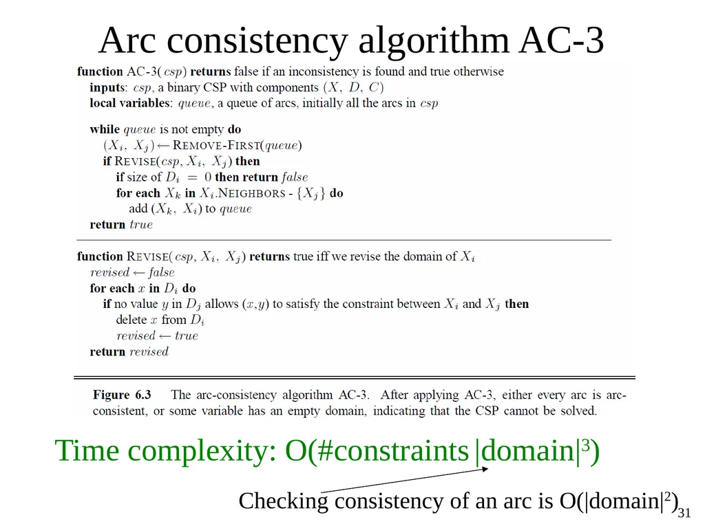
Arc consistency algorithm AC-3 Time complexity: O(#constraints |domain|3) Checking consistency of an arc is O(|domain|2) ‹#›<br>
32
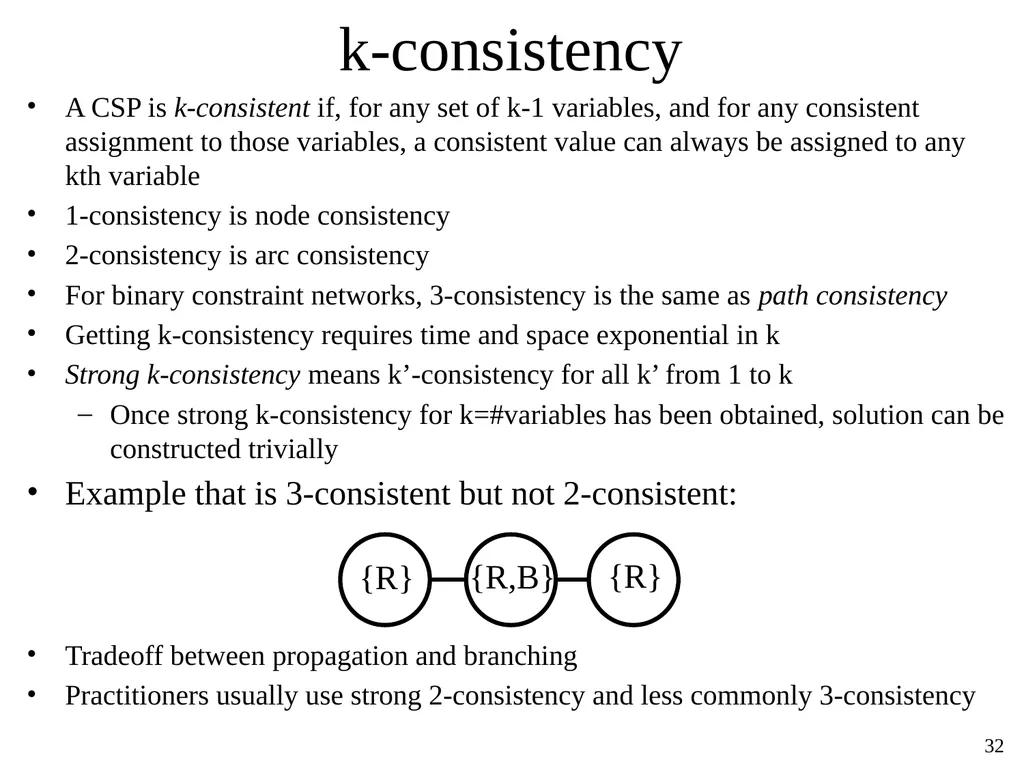
k-consistency A CSP is k-consistent if, for any set of k-1 variables, and for any consistent assignment to those variables, a consistent value can always be assigned to any kth variable
1-consistency is node consistency
2-consistency is arc consistency
For binary constraint networks, 3-consistency is the same as path consistency
Getting k-consistency requires time and space exponential in k
Strong k-consistency means k’-consistency for all k’ from 1 to k
Once strong k-consistency for k=#variables has been obtained, solution can be constructed trivially
Example that is 3-consistent but not 2-consistent:
Tradeoff between propagation and branching
Practitioners usually use strong 2-consistency and less commonly 3-consistency ‹#›<br>
1-consistency is node consistency
2-consistency is arc consistency
For binary constraint networks, 3-consistency is the same as path consistency
Getting k-consistency requires time and space exponential in k
Strong k-consistency means k’-consistency for all k’ from 1 to k
Once strong k-consistency for k=#variables has been obtained, solution can be constructed trivially
Example that is 3-consistent but not 2-consistent:
Tradeoff between propagation and branching
Practitioners usually use strong 2-consistency and less commonly 3-consistency ‹#›<br>
33
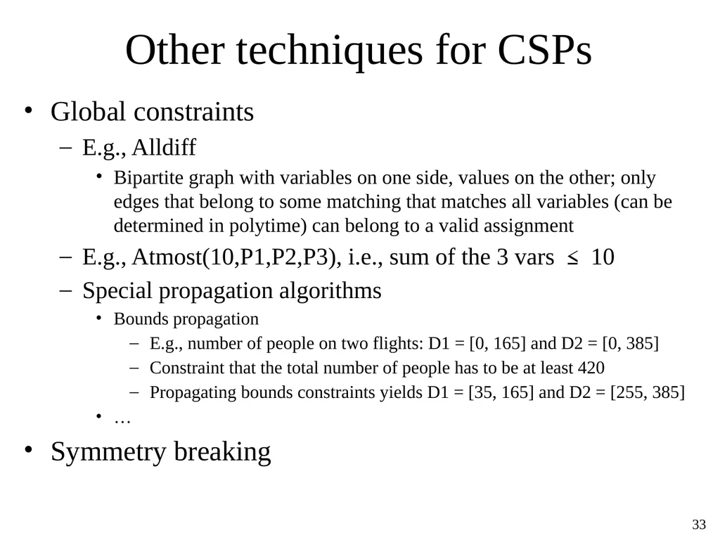
Other techniques for CSPs Global constraints
E.g., Alldiff
Bipartite graph with variables on one side, values on the other; only edges that belong to some matching that matches all variables (can be determined in polytime) can belong to a valid assignment
E.g., Atmost(10,P1,P2,P3), i.e., sum of the 3 vars ≤ 10
Special propagation algorithms
Bounds propagation
E.g., number of people on two flights: D1 = [0, 165] and D2 = [0, 385]
Constraint that the total number of people has to be at least 420
Propagating bounds constraints yields D1 = [35, 165] and D2 = [255, 385]
…
Symmetry breaking ‹#›<br>
E.g., Alldiff
Bipartite graph with variables on one side, values on the other; only edges that belong to some matching that matches all variables (can be determined in polytime) can belong to a valid assignment
E.g., Atmost(10,P1,P2,P3), i.e., sum of the 3 vars ≤ 10
Special propagation algorithms
Bounds propagation
E.g., number of people on two flights: D1 = [0, 165] and D2 = [0, 385]
Constraint that the total number of people has to be at least 420
Propagating bounds constraints yields D1 = [35, 165] and D2 = [255, 385]
…
Symmetry breaking ‹#›<br>
34
Structured CSPs<br>
35
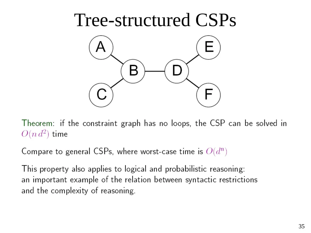
Tree-structured CSPs ‹#›<br>
36
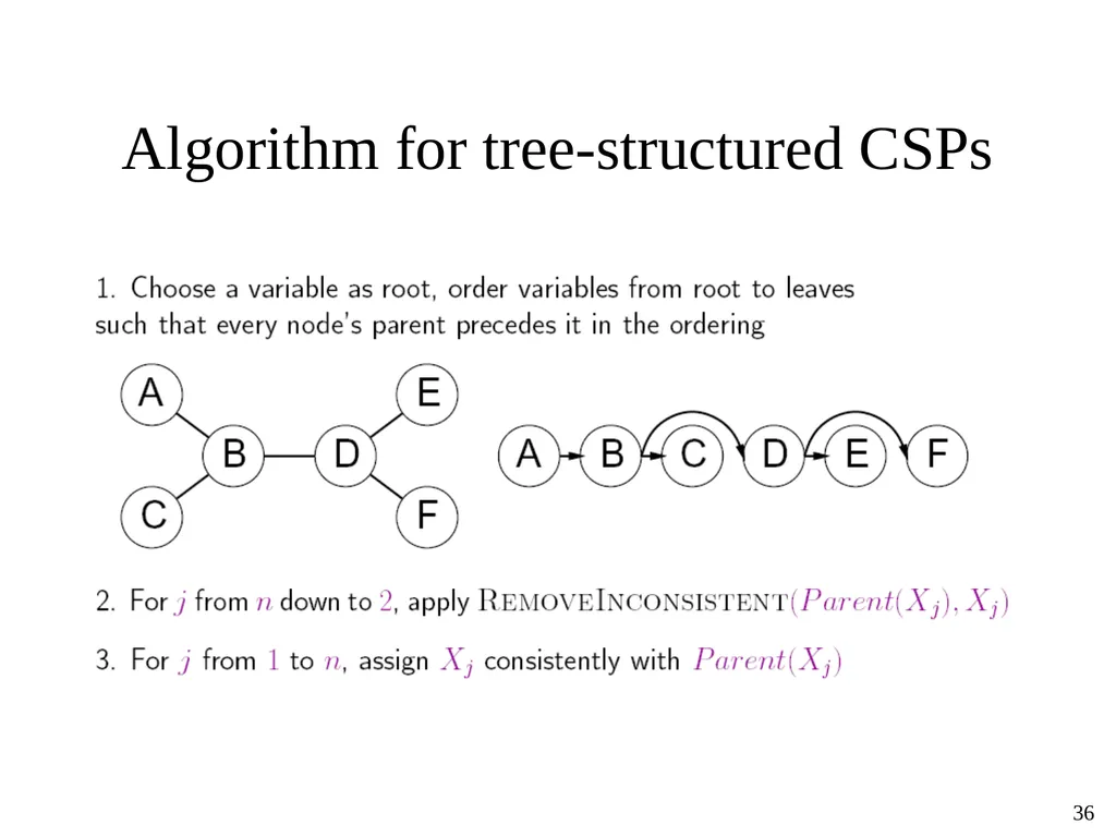
Algorithm for tree-structured CSPs ‹#›<br>
37
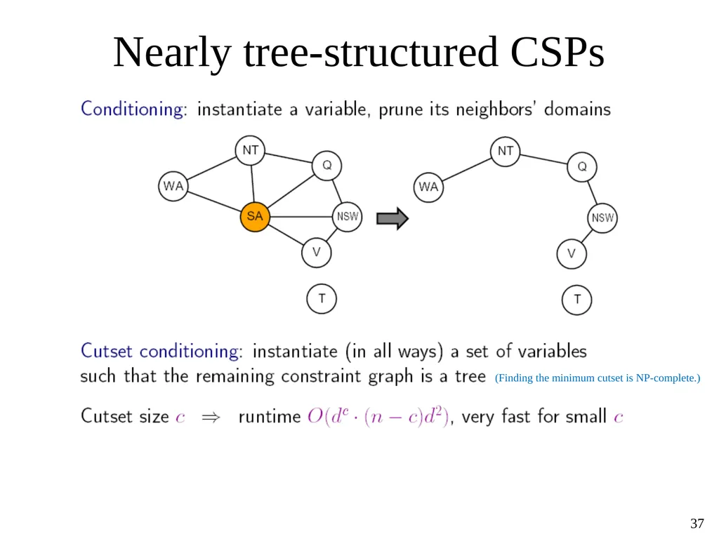
Nearly tree-structured CSPs (Finding the minimum cutset is NP-complete.) ‹#›<br>
38
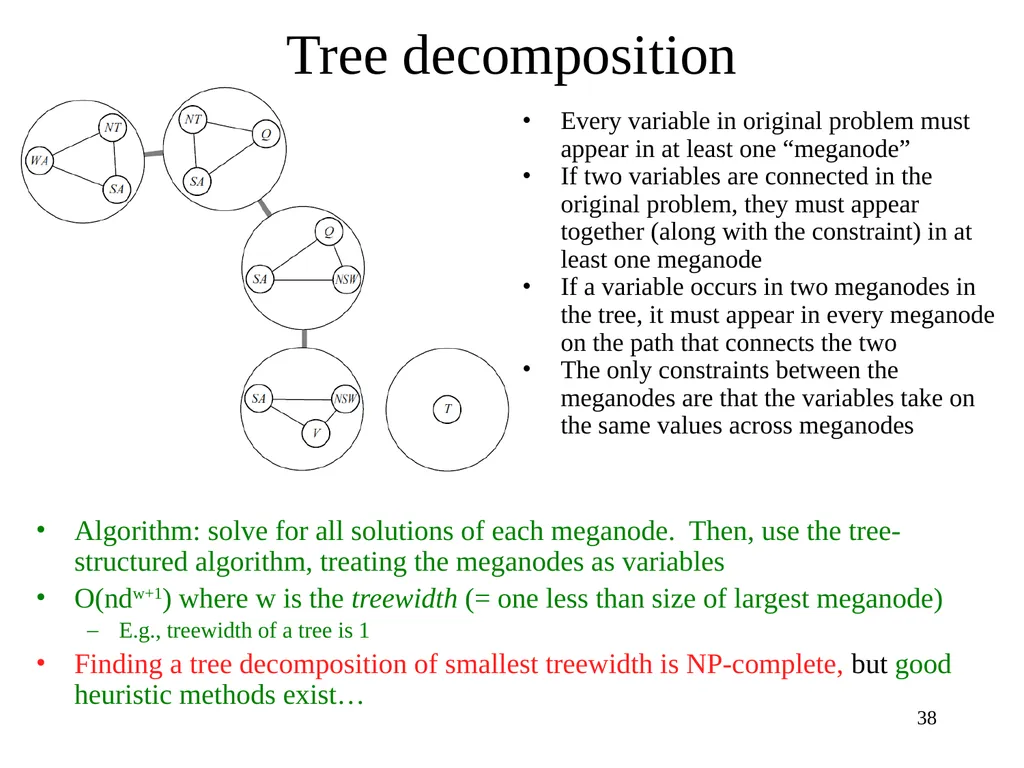
Tree decomposition Algorithm: solve for all solutions of each meganode. Then, use the tree-structured algorithm, treating the meganodes as variables
O(ndw+1) where w is the treewidth (= one less than size of largest meganode)
E.g., treewidth of a tree is 1
Finding a tree decomposition of smallest treewidth is NP-complete, but good heuristic methods exist… Every variable in original problem must appear in at least one “meganode”
If two variables are connected in the original problem, they must appear together (along with the constraint) in at least one meganode
If a variable occurs in two meganodes in the tree, it must appear in every meganode on the path that connects the two
The only constraints between the meganodes are that the variables take on the same values across meganodes ‹#›<br>
O(ndw+1) where w is the treewidth (= one less than size of largest meganode)
E.g., treewidth of a tree is 1
Finding a tree decomposition of smallest treewidth is NP-complete, but good heuristic methods exist… Every variable in original problem must appear in at least one “meganode”
If two variables are connected in the original problem, they must appear together (along with the constraint) in at least one meganode
If a variable occurs in two meganodes in the tree, it must appear in every meganode on the path that connects the two
The only constraints between the meganodes are that the variables take on the same values across meganodes ‹#›<br>
39
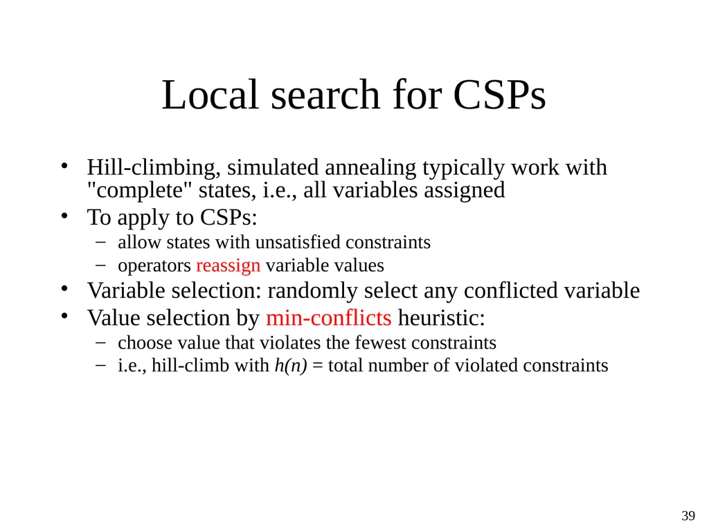
Local search for CSPs Hill-climbing, simulated annealing typically work with "complete" states, i.e., all variables assigned
To apply to CSPs:
allow states with unsatisfied constraints
operators reassign variable values
Variable selection: randomly select any conflicted variable
Value selection by min-conflicts heuristic:
choose value that violates the fewest constraints
i.e., hill-climb with h(n) = total number of violated constraints ‹#›<br>
To apply to CSPs:
allow states with unsatisfied constraints
operators reassign variable values
Variable selection: randomly select any conflicted variable
Value selection by min-conflicts heuristic:
choose value that violates the fewest constraints
i.e., hill-climb with h(n) = total number of violated constraints ‹#›<br>
40
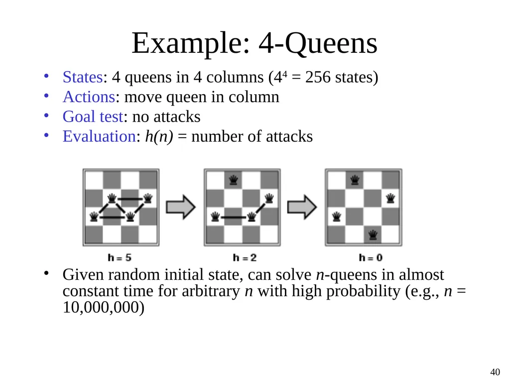
Example: 4-Queens States: 4 queens in 4 columns (44 = 256 states)
Actions: move queen in column
Goal test: no attacks
Evaluation: h(n) = number of attacks
Given random initial state, can solve n-queens in almost constant time for arbitrary n with high probability (e.g., n = 10,000,000) ‹#›<br>
Actions: move queen in column
Goal test: no attacks
Evaluation: h(n) = number of attacks
Given random initial state, can solve n-queens in almost constant time for arbitrary n with high probability (e.g., n = 10,000,000) ‹#›<br>
41
Summary CSPs are a special kind of problem:
states defined by values of a fixed set of variables
goal test defined by constraints on variable values
Backtracking = depth-first search with one variable assigned per node
Variable ordering and value selection heuristics help significantly
Forward checking prevents assignments that guarantee later failure
Constraint propagation (e.g., arc consistency) does additional work to constrain values and detect inconsistencies
Iterative min-conflicts is usually effective in practice ‹#›<br>
states defined by values of a fixed set of variables
goal test defined by constraints on variable values
Backtracking = depth-first search with one variable assigned per node
Variable ordering and value selection heuristics help significantly
Forward checking prevents assignments that guarantee later failure
Constraint propagation (e.g., arc consistency) does additional work to constrain values and detect inconsistencies
Iterative min-conflicts is usually effective in practice ‹#›<br>
42
Additional Slides (not included in this lecture) ‹#›<br>
43
Interlude Does the n-queens problem become easier or harder if some of the queens’ locations are already given and cannot be changed? ‹#›<br>
44
Hot off the press ‹#›<br>
45
Summary of the complexity of the n-queens problem The decision problem is solvable in constant time since there is a solution for all n > 3.
A witnessing solution can be constructed easily [Bell & Stevens, 2009] but note that the witness (a set of n queens) requires n log n bits to specify but this is not polynomial in the size of the input, which is only log n bits.
(The problem has often been incorrectly called NP-hard.)
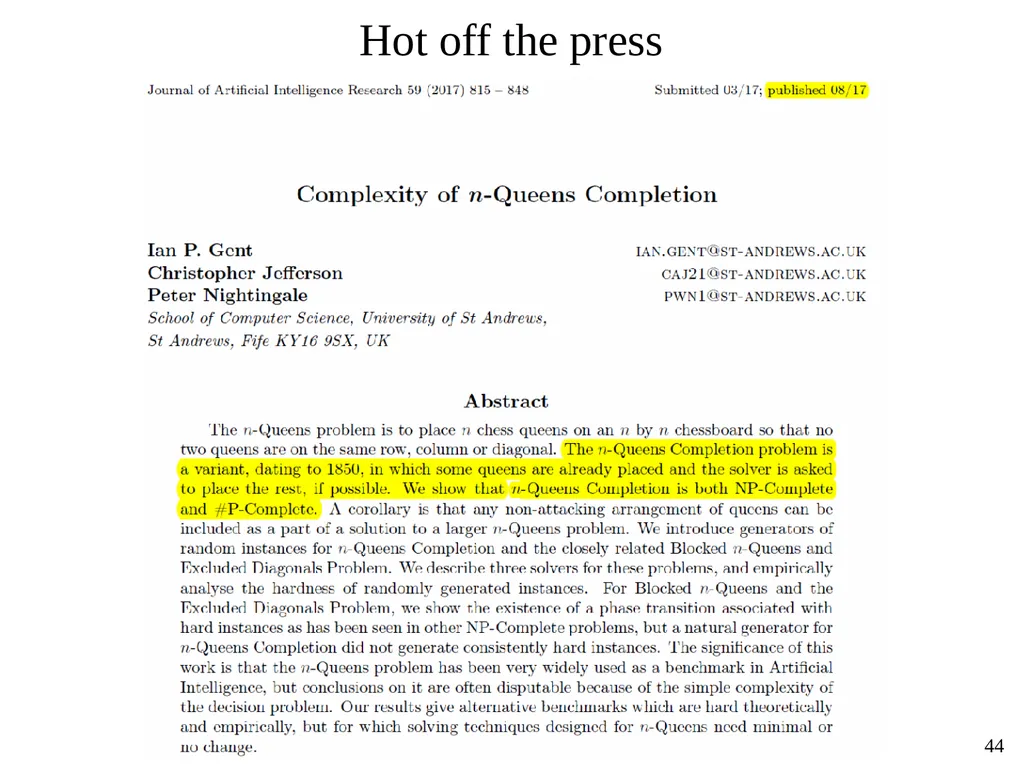
If some of the queens are already in fixed locations, the problem is NP-complete and #P-complete.
End of interlude ‹#›<br>
A witnessing solution can be constructed easily [Bell & Stevens, 2009] but note that the witness (a set of n queens) requires n log n bits to specify but this is not polynomial in the size of the input, which is only log n bits.
(The problem has often been incorrectly called NP-hard.)
If some of the queens are already in fixed locations, the problem is NP-complete and #P-complete.
End of interlude ‹#›<br>
46
Advanced topic:
State of knowledge on treewidth algorithms Determining whether treewidth of a given graph is at most k is NP-complete
In what follows, n is the number of vertices
O(sqrt(log n)) approximation of treewidth in polytime [Feige, Hajiaghayi and Lee 2008]
O(log k) approximation of treewidth in polytime [Amir 2002, Feige, Hajiaghayi and Lee 2008]
When k is any fixed constant, the graphs with treewidth k can be recognized, and a width k tree decomposition can be constructed for them, in linear time [Bodlaender 1996]
I.e., only exponential in a (large) polynomial of k
There is an algorithm that approximates the treewidth of a graph by a constant factor of 3.66, but it takes time that is exponential in the treewidth [Amir 2002]
Open question: Polynomial-time approximation scheme (PTAS) ‹#›<br>
In what follows, n is the number of vertices
O(sqrt(log n)) approximation of treewidth in polytime [Feige, Hajiaghayi and Lee 2008]
O(log k) approximation of treewidth in polytime [Amir 2002, Feige, Hajiaghayi and Lee 2008]
When k is any fixed constant, the graphs with treewidth k can be recognized, and a width k tree decomposition can be constructed for them, in linear time [Bodlaender 1996]
I.e., only exponential in a (large) polynomial of k
There is an algorithm that approximates the treewidth of a graph by a constant factor of 3.66, but it takes time that is exponential in the treewidth [Amir 2002]
Open question: Polynomial-time approximation scheme (PTAS) ‹#›<br>