04
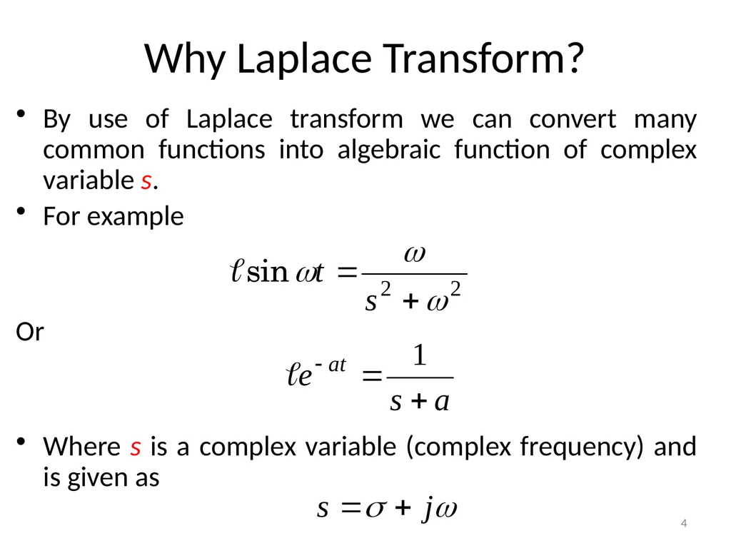
Why Laplace Transform? By use of Laplace transform we can convert many common functions into algebraic function of complex variable s.
For example
Or
Where s is a complex variable (complex frequency) and is given as 4<br>
05
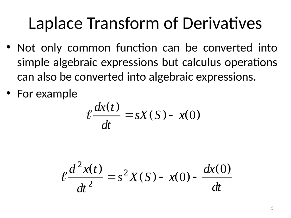
Laplace Transform of Derivatives Not only common function can be converted into simple algebraic expressions but calculus operations can also be converted into algebraic expressions.
For example 5<br>
06
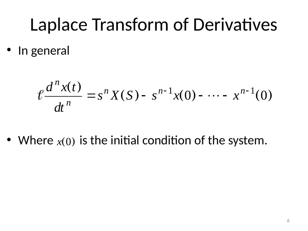
Laplace Transform of Derivatives In general
Where is the initial condition of the system. 6<br>
07
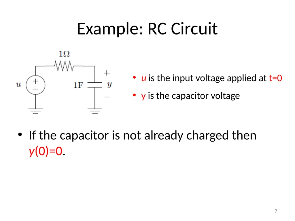
Example: RC Circuit If the capacitor is not already charged then y(0)=0. u is the input voltage applied at t=0
y is the capacitor voltage 7<br>
08
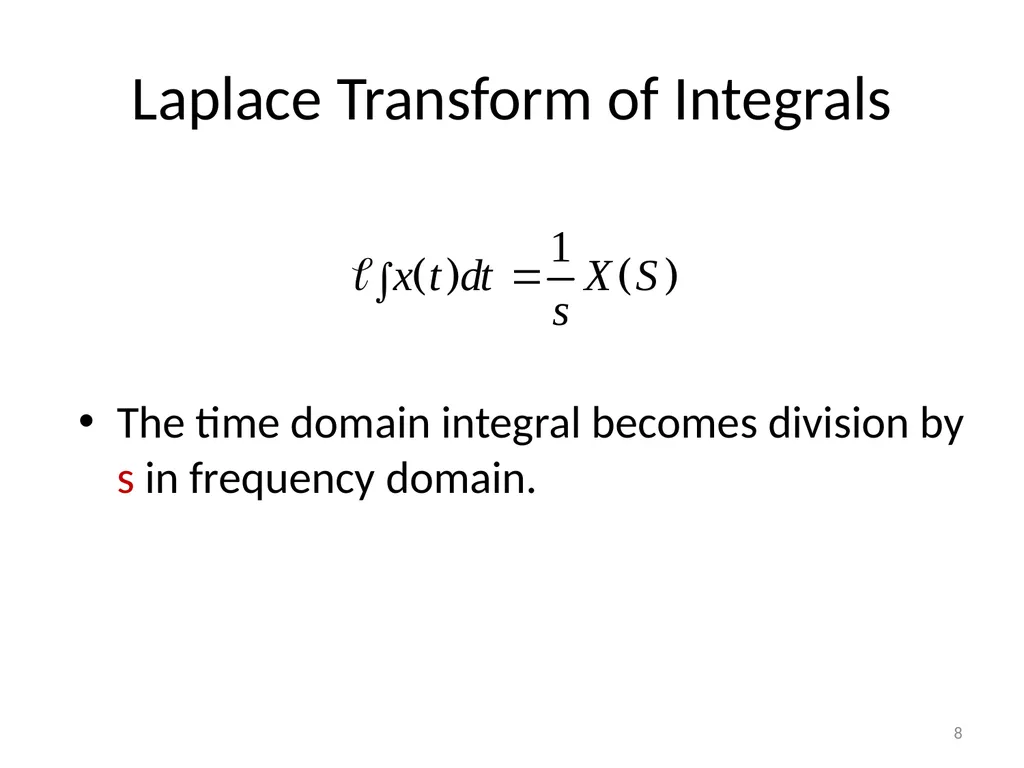
Laplace Transform of Integrals The time domain integral becomes division by s in frequency domain. 8<br>
09
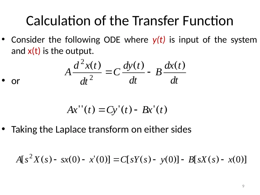
Calculation of the Transfer Function Consider the following ODE where y(t) is input of the system and x(t) is the output.
or
Taking the Laplace transform on either sides 9<br>
10
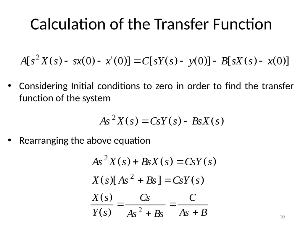
Calculation of the Transfer Function Considering Initial conditions to zero in order to find the transfer function of the system
Rearranging the above equation 10<br>
11
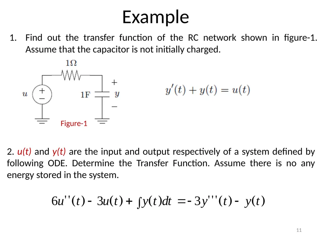
Example Find out the transfer function of the RC network shown in figure-1. Assume that the capacitor is not initially charged. 2. u(t) and y(t) are the input and output respectively of a system defined by following ODE. Determine the Transfer Function. Assume there is no any energy stored in the system. 11<br>
12
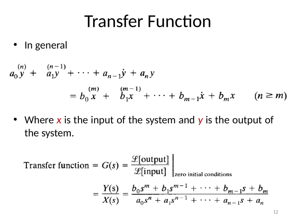
Transfer Function In general
Where x is the input of the system and y is the output of the system. 12<br>
13
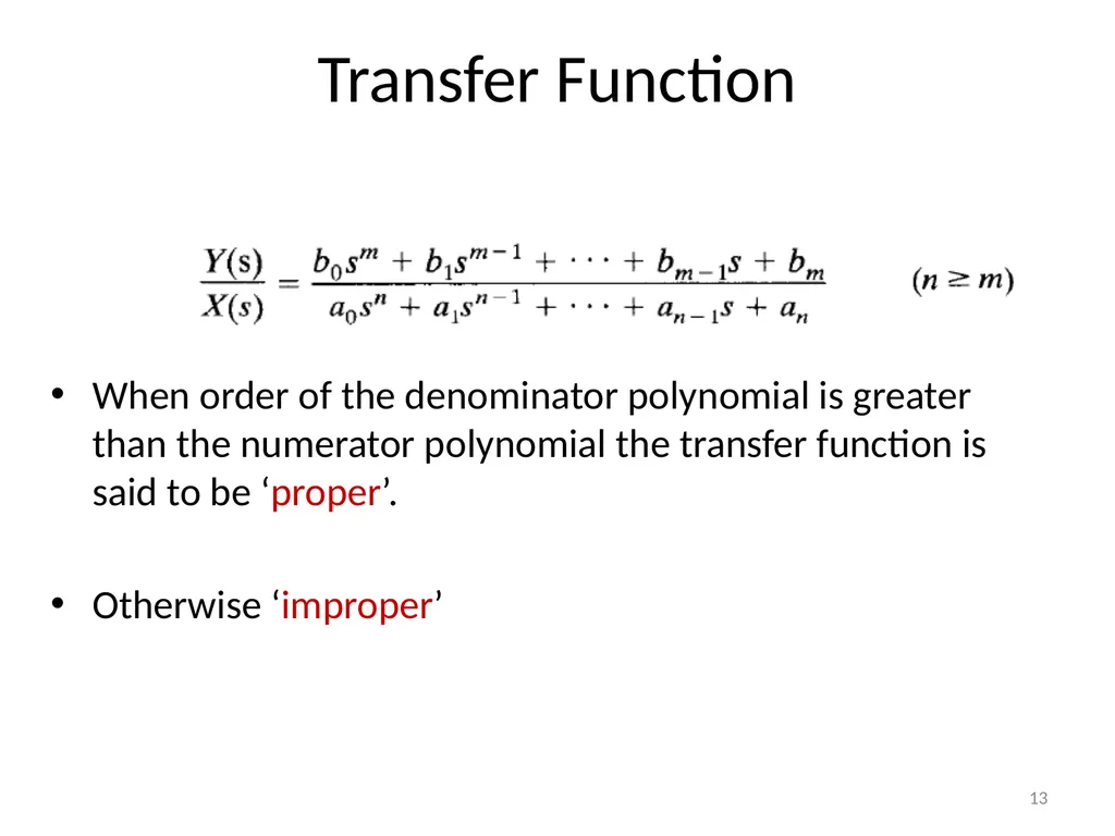
Transfer Function When order of the denominator polynomial is greater than the numerator polynomial the transfer function is said to be ‘proper’.
Otherwise ‘improper’ 13<br>
14
Transfer Function Transfer function helps us to check
The stability of the system
Time domain and frequency domain characteristics of the system
Response of the system for any given input 14<br>
15
Stability of Control System There are several meanings of stability, in general there are two kinds of stability definitions in control system study.
Absolute Stability
Relative Stability 15<br>
16
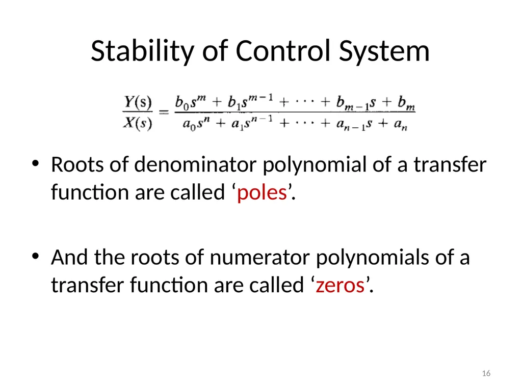
Stability of Control System Roots of denominator polynomial of a transfer function are called ‘poles’.
And the roots of numerator polynomials of a transfer function are called ‘zeros’. 16<br>
17
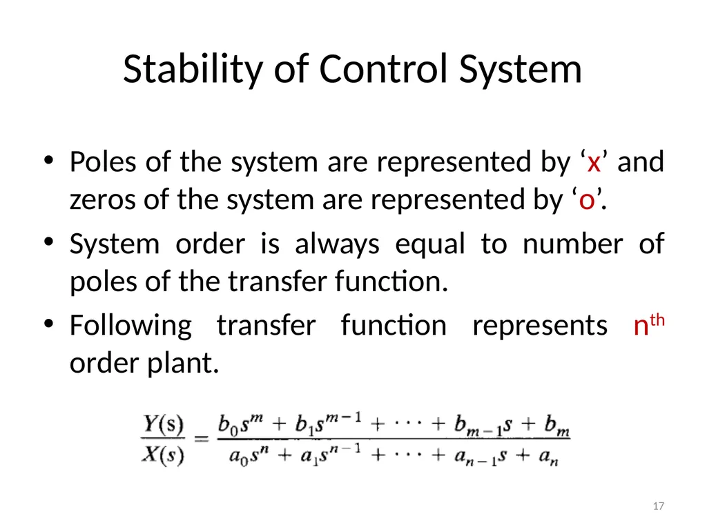
Stability of Control System Poles of the system are represented by ‘x’ and zeros of the system are represented by ‘o’.
System order is always equal to number of poles of the transfer function.
Following transfer function represents nth order plant. 17<br>
18
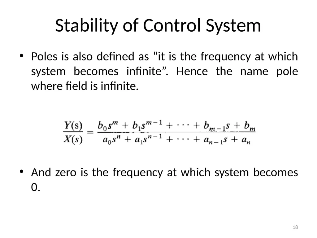
Stability of Control System Poles is also defined as “it is the frequency at which system becomes infinite”. Hence the name pole where field is infinite.
And zero is the frequency at which system becomes 0. 18<br>
19
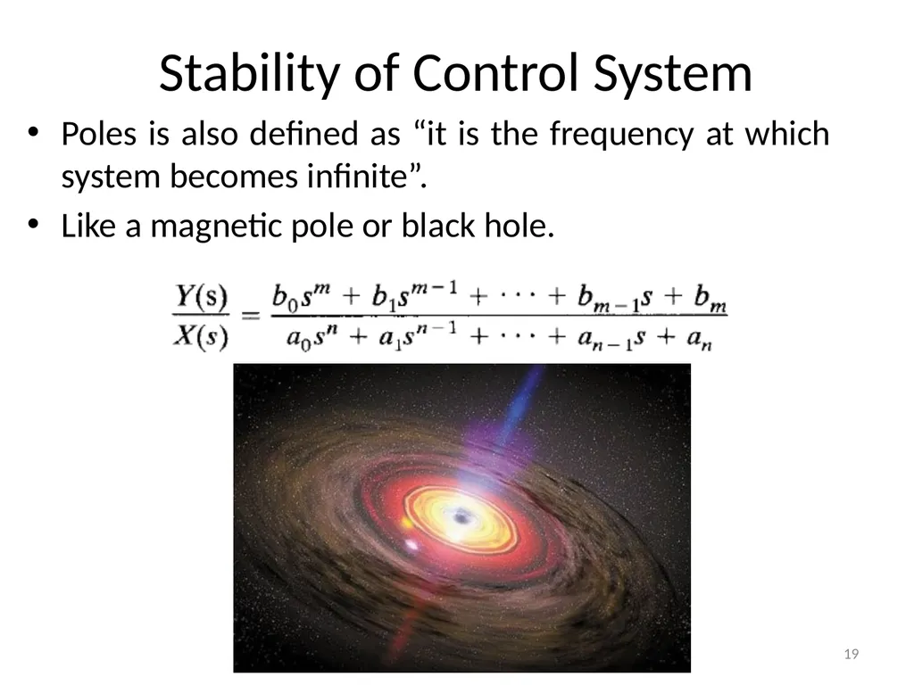
Stability of Control System Poles is also defined as “it is the frequency at which system becomes infinite”.
Like a magnetic pole or black hole. 19<br>
20
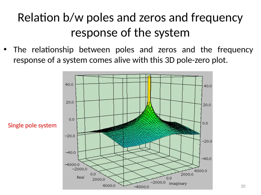
Relation b/w poles and zeros and frequency response of the system The relationship between poles and zeros and the frequency response of a system comes alive with this 3D pole-zero plot. 20 Single pole system<br>
21
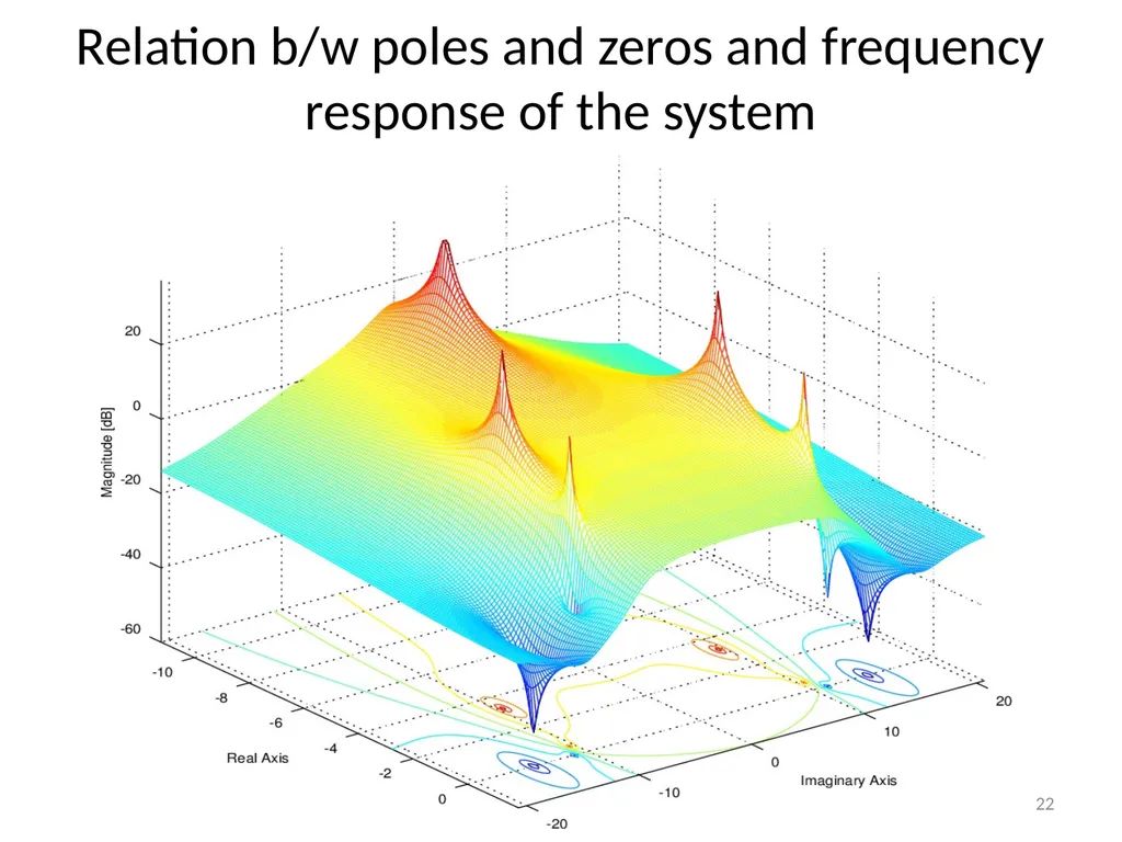
Relation b/w poles and zeros and frequency response of the system 3D pole-zero plot
System has 1 ‘zero’ and 2 ‘poles’. 21<br>
22
Relation b/w poles and zeros and frequency response of the system 22<br>
23
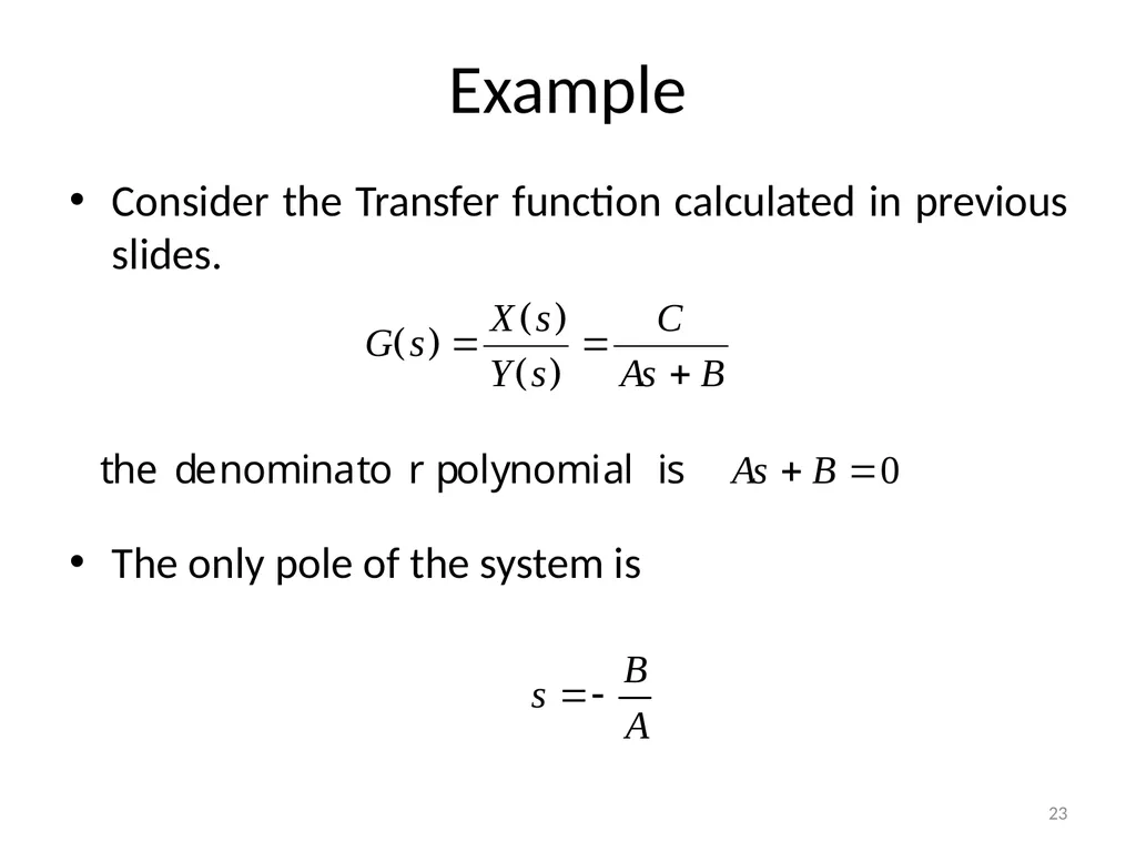
Example Consider the Transfer function calculated in previous slides.
The only pole of the system is 23<br>
24
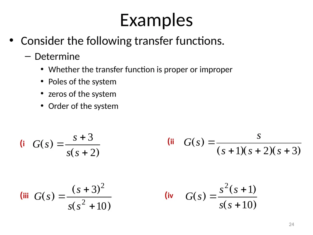
Examples Consider the following transfer functions.
Determine
Whether the transfer function is proper or improper
Poles of the system
zeros of the system
Order of the system 24 i) ii) iii) iv)<br>
25
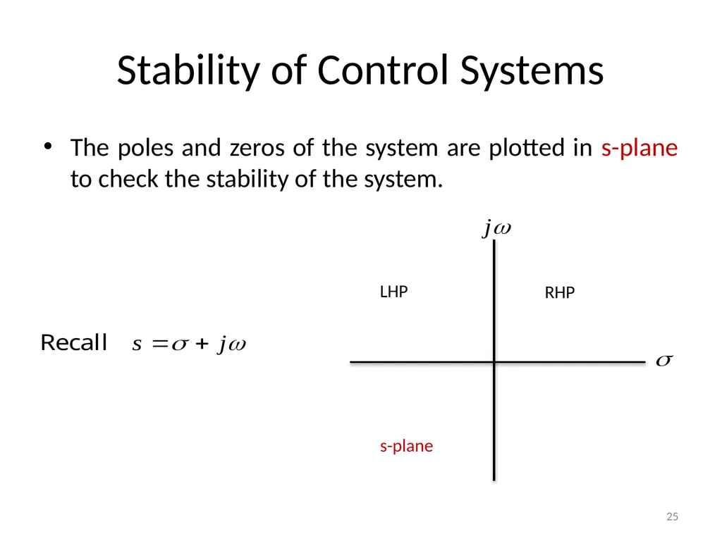
Stability of Control Systems The poles and zeros of the system are plotted in s-plane to check the stability of the system. 25<br>
26
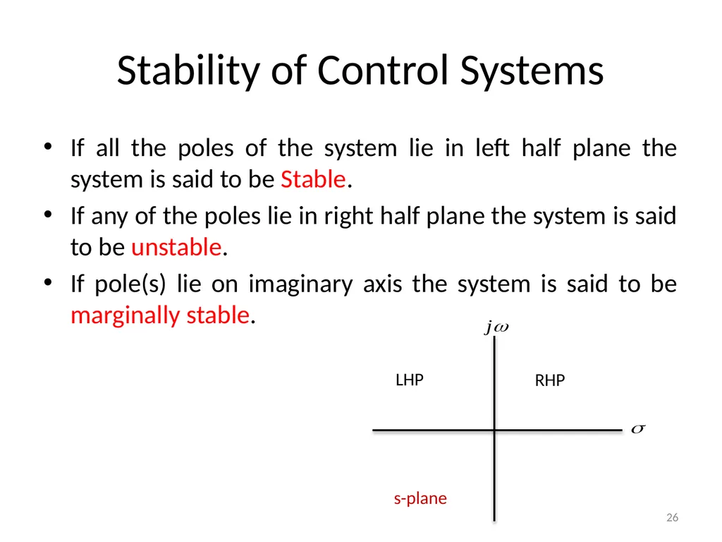
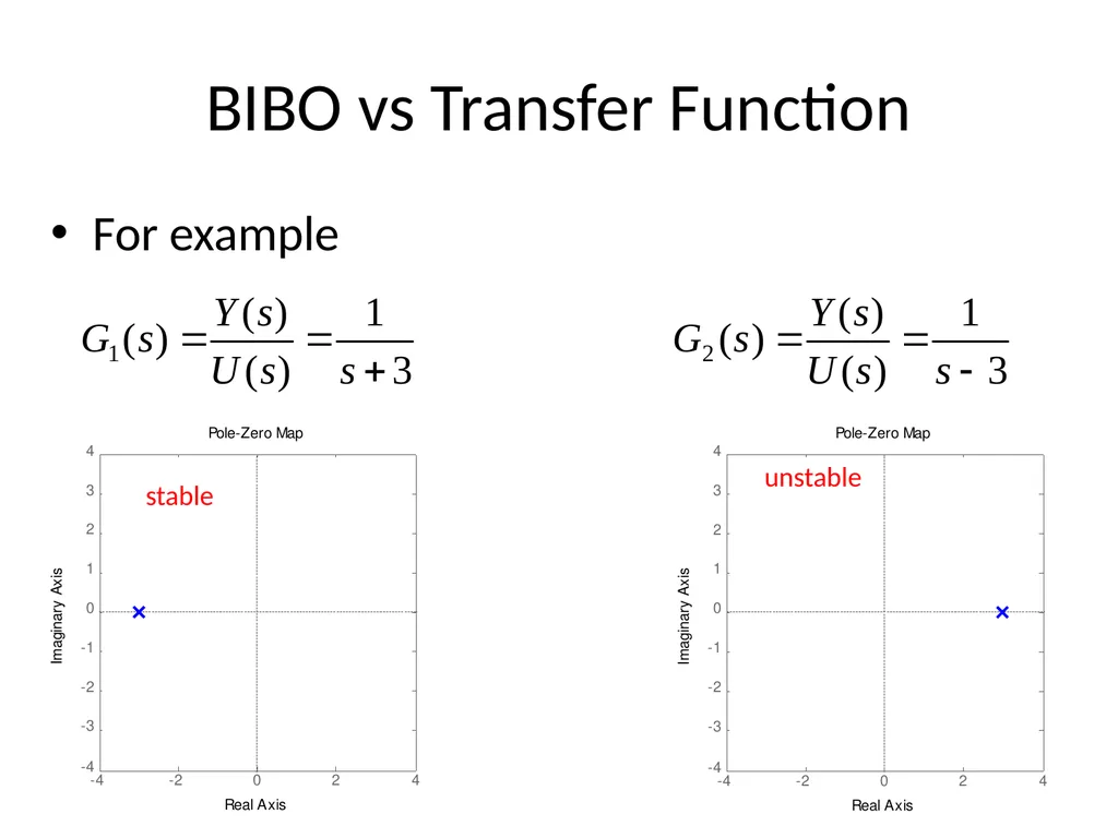
Stability of Control Systems If all the poles of the system lie in left half plane the system is said to be Stable.
If any of the poles lie in right half plane the system is said to be unstable.
If pole(s) lie on imaginary axis the system is said to be marginally stable. 26<br>
27
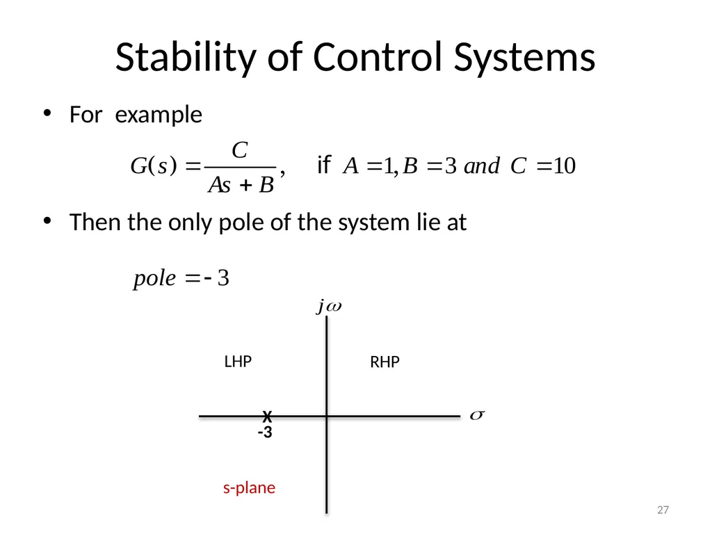
Stability of Control Systems For example
Then the only pole of the system lie at 27<br>
28
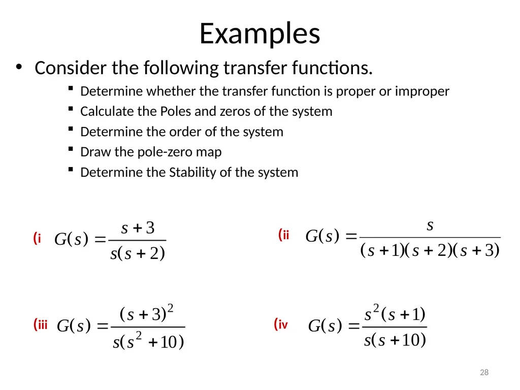
Examples Consider the following transfer functions.
Determine whether the transfer function is proper or improper
Calculate the Poles and zeros of the system
Determine the order of the system
Draw the pole-zero map
Determine the Stability of the system 28 i) ii) iii) iv)<br>
29
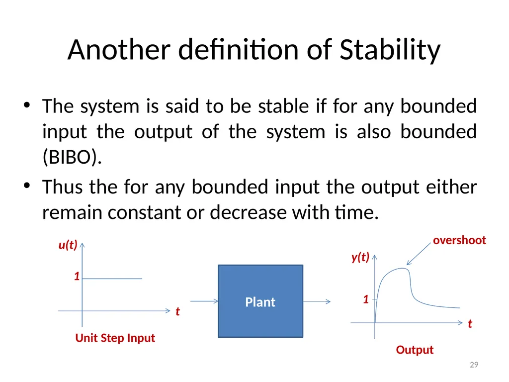
Another definition of Stability The system is said to be stable if for any bounded input the output of the system is also bounded (BIBO).
Thus the for any bounded input the output either remain constant or decrease with time. 29 1<br>
30
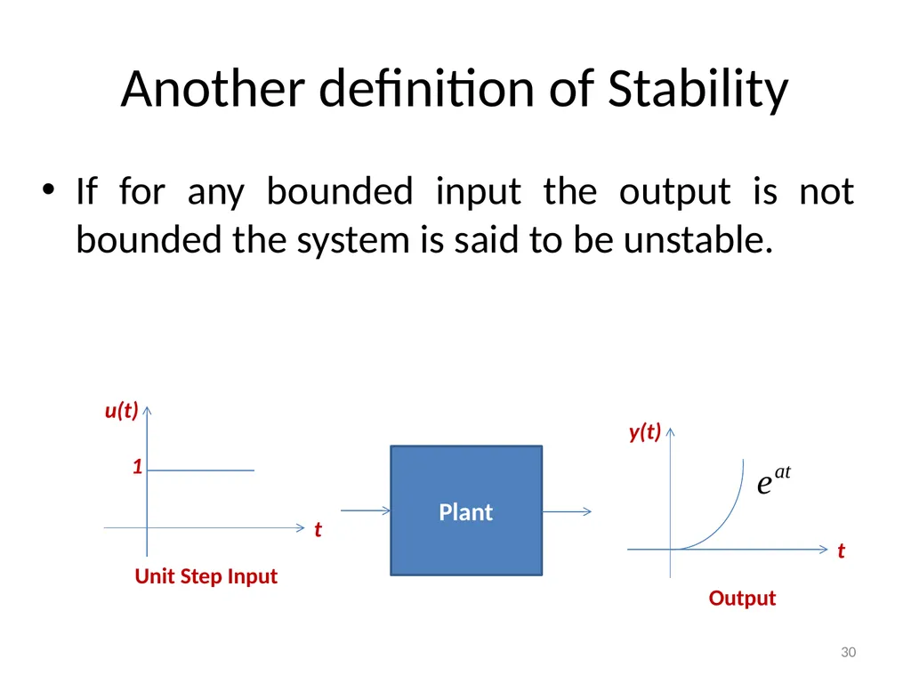
Another definition of Stability If for any bounded input the output is not bounded the system is said to be unstable. 30 Plant y(t) t Output<br>
31
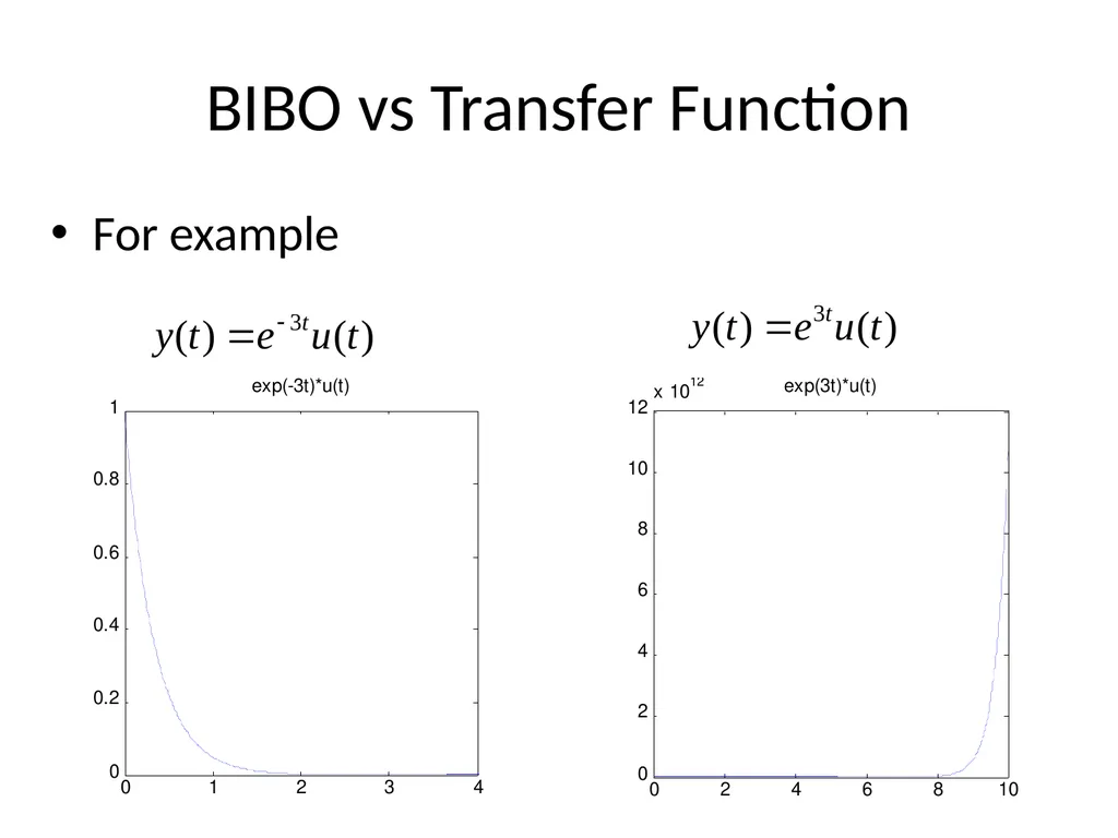
BIBO vs Transfer Function For example stable unstable<br>
32
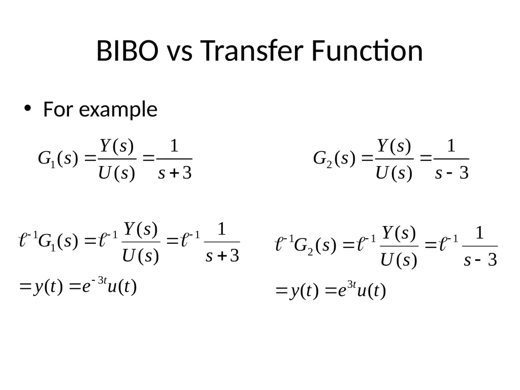
BIBO vs Transfer Function For example<br>
33
BIBO vs Transfer Function For example<br>
34
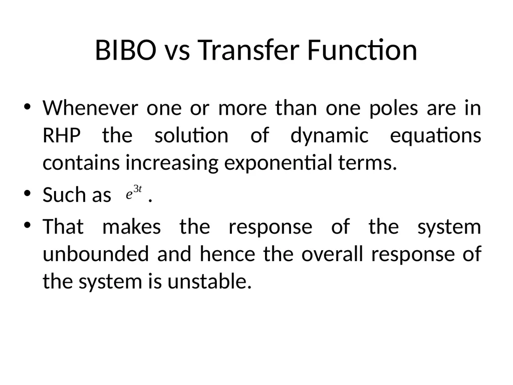
BIBO vs Transfer Function Whenever one or more than one poles are in RHP the solution of dynamic equations contains increasing exponential terms.
Such as .
That makes the response of the system unbounded and hence the overall response of the system is unstable.<br>
35
End of Lecture-2 To download this lecture visit
http://imtiazhussainkalwar.weebly.com/ 35<br>