
CPSC 422, Lecture 10 Slide 1 Intelligent Systems
Description: CPSC 422, Lecture 10 Slide 1 Intelligent Systems (AI-2) Computer Science cpsc422, Lecture 10 Sep, 30, 2015 CPSC 422, Lecture 10 2 Lecture Overview Finish Reinforcement learning Exploration vs. Exploitation On-policy Learning (SARSA)
Related Topics
Download Presentation
"CPSC 422, Lecture 10 Slide 1 Intelligent Systems" is the property of its rightful owner. Permission is granted to download and print the materials on this website for personal, non-commercial use only, and to display it on your personal computer provided you do not modify the materials and that you retain all copyright notices contained in the materials. By downloading content from our website, you accept the terms of this agreement.
Presentation Transcript
slide1. CPSC 422, Lecture 10 Slide 1 Intelligent Systems (AI-2)
Computer Science cpsc422, Lecture 10
Sep, 30, 2015<br>
slide2. CPSC 422, Lecture 10 2 Lecture Overview Finish Reinforcement learning
Exploration vs. Exploitation
On-policy Learning (SARSA)
Scalability<br>
slide3. CPSC 422, Lecture 10 Slide 3<br>
slide4. Clarification on the ak CPSC 422, Lecture 10 4<br>
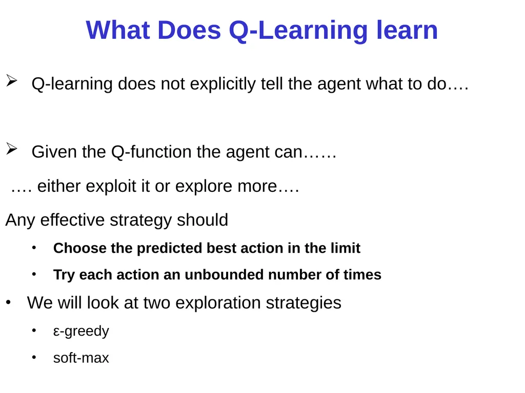
slide5. What Does Q-Learning learn Q-learning does not explicitly tell the agent what to do….
Given the Q-function the agent can……
…. either exploit it or explore more….
Any effective strategy should
Choose the predicted best action in the limit
Try each action an unbounded number of times
We will look at two exploration strategies
ε-greedy
soft-max CPSC 422, Lecture 10 5<br>
slide6. Exploration Strategies Hard to come up with an optimal exploration policy (problem is widely studied in statistical decision theory)
But intuitively, any such strategy should be greedy in the limit of infinite exploration (GLIE), i.e.
Choose the predicted best action in the limit
Try each action an unbounded number of times
We will look at two exploration strategies
ε-greedy
soft-max CPSC 422, Lecture 8 6<br>
slide7. ε-greedy Choose a random action with probability ε and choose a best action with probability 1- ε
Eventually converges to an optimal policy because it ensures that the first GLIE condition (try every action an unbounded number of times) is satisfied via the ε random selection
But it is rather slow
It always chooses the non-optimal action with probability ε, while ideally you would want to…….
Fix: vary ε overtime CPSC 422, Lecture 10 7<br>
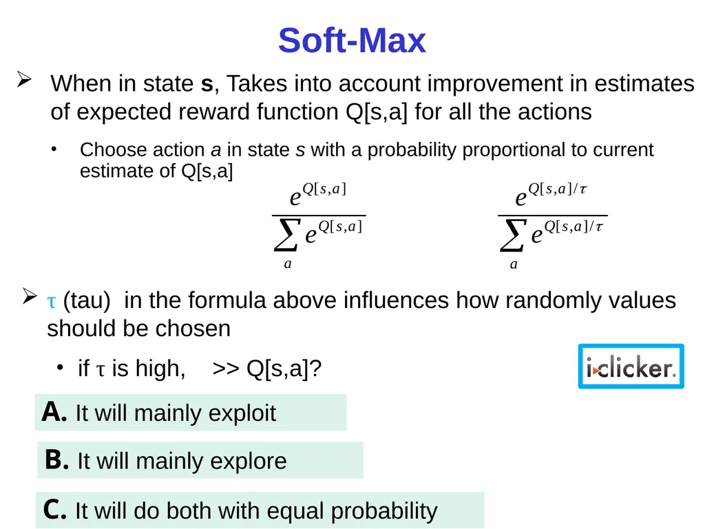
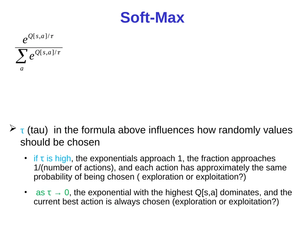
slide8. Soft-Max When in state s, Takes into account improvement in estimates of expected reward function Q[s,a] for all the actions
Choose action a in state s with a probability proportional to current estimate of Q[s,a] τ (tau) in the formula above influences how randomly values should be chosen
if τ is high, >> Q[s,a]? CPSC 422, Lecture 10 8 A. It will mainly exploit B. It will mainly explore C. It will do both with equal probability<br>
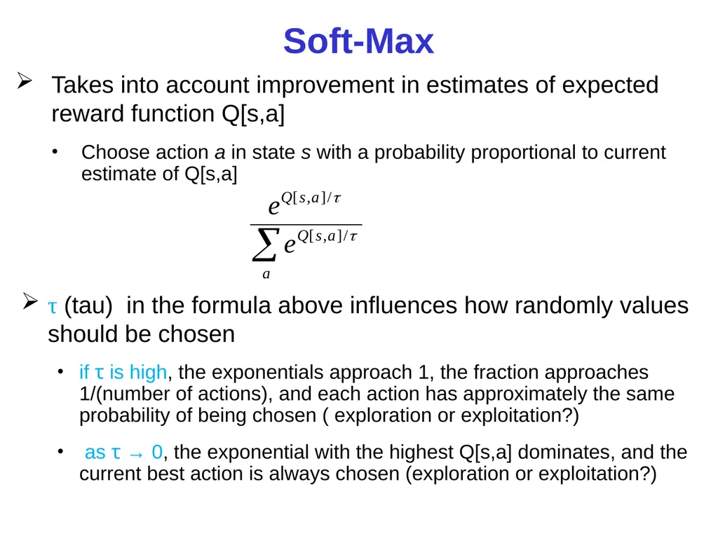
slide9. Soft-Max Takes into account improvement in estimates of expected reward function Q[s,a]
Choose action a in state s with a probability proportional to current estimate of Q[s,a] τ (tau) in the formula above influences how randomly values should be chosen
if τ is high, the exponentials approach 1, the fraction approaches 1/(number of actions), and each action has approximately the same probability of being chosen ( exploration or exploitation?)
as τ → 0, the exponential with the highest Q[s,a] dominates, and the current best action is always chosen (exploration or exploitation?) CPSC 422, Lecture 10 9<br>
slide10. Soft-Max τ (tau) in the formula above influences how randomly values should be chosen
if τ is high, the exponentials approach 1, the fraction approaches 1/(number of actions), and each action has approximately the same probability of being chosen ( exploration or exploitation?)
as τ → 0, the exponential with the highest Q[s,a] dominates, and the current best action is always chosen (exploration or exploitation?) CPSC 422, Lecture 10 10<br>
slide11. CPSC 422, Lecture 10 11 Lecture Overview Finish Reinforcement learning
Exploration vs. Exploitation
On-policy Learning (SARSA)
RL scalability<br>
slide12. Learning before vs. during deployment Our learning agent can:
act in the environment to learn how it works: first learn an optimal policy, then use this policy to act (there is a learning phase before deployment)
Learn as you go: start operating in the environment right away and learn from actions (learning happens during deployment)
If there is time to learn before deployment, the agent should try to do its best to learn as much as possible about the environment
even engage in locally suboptimal behaviors, because this will guarantee reaching an optimal policy in the long run
If learning while “at work”, suboptimal behaviors could be costly CPSC 422, Lecture 10 12<br>
slide13. Learning before vs. during deployment Our learning agent can:
act in the environment to learn how it works (before deployment)
Learn as you go (after deployment)
If there is time to learn before deployment, the agent should try to do its best to learn as much as possible about the environment
even engage in locally suboptimal behaviors, because this will guarantee reaching an optimal policy in the long run
If learning while “at work”, suboptimal behaviors could be costly CPSC 422, Lecture 10 13<br>
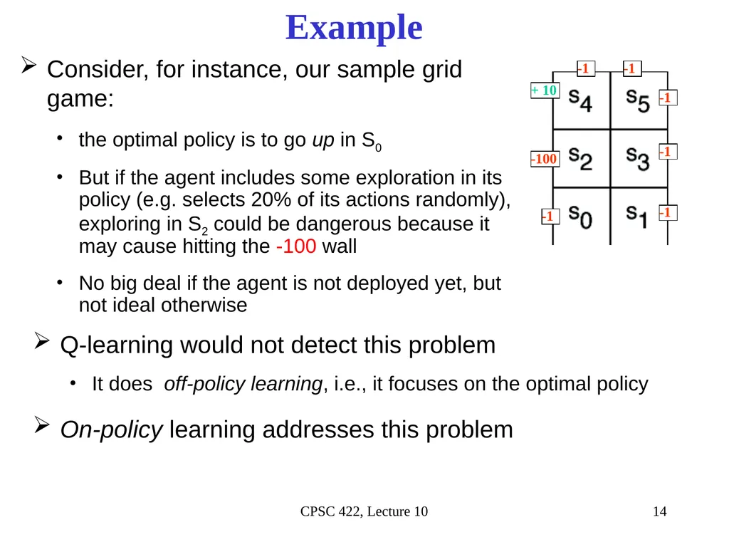
slide14. Example Consider, for instance, our sample grid game:
the optimal policy is to go up in S0
But if the agent includes some exploration in its policy (e.g. selects 20% of its actions randomly), exploring in S2 could be dangerous because it may cause hitting the -100 wall
No big deal if the agent is not deployed yet, but not ideal otherwise Q-learning would not detect this problem
It does off-policy learning, i.e., it focuses on the optimal policy
On-policy learning addresses this problem CPSC 422, Lecture 10 14<br>
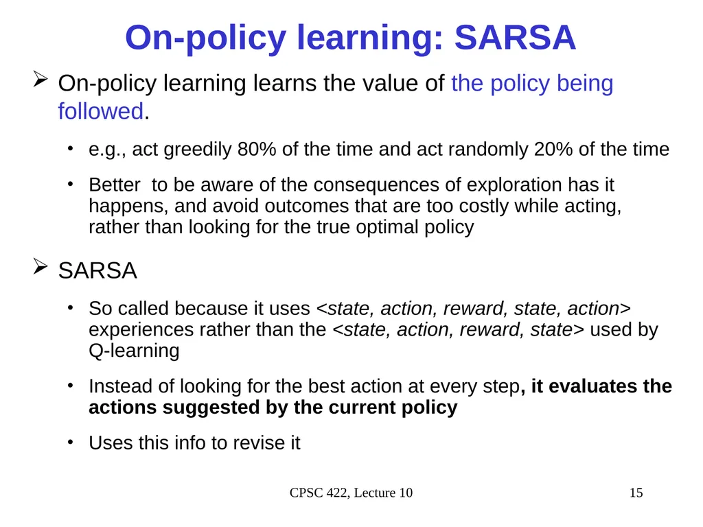
slide15. On-policy learning: SARSA On-policy learning learns the value of the policy being followed.
e.g., act greedily 80% of the time and act randomly 20% of the time
Better to be aware of the consequences of exploration has it happens, and avoid outcomes that are too costly while acting, rather than looking for the true optimal policy
SARSA
So called because it uses <state, action, reward, state, action> experiences rather than the <state, action, reward, state> used by Q-learning
Instead of looking for the best action at every step, it evaluates the actions suggested by the current policy
Uses this info to revise it CPSC 422, Lecture 10 15<br>
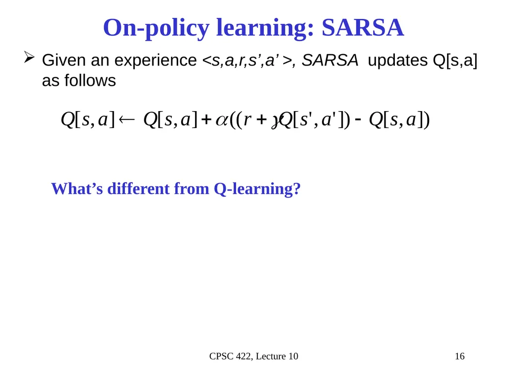
slide16. On-policy learning: SARSA Given an experience <s,a,r,s’,a’ >, SARSA updates Q[s,a] as follows What’s different from Q-learning? CPSC 422, Lecture 10 16<br>
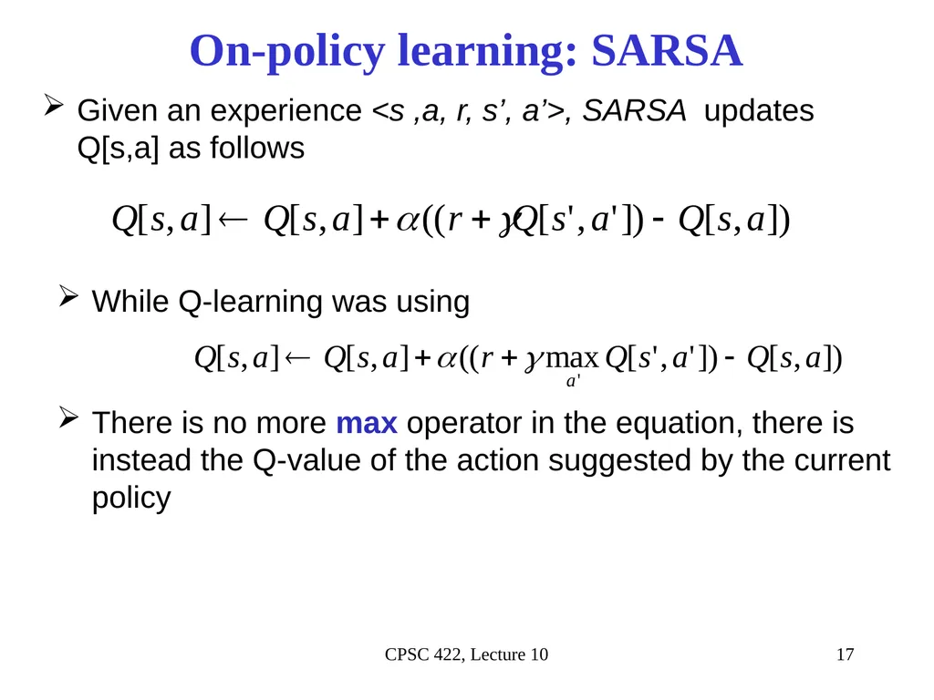
slide17. On-policy learning: SARSA Given an experience <s ,a, r, s’, a’>, SARSA updates Q[s,a] as follows While Q-learning was using
There is no more max operator in the equation, there is instead the Q-value of the action suggested by the current policy CPSC 422, Lecture 10 17<br>
slide18. On-policy learning: SARSA Does SARSA remind you of any other algorithm we have seen before? (not for 422) CPSC 422, Lecture 10 18<br>
slide19. Policy Iteration Algorithm
π ← an arbitrary initial policy, U ← A vector of utility values, initially 0
2. Repeat until no change in π
Compute new utilities given π and current U (policy evaluation)
(b) Update π as if utilities were correct (policy improvement) Expected value of following current пi from s Expected value of following another action in s Policy
Improvement
step CPSC 422, Lecture 10 19<br>
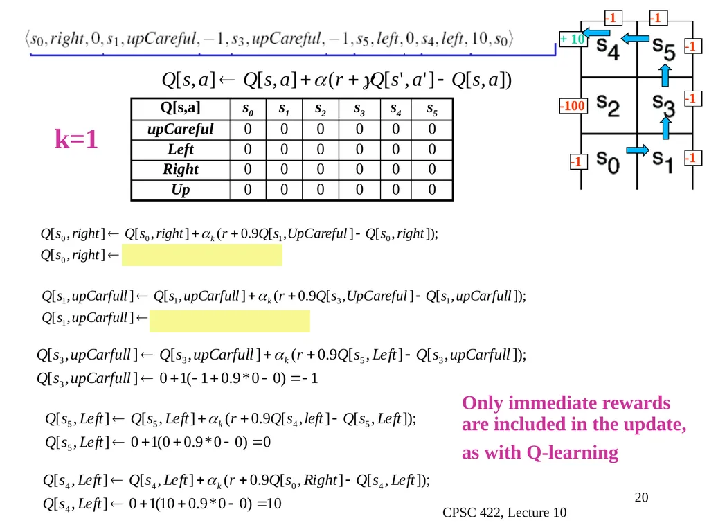
slide20. k=1 k=1 Only immediate rewards
are included in the update,
as with Q-learning CPSC 422, Lecture 10 20<br>
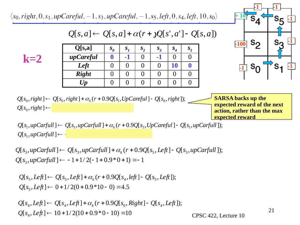
slide21. k=1 k=2 SARSA backs up the expected reward of the next action, rather than the max expected reward CPSC 422, Lecture 10 21<br>
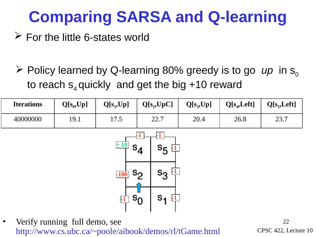
slide22. Comparing SARSA and Q-learning For the little 6-states world Policy learned by Q-learning 80% greedy is to go up in s0 to reach s4 quickly and get the big +10 reward CPSC 422, Lecture 10 22 Verify running full demo, see http://www.cs.ubc.ca/~poole/aibook/demos/rl/tGame.html<br>
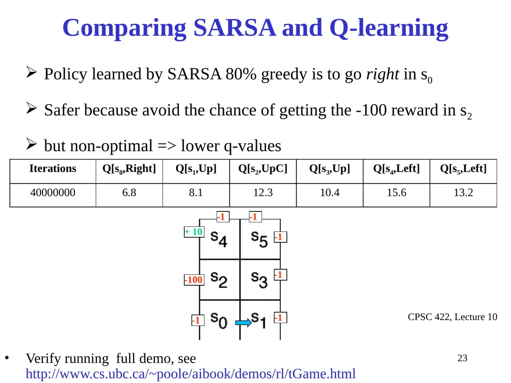
slide23. Comparing SARSA and Q-learning Policy learned by SARSA 80% greedy is to go right in s0
Safer because avoid the chance of getting the -100 reward in s2
but non-optimal => lower q-values CPSC 422, Lecture 10 23 Verify running full demo, see http://www.cs.ubc.ca/~poole/aibook/demos/rl/tGame.html<br>
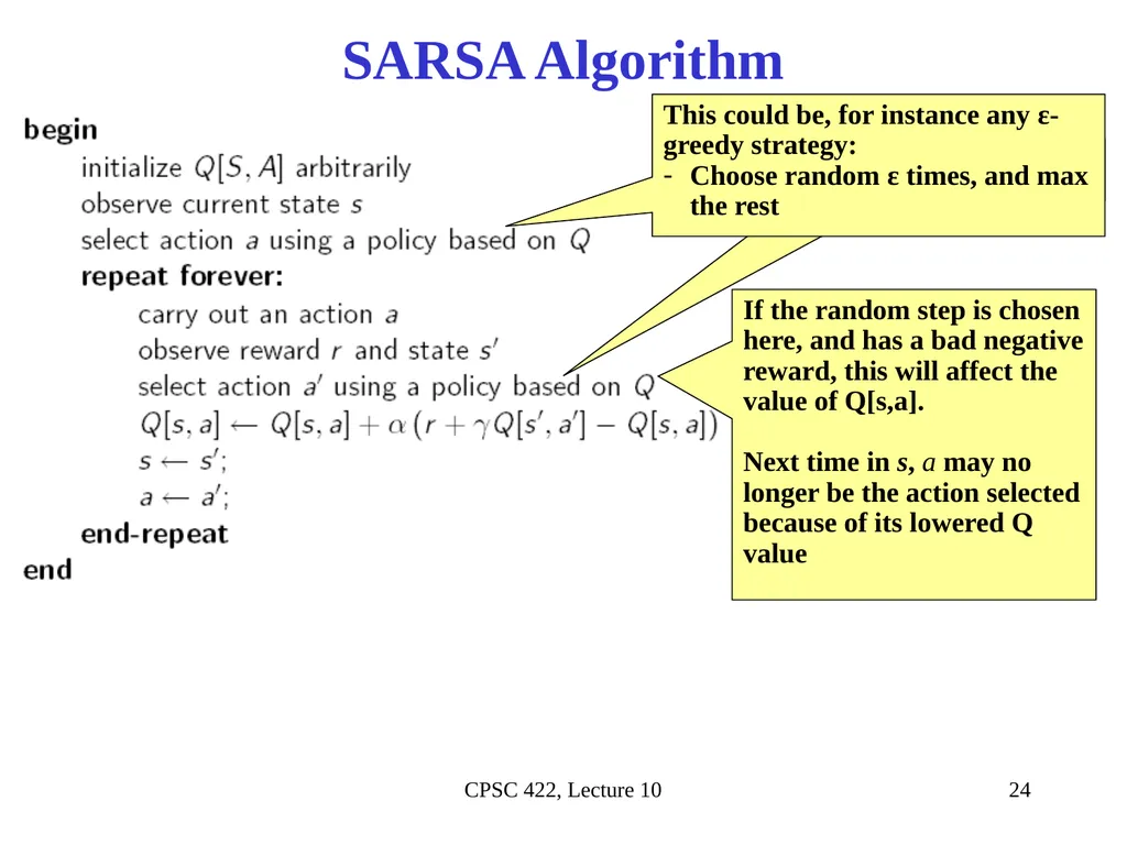
slide24. SARSA Algorithm This could be, for instance any ε-greedy strategy:
- Choose random ε times, and max the rest This could be, for instance any ε-greedy strategy:
Choose random ε times, and max the rest If the random step is chosen here, and has a bad negative reward, this will affect the value of Q[s,a].
Next time in s, a may no longer be the action selected because of its lowered Q value CPSC 422, Lecture 10 24<br>
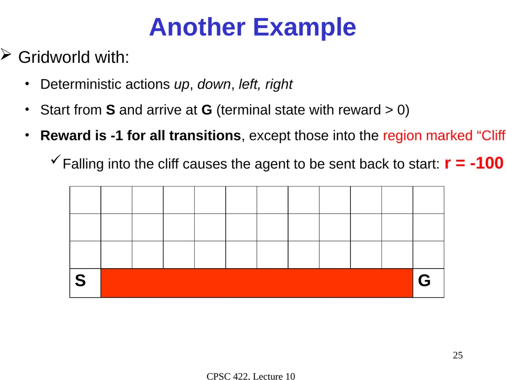
slide25. Another Example Gridworld with:
Deterministic actions up, down, left, right
Start from S and arrive at G (terminal state with reward > 0)
Reward is -1 for all transitions, except those into the region marked “Cliff”
Falling into the cliff causes the agent to be sent back to start: r = -100 CPSC 422, Lecture 10 25<br>
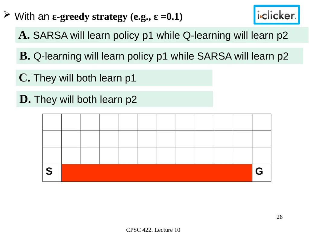
slide26. With an ε-greedy strategy (e.g., ε =0.1) CPSC 422, Lecture 10 26 A. SARSA will learn policy p1 while Q-learning will learn p2 B. Q-learning will learn policy p1 while SARSA will learn p2 C. They will both learn p1 D. They will both learn p2<br>
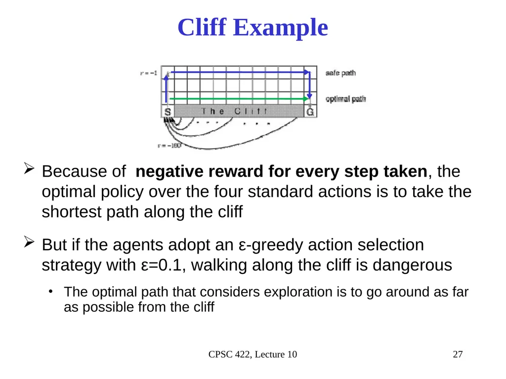
slide27. Cliff Example Because of negative reward for every step taken, the optimal policy over the four standard actions is to take the shortest path along the cliff
But if the agents adopt an ε-greedy action selection strategy with ε=0.1, walking along the cliff is dangerous
The optimal path that considers exploration is to go around as far as possible from the cliff CPSC 422, Lecture 10 27<br>
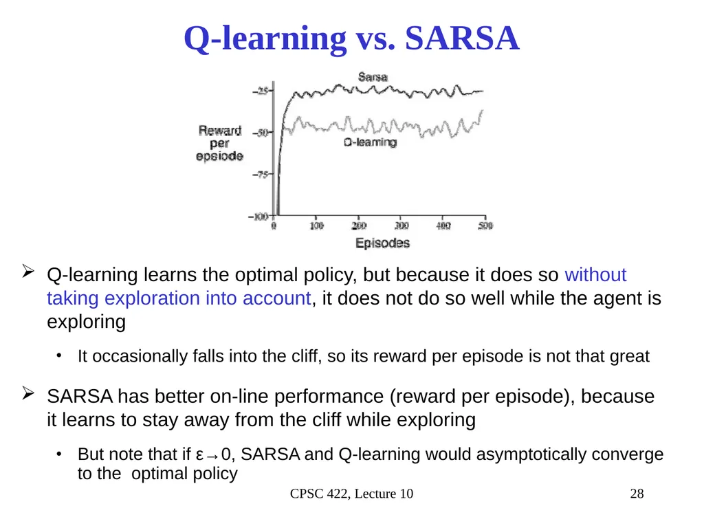
slide28. Q-learning vs. SARSA Q-learning learns the optimal policy, but because it does so without taking exploration into account, it does not do so well while the agent is exploring
It occasionally falls into the cliff, so its reward per episode is not that great
SARSA has better on-line performance (reward per episode), because it learns to stay away from the cliff while exploring
But note that if ε→0, SARSA and Q-learning would asymptotically converge to the optimal policy CPSC 422, Lecture 10 28<br>
slide29. RL scalability: Policy Gradient Methods (not for 422) Problems for most value-function methods (like Q-L, SARSA)
Continuous states and actions in high dimensional spaces
Uncertainty on the state information
Convergence CPSC 422, Lecture 10 29 Popular Solution: Policy Gradient Methods…. But still limited
On-policy by definition (like SARSA)
Find Local maximum (while global for value-function methods)
Open Parameter: learning rate (to be set empirically)<br>
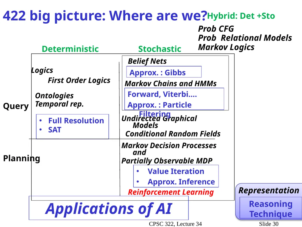
slide30. 422 big picture: Where are we? CPSC 322, Lecture 34 Slide 30<br>
slide31. CPSC 422, Lecture 10 Slide 31 Learning Goals for today’s class You can:
Describe and compare techniques to combine exploration with exploitation
On-policy Learning (SARSA)
Discuss trade-offs in RL scalability (not required)<br>
slide32. CPSC 422, Lecture 10 Slide 32 TODO for Fri Read textbook 6.4.2
Next research paper will be next Wed
Practice Ex 11.B<br>
slide33. Problem with Model-free methods Q-learning and SARSA are model-free methods
What does this mean? CPSC 422, Lecture 10 33<br>
slide34. Problems With Model-free Methods Q-learning and SARSA are model-free methods
They do not need to learn the transition and/or reward model, they are implicitly taken into account via experiences
Sounds handy, but there is a main disadvantage:
How often does the agent get to update its Q-estimates? CPSC 422, Lecture 10 34<br>
slide35. Problems with Model-free Methods Q-learning and SARSA are model-free methods
They do not need to learn the transition and/or reward model, they are implicitly taken into account via experiences
Sounds handy, but there is a main disadvantage:
How often does the agent get to update its Q-estimates?
Only after a new experience comes in
Great if the agent acts very frequently, not so great if actions are sparse, because it wastes computation time CPSC 422, Lecture 10 35<br>
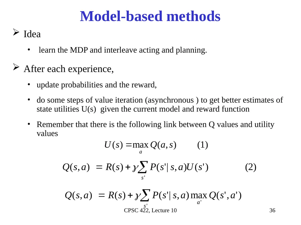
slide36. Model-based methods Idea
learn the MDP and interleave acting and planning.
After each experience,
update probabilities and the reward,
do some steps of value iteration (asynchronous ) to get better estimates of state utilities U(s) given the current model and reward function
Remember that there is the following link between Q values and utility values CPSC 422, Lecture 10 36<br>
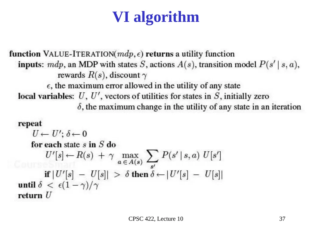
slide37. VI algorithm CPSC 422, Lecture 10 37<br>
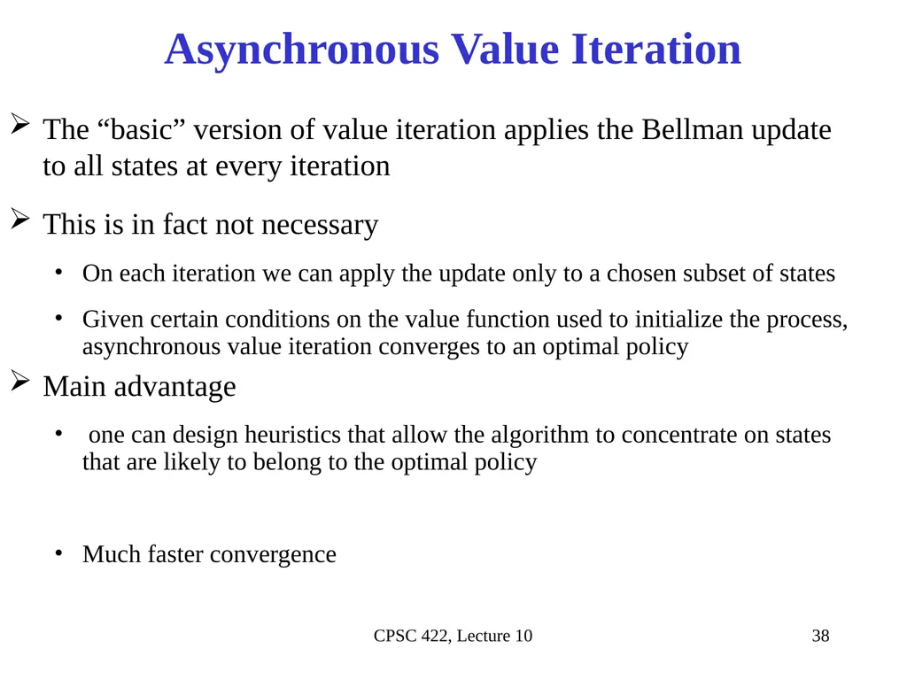
slide38. Asynchronous Value Iteration The “basic” version of value iteration applies the Bellman update to all states at every iteration
This is in fact not necessary
On each iteration we can apply the update only to a chosen subset of states
Given certain conditions on the value function used to initialize the process, asynchronous value iteration converges to an optimal policy Main advantage
one can design heuristics that allow the algorithm to concentrate on states that are likely to belong to the optimal policy
Much faster convergence CPSC 422, Lecture 10 38<br>
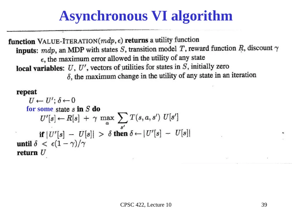
slide39. Asynchronous VI algorithm for some CPSC 422, Lecture 10 39<br>
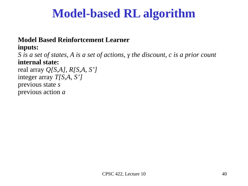
slide40. Model-based RL algorithm Model Based Reinfortcement Learner
inputs:
S is a set of states, A is a set of actions, γ the discount, c is a prior count
internal state:
real array Q[S,A], R[S,A, S’]
integer array T[S,A, S’]
previous state s
previous action a CPSC 422, Lecture 10 40<br>
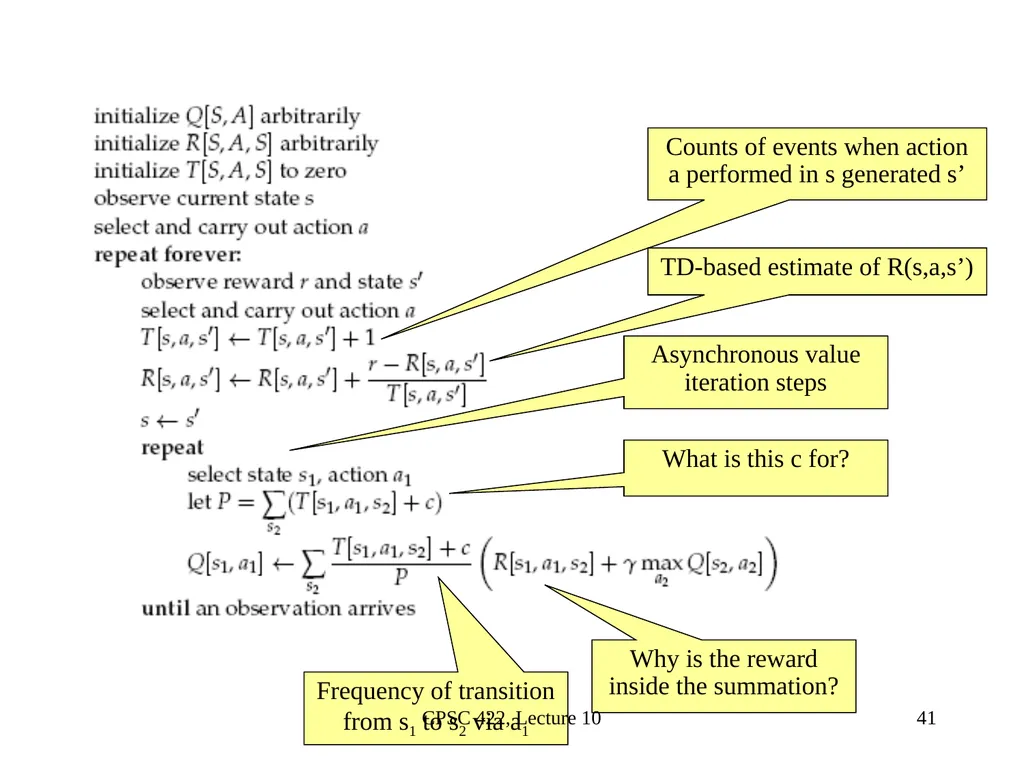
slide41. Counts of events when action a performed in s generated s’ TD-based estimate of R(s,a,s’) Asynchronous value iteration steps Frequency of transition from s1 to s2 via a1 Why is the reward inside the summation? What is this c for? CPSC 422, Lecture 10 41<br>
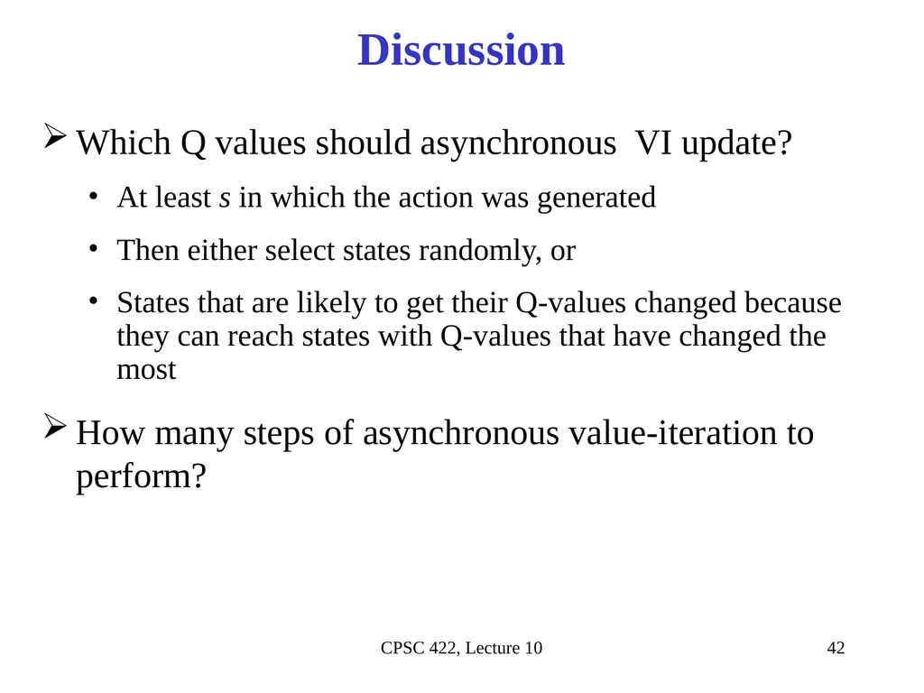
slide42. Discussion Which Q values should asynchronous VI update?
At least s in which the action was generated
Then either select states randomly, or
States that are likely to get their Q-values changed because they can reach states with Q-values that have changed the most
How many steps of asynchronous value-iteration to perform? CPSC 422, Lecture 10 42<br>
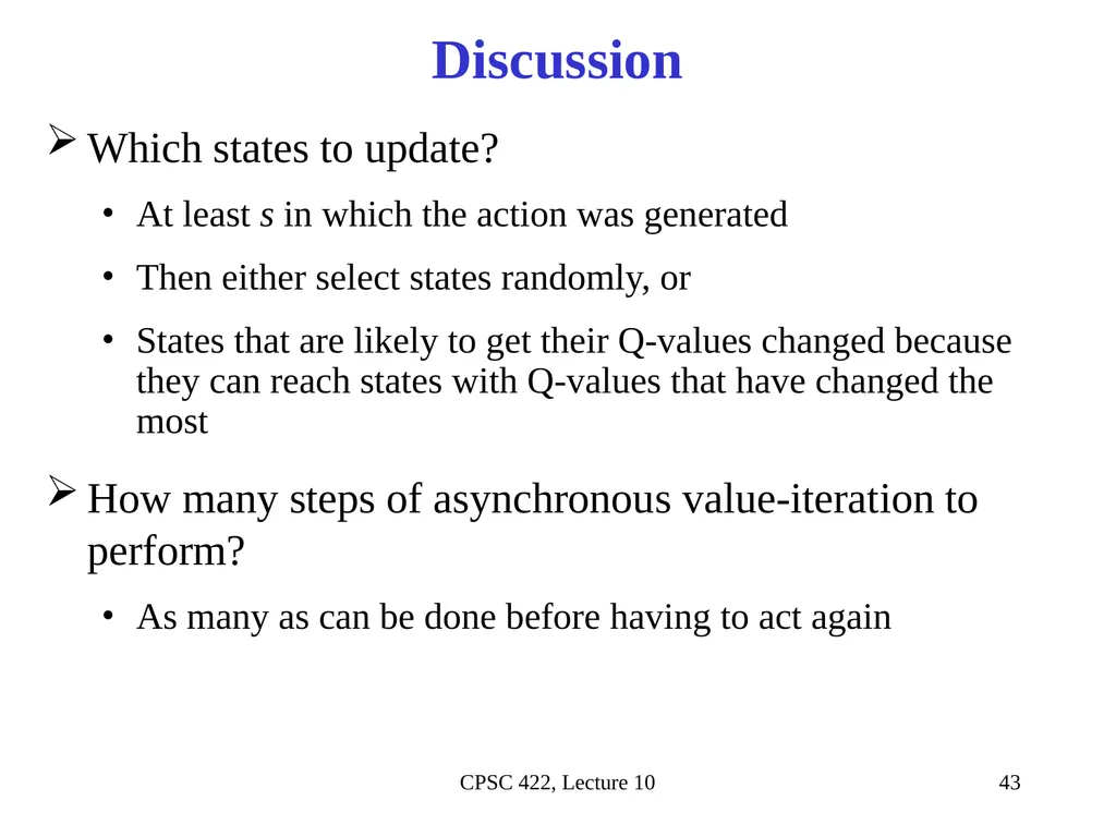
slide43. Discussion Which states to update?
At least s in which the action was generated
Then either select states randomly, or
States that are likely to get their Q-values changed because they can reach states with Q-values that have changed the most
How many steps of asynchronous value-iteration to perform?
As many as can be done before having to act again CPSC 422, Lecture 10 43<br>
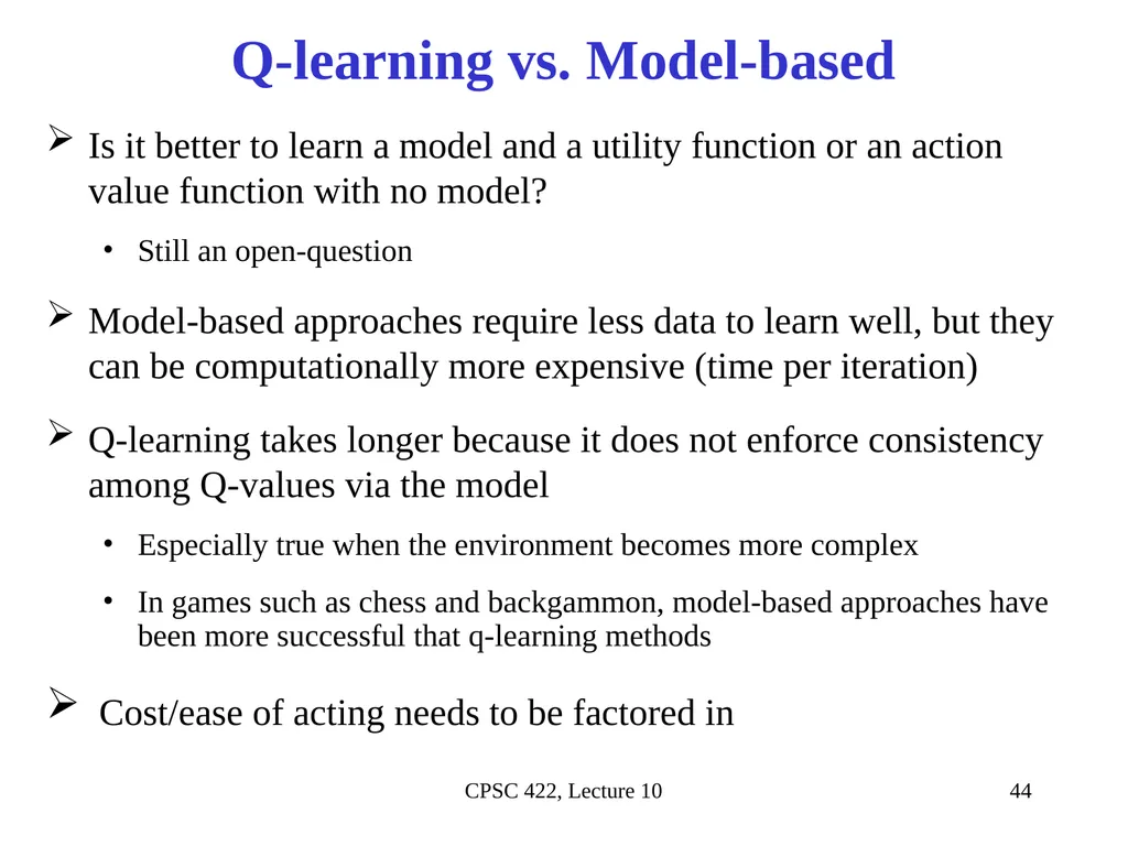
slide44. Q-learning vs. Model-based Is it better to learn a model and a utility function or an action value function with no model?
Still an open-question
Model-based approaches require less data to learn well, but they can be computationally more expensive (time per iteration)
Q-learning takes longer because it does not enforce consistency among Q-values via the model
Especially true when the environment becomes more complex
In games such as chess and backgammon, model-based approaches have been more successful that q-learning methods
Cost/ease of acting needs to be factored in CPSC 422, Lecture 10 44<br>
Computer Science cpsc422, Lecture 10
Sep, 30, 2015<br>
slide2. CPSC 422, Lecture 10 2 Lecture Overview Finish Reinforcement learning
Exploration vs. Exploitation
On-policy Learning (SARSA)
Scalability<br>
slide3. CPSC 422, Lecture 10 Slide 3<br>
slide4. Clarification on the ak CPSC 422, Lecture 10 4<br>
slide5. What Does Q-Learning learn Q-learning does not explicitly tell the agent what to do….
Given the Q-function the agent can……
…. either exploit it or explore more….
Any effective strategy should
Choose the predicted best action in the limit
Try each action an unbounded number of times
We will look at two exploration strategies
ε-greedy
soft-max CPSC 422, Lecture 10 5<br>
slide6. Exploration Strategies Hard to come up with an optimal exploration policy (problem is widely studied in statistical decision theory)
But intuitively, any such strategy should be greedy in the limit of infinite exploration (GLIE), i.e.
Choose the predicted best action in the limit
Try each action an unbounded number of times
We will look at two exploration strategies
ε-greedy
soft-max CPSC 422, Lecture 8 6<br>
slide7. ε-greedy Choose a random action with probability ε and choose a best action with probability 1- ε
Eventually converges to an optimal policy because it ensures that the first GLIE condition (try every action an unbounded number of times) is satisfied via the ε random selection
But it is rather slow
It always chooses the non-optimal action with probability ε, while ideally you would want to…….
Fix: vary ε overtime CPSC 422, Lecture 10 7<br>
slide8. Soft-Max When in state s, Takes into account improvement in estimates of expected reward function Q[s,a] for all the actions
Choose action a in state s with a probability proportional to current estimate of Q[s,a] τ (tau) in the formula above influences how randomly values should be chosen
if τ is high, >> Q[s,a]? CPSC 422, Lecture 10 8 A. It will mainly exploit B. It will mainly explore C. It will do both with equal probability<br>
slide9. Soft-Max Takes into account improvement in estimates of expected reward function Q[s,a]
Choose action a in state s with a probability proportional to current estimate of Q[s,a] τ (tau) in the formula above influences how randomly values should be chosen
if τ is high, the exponentials approach 1, the fraction approaches 1/(number of actions), and each action has approximately the same probability of being chosen ( exploration or exploitation?)
as τ → 0, the exponential with the highest Q[s,a] dominates, and the current best action is always chosen (exploration or exploitation?) CPSC 422, Lecture 10 9<br>
slide10. Soft-Max τ (tau) in the formula above influences how randomly values should be chosen
if τ is high, the exponentials approach 1, the fraction approaches 1/(number of actions), and each action has approximately the same probability of being chosen ( exploration or exploitation?)
as τ → 0, the exponential with the highest Q[s,a] dominates, and the current best action is always chosen (exploration or exploitation?) CPSC 422, Lecture 10 10<br>
slide11. CPSC 422, Lecture 10 11 Lecture Overview Finish Reinforcement learning
Exploration vs. Exploitation
On-policy Learning (SARSA)
RL scalability<br>
slide12. Learning before vs. during deployment Our learning agent can:
act in the environment to learn how it works: first learn an optimal policy, then use this policy to act (there is a learning phase before deployment)
Learn as you go: start operating in the environment right away and learn from actions (learning happens during deployment)
If there is time to learn before deployment, the agent should try to do its best to learn as much as possible about the environment
even engage in locally suboptimal behaviors, because this will guarantee reaching an optimal policy in the long run
If learning while “at work”, suboptimal behaviors could be costly CPSC 422, Lecture 10 12<br>
slide13. Learning before vs. during deployment Our learning agent can:
act in the environment to learn how it works (before deployment)
Learn as you go (after deployment)
If there is time to learn before deployment, the agent should try to do its best to learn as much as possible about the environment
even engage in locally suboptimal behaviors, because this will guarantee reaching an optimal policy in the long run
If learning while “at work”, suboptimal behaviors could be costly CPSC 422, Lecture 10 13<br>
slide14. Example Consider, for instance, our sample grid game:
the optimal policy is to go up in S0
But if the agent includes some exploration in its policy (e.g. selects 20% of its actions randomly), exploring in S2 could be dangerous because it may cause hitting the -100 wall
No big deal if the agent is not deployed yet, but not ideal otherwise Q-learning would not detect this problem
It does off-policy learning, i.e., it focuses on the optimal policy
On-policy learning addresses this problem CPSC 422, Lecture 10 14<br>
slide15. On-policy learning: SARSA On-policy learning learns the value of the policy being followed.
e.g., act greedily 80% of the time and act randomly 20% of the time
Better to be aware of the consequences of exploration has it happens, and avoid outcomes that are too costly while acting, rather than looking for the true optimal policy
SARSA
So called because it uses <state, action, reward, state, action> experiences rather than the <state, action, reward, state> used by Q-learning
Instead of looking for the best action at every step, it evaluates the actions suggested by the current policy
Uses this info to revise it CPSC 422, Lecture 10 15<br>
slide16. On-policy learning: SARSA Given an experience <s,a,r,s’,a’ >, SARSA updates Q[s,a] as follows What’s different from Q-learning? CPSC 422, Lecture 10 16<br>
slide17. On-policy learning: SARSA Given an experience <s ,a, r, s’, a’>, SARSA updates Q[s,a] as follows While Q-learning was using
There is no more max operator in the equation, there is instead the Q-value of the action suggested by the current policy CPSC 422, Lecture 10 17<br>
slide18. On-policy learning: SARSA Does SARSA remind you of any other algorithm we have seen before? (not for 422) CPSC 422, Lecture 10 18<br>
slide19. Policy Iteration Algorithm
π ← an arbitrary initial policy, U ← A vector of utility values, initially 0
2. Repeat until no change in π
Compute new utilities given π and current U (policy evaluation)
(b) Update π as if utilities were correct (policy improvement) Expected value of following current пi from s Expected value of following another action in s Policy
Improvement
step CPSC 422, Lecture 10 19<br>
slide20. k=1 k=1 Only immediate rewards
are included in the update,
as with Q-learning CPSC 422, Lecture 10 20<br>
slide21. k=1 k=2 SARSA backs up the expected reward of the next action, rather than the max expected reward CPSC 422, Lecture 10 21<br>
slide22. Comparing SARSA and Q-learning For the little 6-states world Policy learned by Q-learning 80% greedy is to go up in s0 to reach s4 quickly and get the big +10 reward CPSC 422, Lecture 10 22 Verify running full demo, see http://www.cs.ubc.ca/~poole/aibook/demos/rl/tGame.html<br>
slide23. Comparing SARSA and Q-learning Policy learned by SARSA 80% greedy is to go right in s0
Safer because avoid the chance of getting the -100 reward in s2
but non-optimal => lower q-values CPSC 422, Lecture 10 23 Verify running full demo, see http://www.cs.ubc.ca/~poole/aibook/demos/rl/tGame.html<br>
slide24. SARSA Algorithm This could be, for instance any ε-greedy strategy:
- Choose random ε times, and max the rest This could be, for instance any ε-greedy strategy:
Choose random ε times, and max the rest If the random step is chosen here, and has a bad negative reward, this will affect the value of Q[s,a].
Next time in s, a may no longer be the action selected because of its lowered Q value CPSC 422, Lecture 10 24<br>
slide25. Another Example Gridworld with:
Deterministic actions up, down, left, right
Start from S and arrive at G (terminal state with reward > 0)
Reward is -1 for all transitions, except those into the region marked “Cliff”
Falling into the cliff causes the agent to be sent back to start: r = -100 CPSC 422, Lecture 10 25<br>
slide26. With an ε-greedy strategy (e.g., ε =0.1) CPSC 422, Lecture 10 26 A. SARSA will learn policy p1 while Q-learning will learn p2 B. Q-learning will learn policy p1 while SARSA will learn p2 C. They will both learn p1 D. They will both learn p2<br>
slide27. Cliff Example Because of negative reward for every step taken, the optimal policy over the four standard actions is to take the shortest path along the cliff
But if the agents adopt an ε-greedy action selection strategy with ε=0.1, walking along the cliff is dangerous
The optimal path that considers exploration is to go around as far as possible from the cliff CPSC 422, Lecture 10 27<br>
slide28. Q-learning vs. SARSA Q-learning learns the optimal policy, but because it does so without taking exploration into account, it does not do so well while the agent is exploring
It occasionally falls into the cliff, so its reward per episode is not that great
SARSA has better on-line performance (reward per episode), because it learns to stay away from the cliff while exploring
But note that if ε→0, SARSA and Q-learning would asymptotically converge to the optimal policy CPSC 422, Lecture 10 28<br>
slide29. RL scalability: Policy Gradient Methods (not for 422) Problems for most value-function methods (like Q-L, SARSA)
Continuous states and actions in high dimensional spaces
Uncertainty on the state information
Convergence CPSC 422, Lecture 10 29 Popular Solution: Policy Gradient Methods…. But still limited
On-policy by definition (like SARSA)
Find Local maximum (while global for value-function methods)
Open Parameter: learning rate (to be set empirically)<br>
slide30. 422 big picture: Where are we? CPSC 322, Lecture 34 Slide 30<br>
slide31. CPSC 422, Lecture 10 Slide 31 Learning Goals for today’s class You can:
Describe and compare techniques to combine exploration with exploitation
On-policy Learning (SARSA)
Discuss trade-offs in RL scalability (not required)<br>
slide32. CPSC 422, Lecture 10 Slide 32 TODO for Fri Read textbook 6.4.2
Next research paper will be next Wed
Practice Ex 11.B<br>
slide33. Problem with Model-free methods Q-learning and SARSA are model-free methods
What does this mean? CPSC 422, Lecture 10 33<br>
slide34. Problems With Model-free Methods Q-learning and SARSA are model-free methods
They do not need to learn the transition and/or reward model, they are implicitly taken into account via experiences
Sounds handy, but there is a main disadvantage:
How often does the agent get to update its Q-estimates? CPSC 422, Lecture 10 34<br>
slide35. Problems with Model-free Methods Q-learning and SARSA are model-free methods
They do not need to learn the transition and/or reward model, they are implicitly taken into account via experiences
Sounds handy, but there is a main disadvantage:
How often does the agent get to update its Q-estimates?
Only after a new experience comes in
Great if the agent acts very frequently, not so great if actions are sparse, because it wastes computation time CPSC 422, Lecture 10 35<br>
slide36. Model-based methods Idea
learn the MDP and interleave acting and planning.
After each experience,
update probabilities and the reward,
do some steps of value iteration (asynchronous ) to get better estimates of state utilities U(s) given the current model and reward function
Remember that there is the following link between Q values and utility values CPSC 422, Lecture 10 36<br>
slide37. VI algorithm CPSC 422, Lecture 10 37<br>
slide38. Asynchronous Value Iteration The “basic” version of value iteration applies the Bellman update to all states at every iteration
This is in fact not necessary
On each iteration we can apply the update only to a chosen subset of states
Given certain conditions on the value function used to initialize the process, asynchronous value iteration converges to an optimal policy Main advantage
one can design heuristics that allow the algorithm to concentrate on states that are likely to belong to the optimal policy
Much faster convergence CPSC 422, Lecture 10 38<br>
slide39. Asynchronous VI algorithm for some CPSC 422, Lecture 10 39<br>
slide40. Model-based RL algorithm Model Based Reinfortcement Learner
inputs:
S is a set of states, A is a set of actions, γ the discount, c is a prior count
internal state:
real array Q[S,A], R[S,A, S’]
integer array T[S,A, S’]
previous state s
previous action a CPSC 422, Lecture 10 40<br>
slide41. Counts of events when action a performed in s generated s’ TD-based estimate of R(s,a,s’) Asynchronous value iteration steps Frequency of transition from s1 to s2 via a1 Why is the reward inside the summation? What is this c for? CPSC 422, Lecture 10 41<br>
slide42. Discussion Which Q values should asynchronous VI update?
At least s in which the action was generated
Then either select states randomly, or
States that are likely to get their Q-values changed because they can reach states with Q-values that have changed the most
How many steps of asynchronous value-iteration to perform? CPSC 422, Lecture 10 42<br>
slide43. Discussion Which states to update?
At least s in which the action was generated
Then either select states randomly, or
States that are likely to get their Q-values changed because they can reach states with Q-values that have changed the most
How many steps of asynchronous value-iteration to perform?
As many as can be done before having to act again CPSC 422, Lecture 10 43<br>
slide44. Q-learning vs. Model-based Is it better to learn a model and a utility function or an action value function with no model?
Still an open-question
Model-based approaches require less data to learn well, but they can be computationally more expensive (time per iteration)
Q-learning takes longer because it does not enforce consistency among Q-values via the model
Especially true when the environment becomes more complex
In games such as chess and backgammon, model-based approaches have been more successful that q-learning methods
Cost/ease of acting needs to be factored in CPSC 422, Lecture 10 44<br>