
DATA MINING LECTURE 10 Classification Basic
Description: DATA MINING LECTURE 10 Classification Basic Concepts Decision Trees Catching tax-evasion Tax-return data for year 2011 A new tax return for 2012 Is this a cheating tax return? An instance of the classification problem: learn a method for
Related Topics
Download Presentation
"DATA MINING LECTURE 10 Classification Basic" is the property of its rightful owner. Permission is granted to download and print the materials on this website for personal, non-commercial use only, and to display it on your personal computer provided you do not modify the materials and that you retain all copyright notices contained in the materials. By downloading content from our website, you accept the terms of this agreement.
Presentation Transcript
slide1. DATA MINING
LECTURE 10 Classification
Basic Concepts
Decision Trees<br>
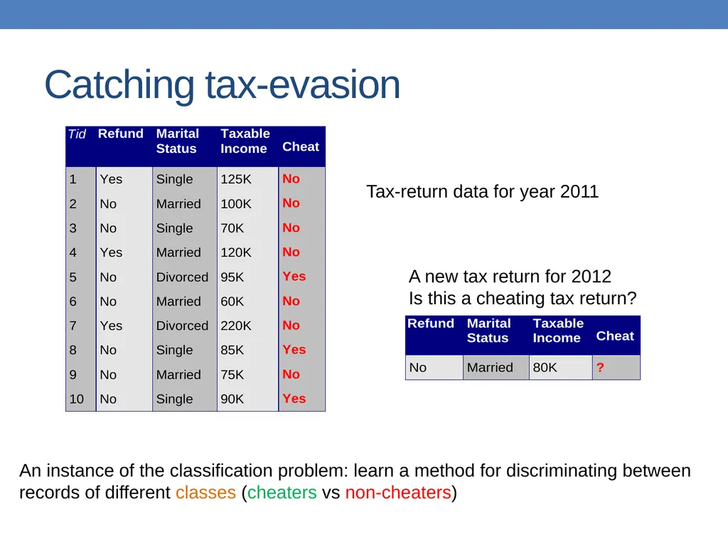
slide2. Catching tax-evasion Tax-return data for year 2011 A new tax return for 2012
Is this a cheating tax return? An instance of the classification problem: learn a method for discriminating between records of different classes (cheaters vs non-cheaters)<br>
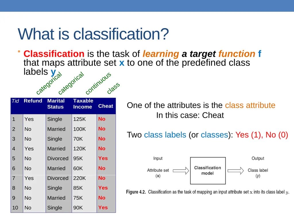
slide3. What is classification? Classification is the task of learning a target function f that maps attribute set x to one of the predefined class labels y One of the attributes is the class attribute
In this case: Cheat
Two class labels (or classes): Yes (1), No (0)<br>
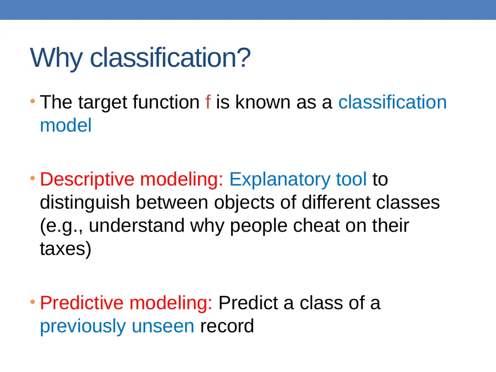
slide4. Why classification? The target function f is known as a classification model
Descriptive modeling: Explanatory tool to distinguish between objects of different classes (e.g., understand why people cheat on their taxes)
Predictive modeling: Predict a class of a previously unseen record<br>
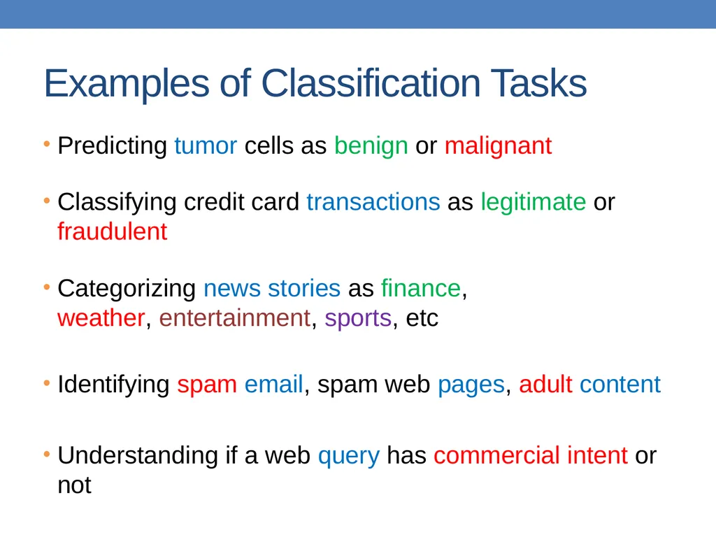
slide5. Examples of Classification Tasks Predicting tumor cells as benign or malignant
Classifying credit card transactions as legitimate or fraudulent
Categorizing news stories as finance, weather, entertainment, sports, etc
Identifying spam email, spam web pages, adult content
Understanding if a web query has commercial intent or not<br>
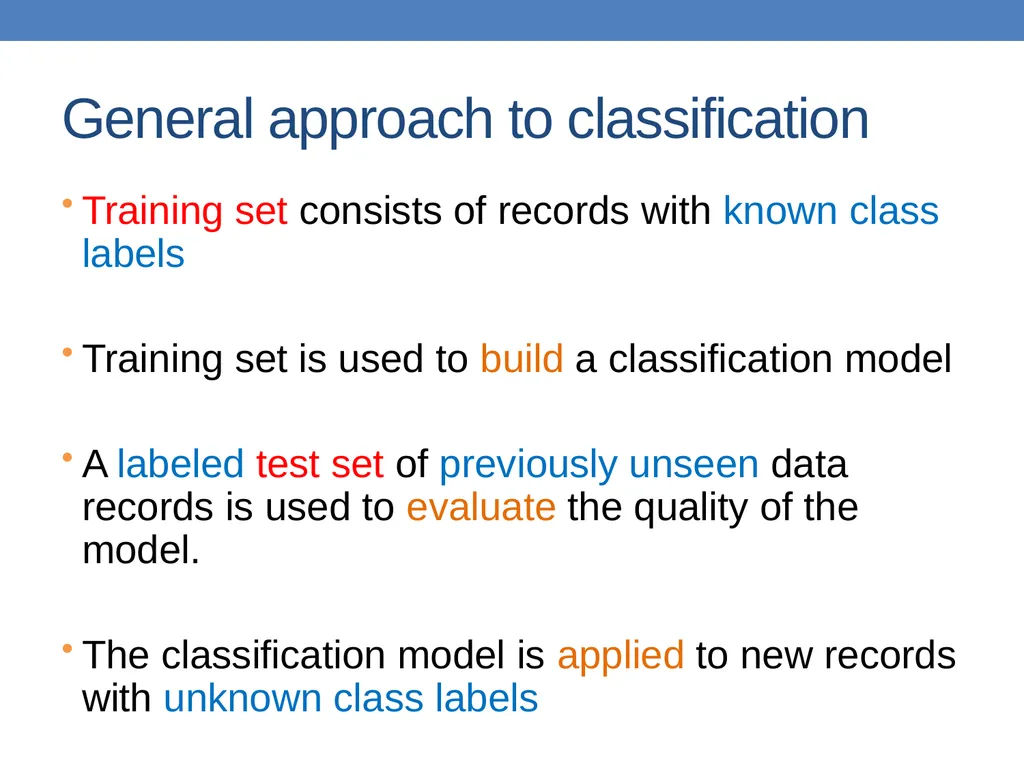
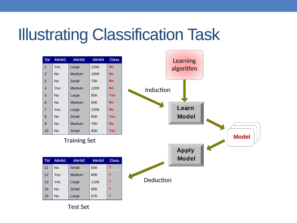
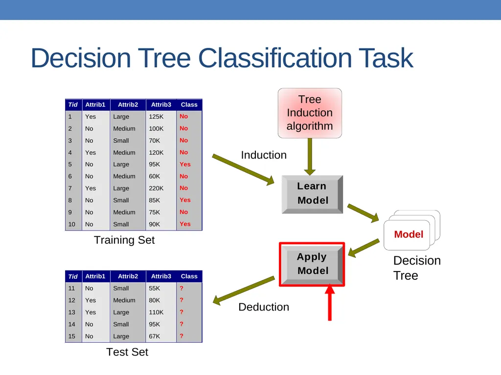
slide6. General approach to classification Training set consists of records with known class labels
Training set is used to build a classification model
A labeled test set of previously unseen data records is used to evaluate the quality of the model.
The classification model is applied to new records with unknown class labels<br>
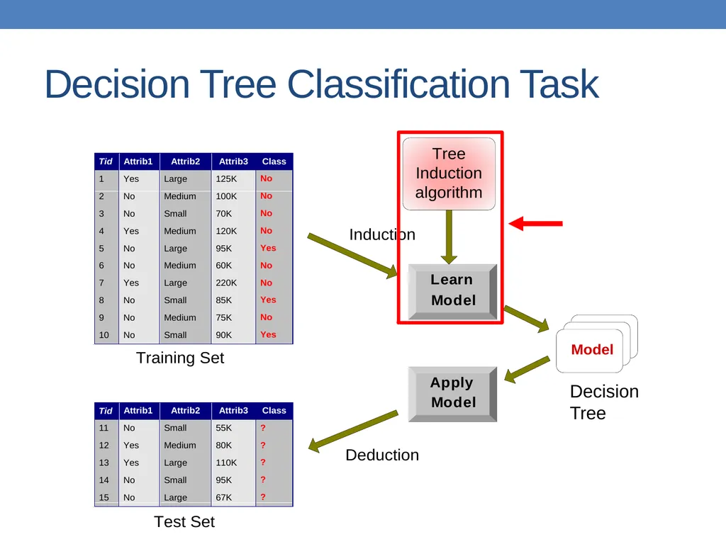
slide7. Illustrating Classification Task<br>
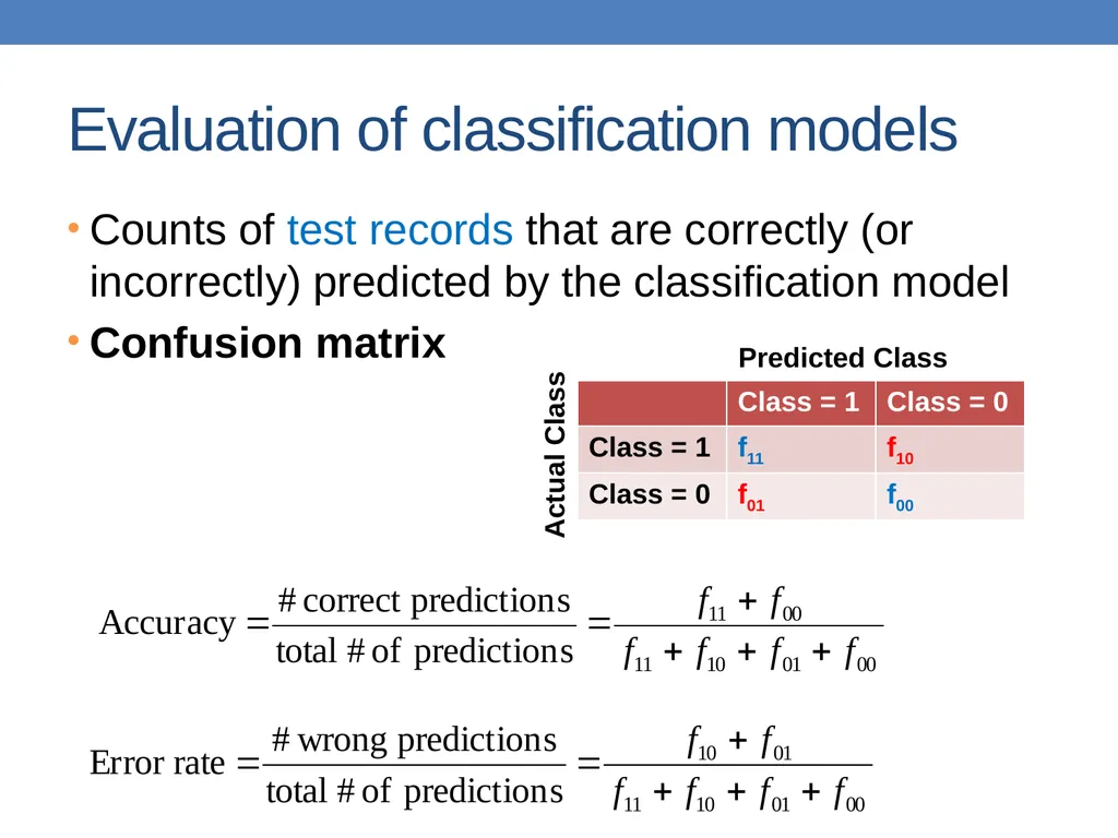
slide8. Evaluation of classification models Counts of test records that are correctly (or incorrectly) predicted by the classification model
Confusion matrix Predicted Class Actual Class<br>
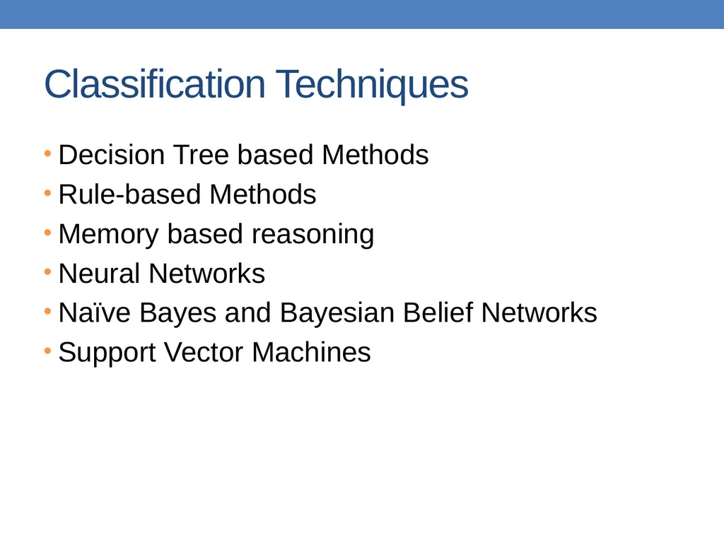
slide9. Classification Techniques Decision Tree based Methods
Rule-based Methods
Memory based reasoning
Neural Networks
Naïve Bayes and Bayesian Belief Networks
Support Vector Machines<br>
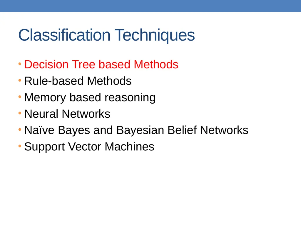
slide10. Classification Techniques Decision Tree based Methods
Rule-based Methods
Memory based reasoning
Neural Networks
Naïve Bayes and Bayesian Belief Networks
Support Vector Machines<br>
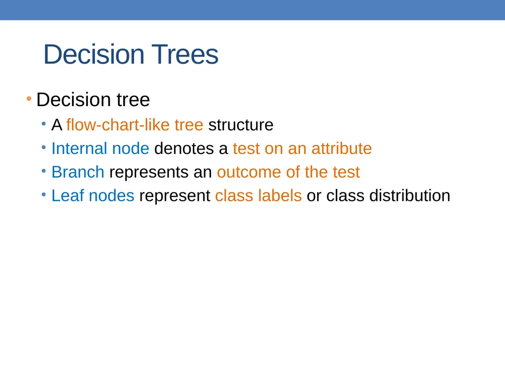
slide11. Decision Trees Decision tree
A flow-chart-like tree structure
Internal node denotes a test on an attribute
Branch represents an outcome of the test
Leaf nodes represent class labels or class distribution<br>
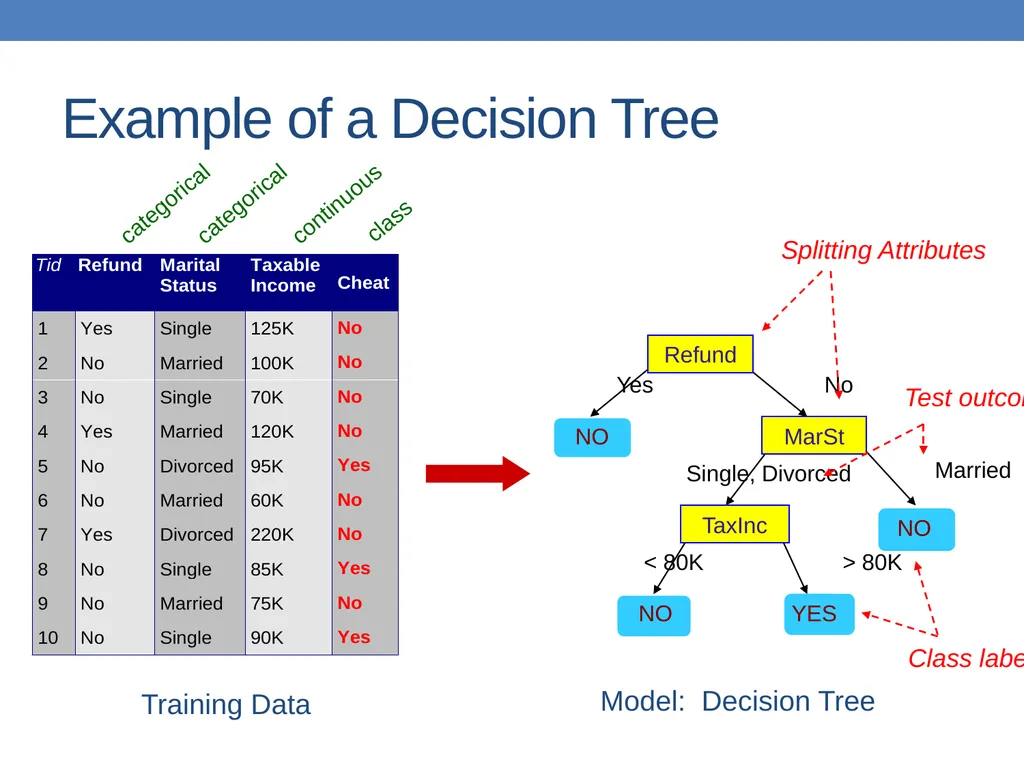
slide12. Example of a Decision Tree Refund MarSt TaxInc YES NO NO NO Yes No Married Single, Divorced < 80K > 80K Splitting Attributes Training Data Model: Decision Tree Test outcome Class labels<br>
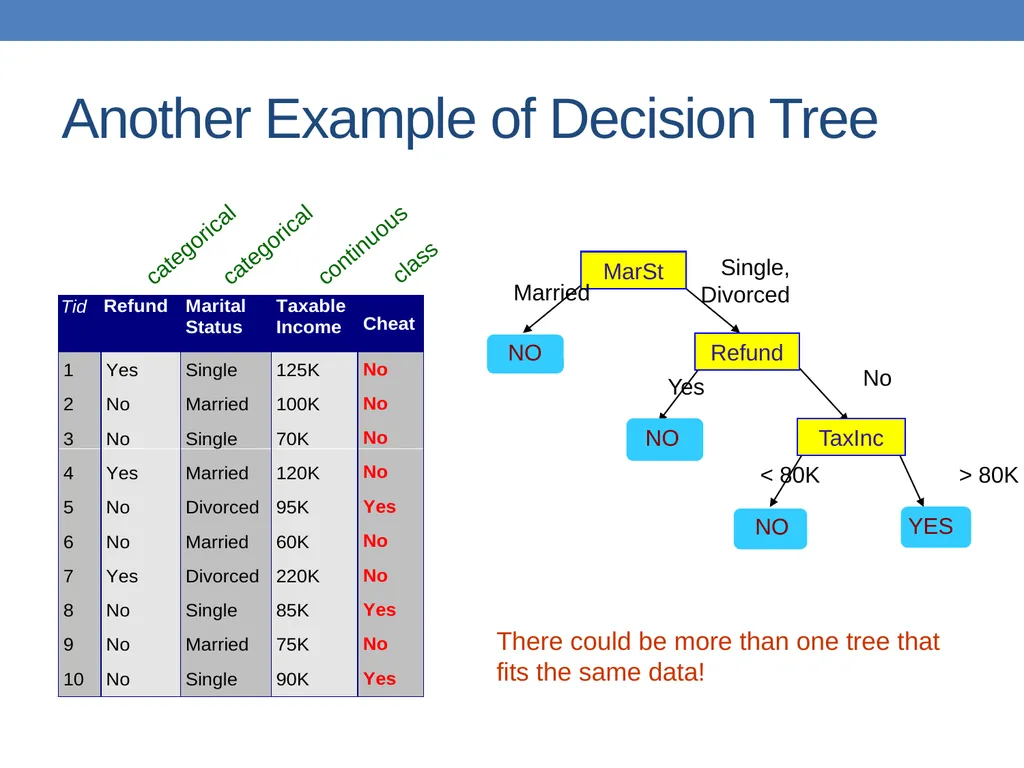
slide13. Another Example of Decision Tree categorical categorical continuous class MarSt Refund TaxInc YES NO NO Yes No Married Single, Divorced < 80K > 80K There could be more than one tree that fits the same data!<br>
slide14. Decision Tree Classification Task Decision Tree<br>
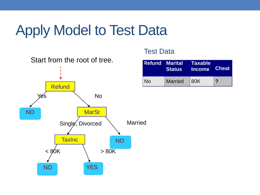
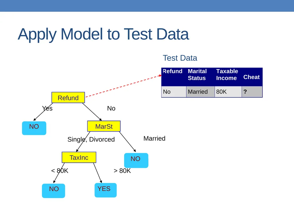
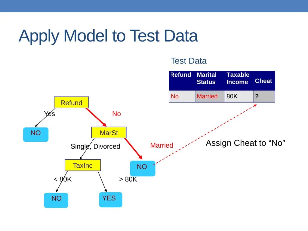
slide15. Apply Model to Test Data Test Data Start from the root of tree.<br>
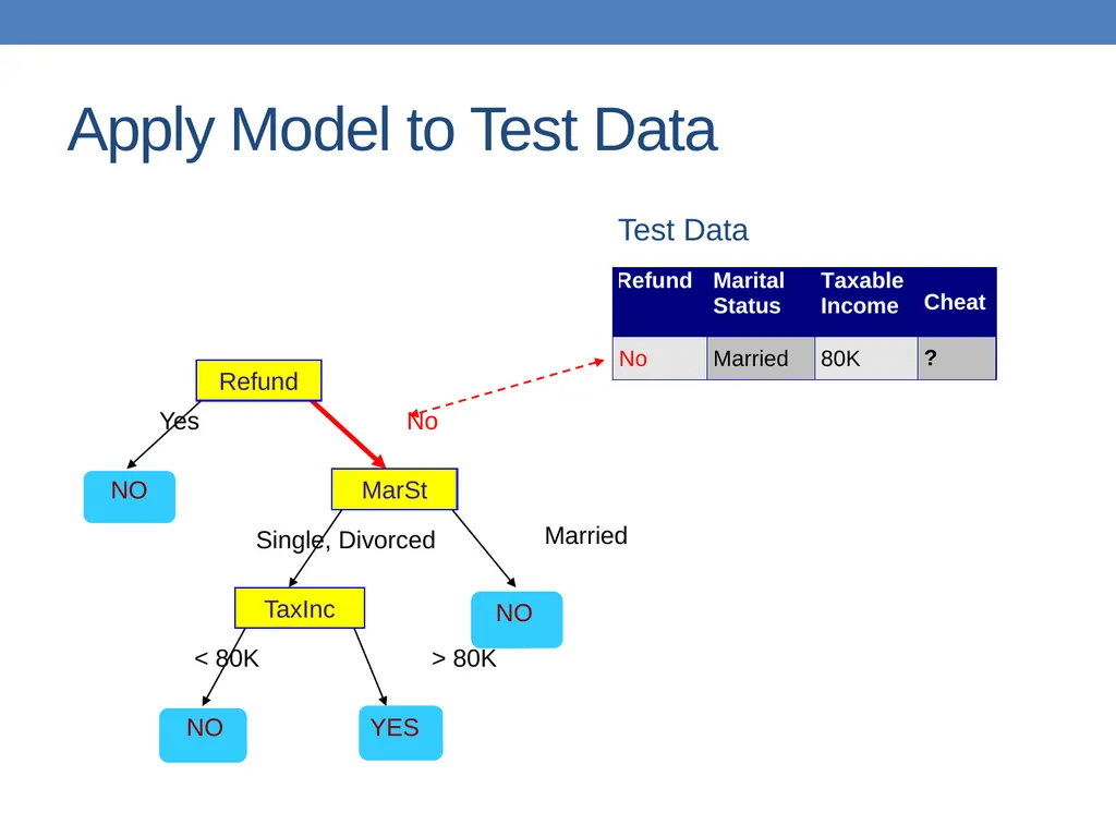
slide16. Apply Model to Test Data Test Data<br>
slide17. Apply Model to Test Data Refund MarSt TaxInc YES NO NO NO Yes No Married Single, Divorced < 80K > 80K Test Data<br>
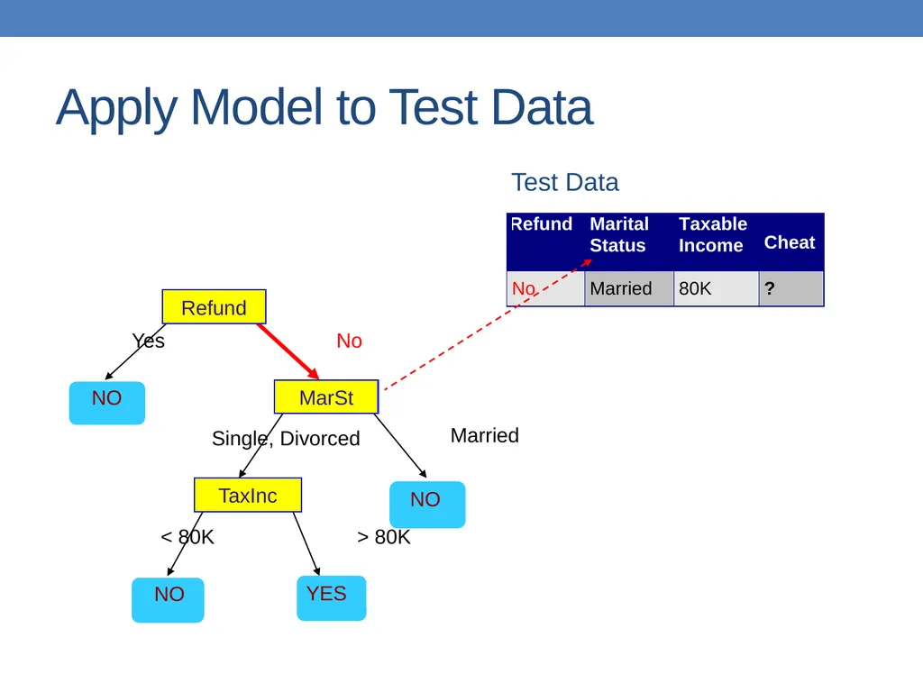
slide18. Apply Model to Test Data Refund MarSt TaxInc YES NO NO NO Yes No Married Single, Divorced < 80K > 80K Test Data<br>
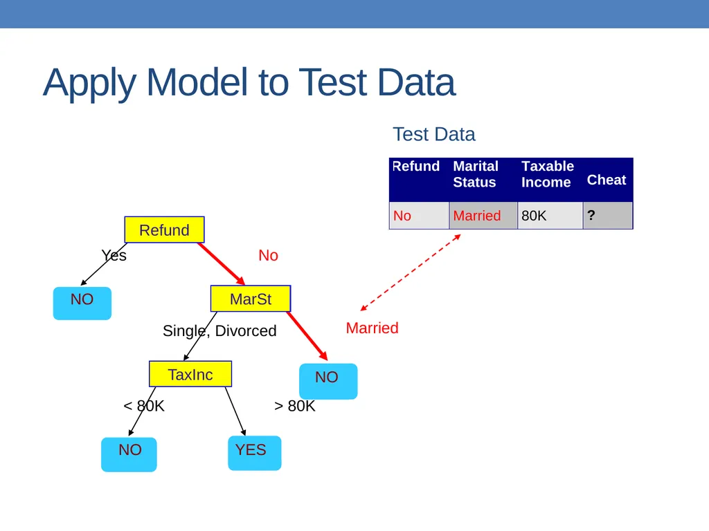
slide19. Apply Model to Test Data Refund MarSt TaxInc YES NO NO NO Yes No Married Single, Divorced < 80K > 80K Test Data<br>
slide20. Apply Model to Test Data Refund MarSt TaxInc YES NO NO NO Yes No Married Single, Divorced < 80K > 80K Test Data Assign Cheat to “No”<br>
slide21. Decision Tree Classification Task Decision Tree<br>
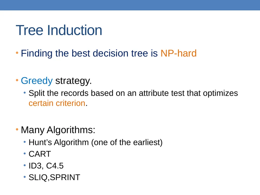
slide22. Tree Induction Finding the best decision tree is NP-hard
Greedy strategy.
Split the records based on an attribute test that optimizes certain criterion.
Many Algorithms:
Hunt’s Algorithm (one of the earliest)
CART
ID3, C4.5
SLIQ,SPRINT<br>
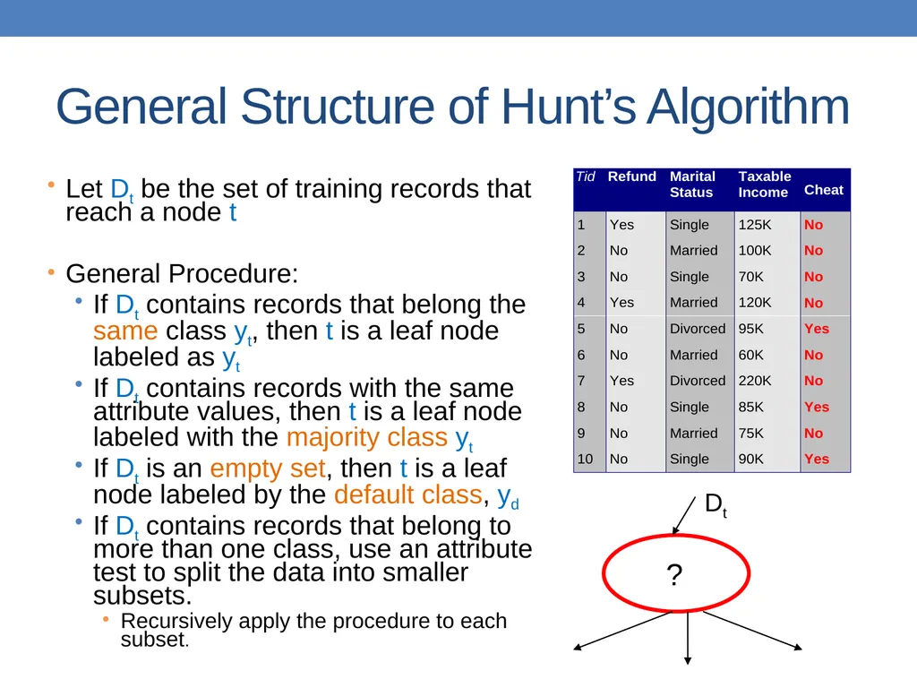
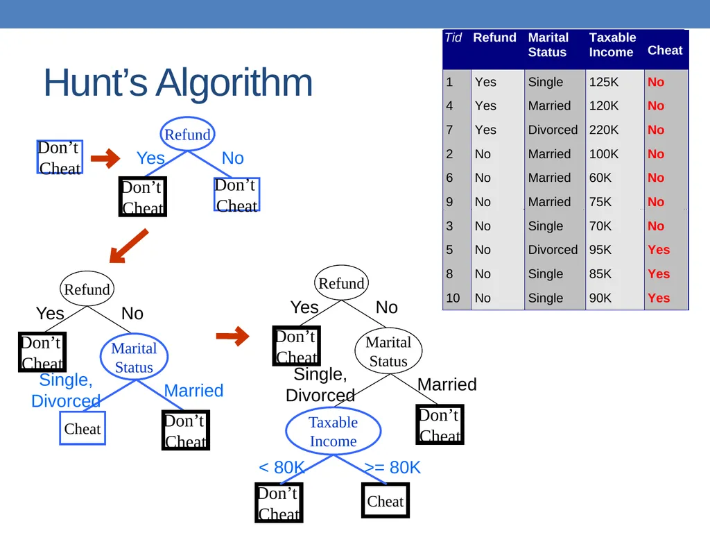
slide23. General Structure of Hunt’s Algorithm Let Dt be the set of training records that reach a node t
General Procedure:
If Dt contains records that belong the same class yt, then t is a leaf node labeled as yt
If Dt contains records with the same attribute values, then t is a leaf node labeled with the majority class yt
If Dt is an empty set, then t is a leaf node labeled by the default class, yd
If Dt contains records that belong to more than one class, use an attribute test to split the data into smaller subsets.
Recursively apply the procedure to each subset. Dt ?<br>
slide24. Hunt’s Algorithm Don’t
Cheat<br>
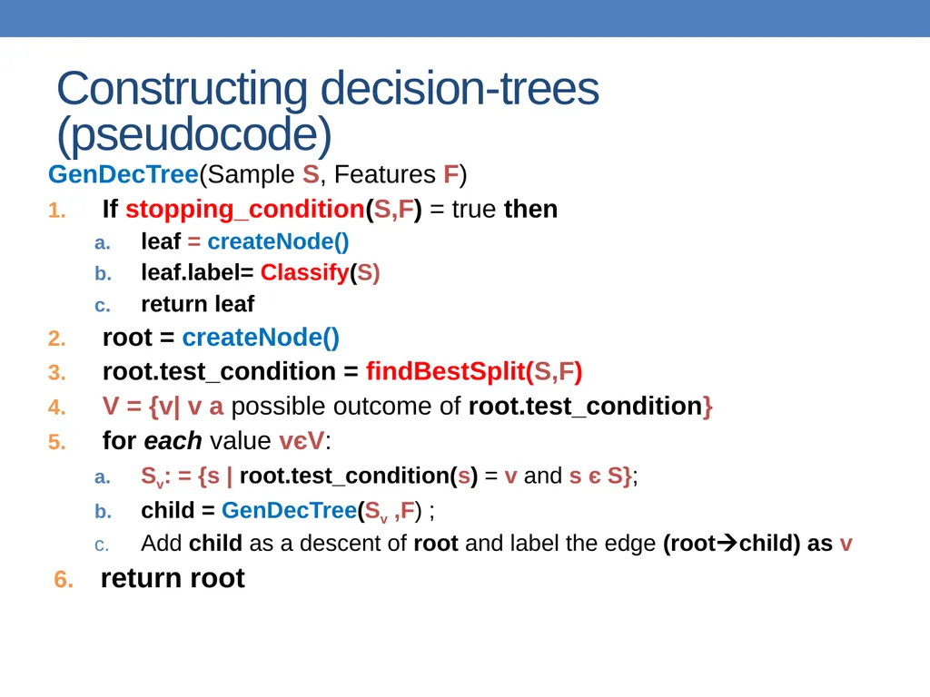
slide25. Constructing decision-trees (pseudocode) GenDecTree(Sample S, Features F)
If stopping_condition(S,F) = true then
leaf = createNode()
leaf.label= Classify(S)
return leaf
root = createNode()
root.test_condition = findBestSplit(S,F)
V = {v| v a possible outcome of root.test_condition}
for each value vєV:
Sv: = {s | root.test_condition(s) = v and s є S};
child = GenDecTree(Sv ,F) ;
Add child as a descent of root and label the edge (rootchild) as v
return root<br>
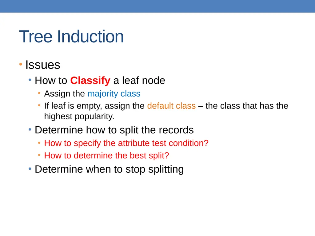
slide26. Tree Induction Issues
How to Classify a leaf node
Assign the majority class
If leaf is empty, assign the default class – the class that has the highest popularity.
Determine how to split the records
How to specify the attribute test condition?
How to determine the best split?
Determine when to stop splitting<br>
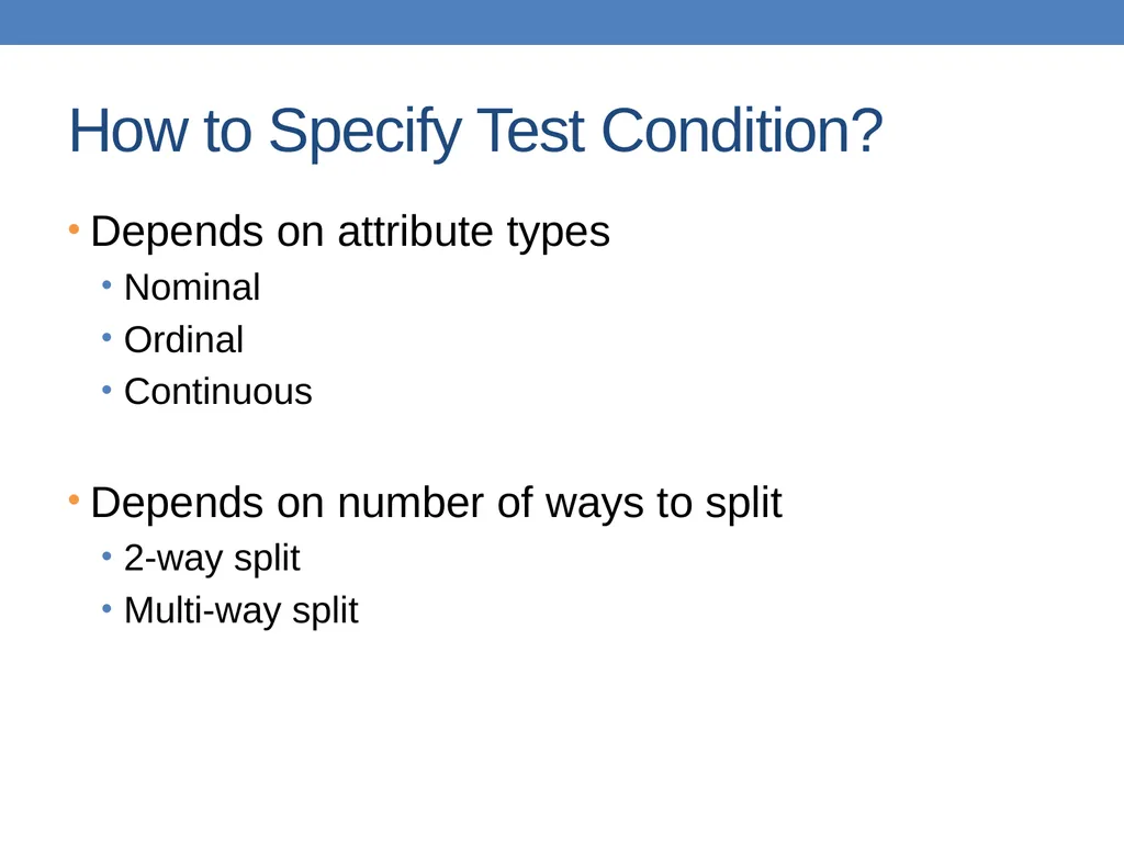
slide27. How to Specify Test Condition? Depends on attribute types
Nominal
Ordinal
Continuous
Depends on number of ways to split
2-way split
Multi-way split<br>
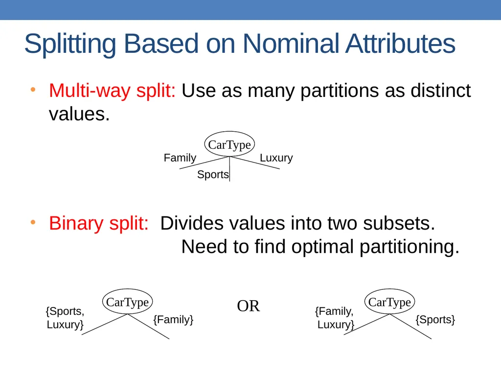
slide28. Splitting Based on Nominal Attributes Multi-way split: Use as many partitions as distinct values.
Binary split: Divides values into two subsets. Need to find optimal partitioning. OR<br>
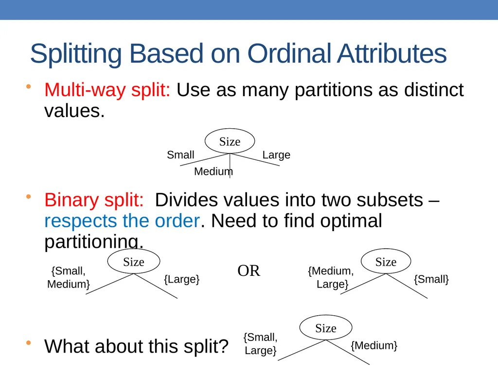
slide29. Multi-way split: Use as many partitions as distinct values.
Binary split: Divides values into two subsets – respects the order. Need to find optimal partitioning.
What about this split? Splitting Based on Ordinal Attributes OR<br>
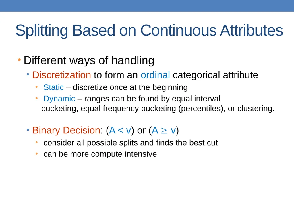
slide30. Splitting Based on Continuous Attributes Different ways of handling
Discretization to form an ordinal categorical attribute
Static – discretize once at the beginning
Dynamic – ranges can be found by equal interval bucketing, equal frequency bucketing (percentiles), or clustering.
Binary Decision: (A < v) or (A v)
consider all possible splits and finds the best cut
can be more compute intensive<br>
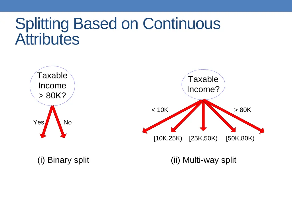
slide31. Splitting Based on Continuous Attributes<br>
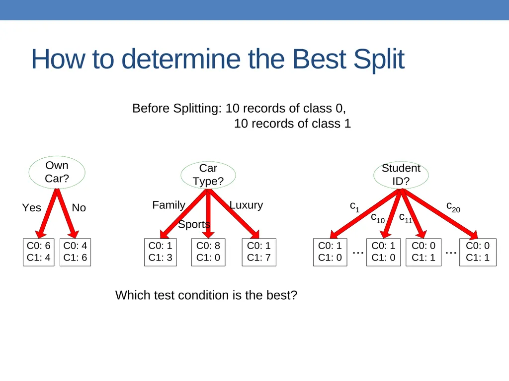
slide32. How to determine the Best Split Before Splitting: 10 records of class 0, 10 records of class 1 Which test condition is the best?<br>
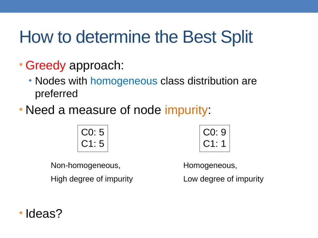
slide33. How to determine the Best Split Greedy approach:
Nodes with homogeneous class distribution are preferred
Need a measure of node impurity:
Ideas? Non-homogeneous,
High degree of impurity Homogeneous,
Low degree of impurity<br>
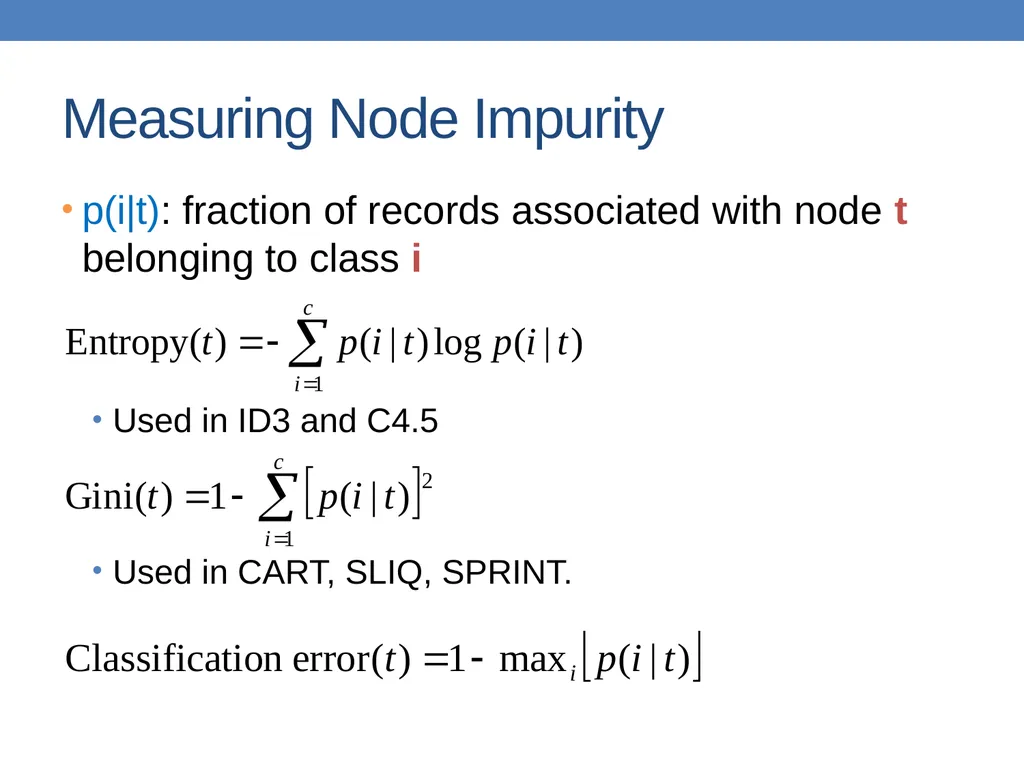
slide34. Measuring Node Impurity p(i|t): fraction of records associated with node t belonging to class i
Used in ID3 and C4.5
Used in CART, SLIQ, SPRINT.<br>
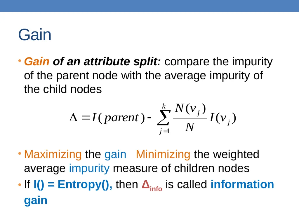
slide35. Gain Gain of an attribute split: compare the impurity of the parent node with the average impurity of the child nodes
Maximizing the gain Minimizing the weighted average impurity measure of children nodes
If I() = Entropy(), then Δinfo is called information gain<br>
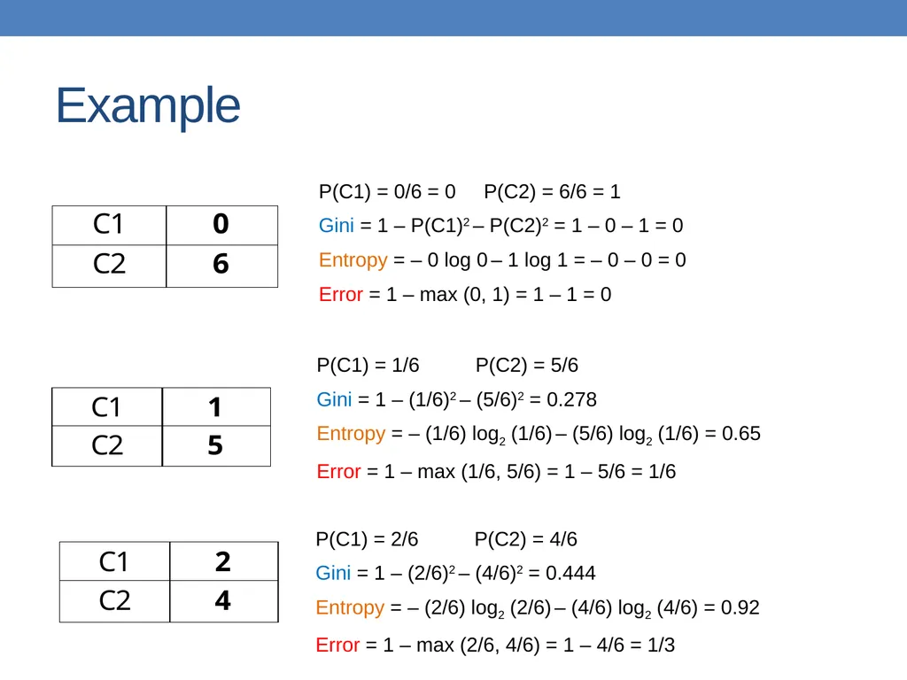
slide36. Example P(C1) = 0/6 = 0 P(C2) = 6/6 = 1
Gini = 1 – P(C1)2 – P(C2)2 = 1 – 0 – 1 = 0
Entropy = – 0 log 0 – 1 log 1 = – 0 – 0 = 0
Error = 1 – max (0, 1) = 1 – 1 = 0 P(C1) = 1/6 P(C2) = 5/6
Gini = 1 – (1/6)2 – (5/6)2 = 0.278
Entropy = – (1/6) log2 (1/6) – (5/6) log2 (1/6) = 0.65
Error = 1 – max (1/6, 5/6) = 1 – 5/6 = 1/6 P(C1) = 2/6 P(C2) = 4/6
Gini = 1 – (2/6)2 – (4/6)2 = 0.444
Entropy = – (2/6) log2 (2/6) – (4/6) log2 (4/6) = 0.92
Error = 1 – max (2/6, 4/6) = 1 – 4/6 = 1/3<br>
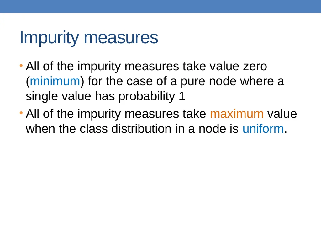
slide37. Impurity measures All of the impurity measures take value zero (minimum) for the case of a pure node where a single value has probability 1
All of the impurity measures take maximum value when the class distribution in a node is uniform.<br>
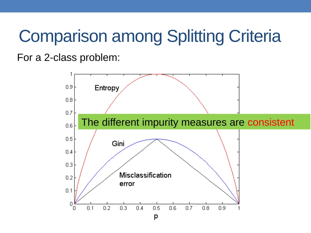
slide38. Comparison among Splitting Criteria For a 2-class problem: The different impurity measures are consistent<br>
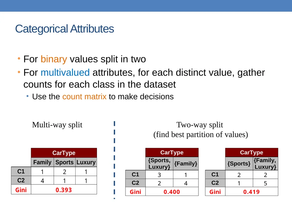
slide39. Categorical Attributes For binary values split in two
For multivalued attributes, for each distinct value, gather counts for each class in the dataset
Use the count matrix to make decisions Multi-way split Two-way split
(find best partition of values)<br>
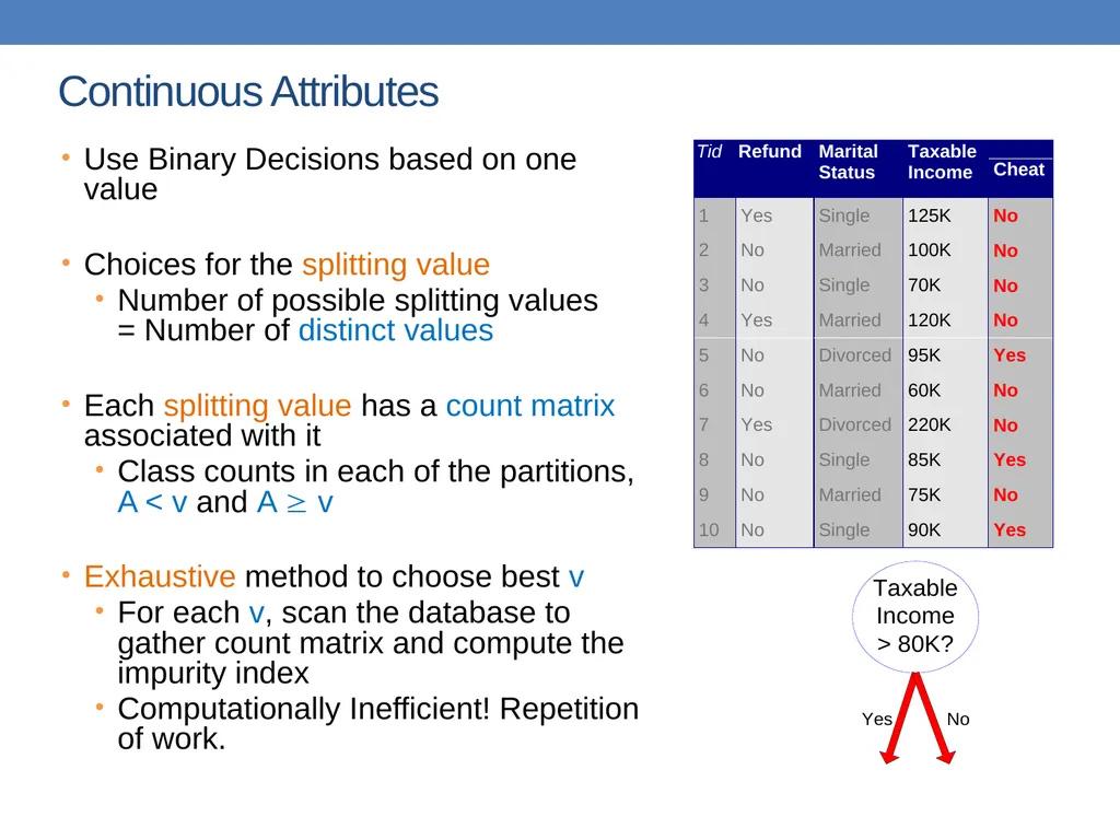
slide40. Continuous Attributes Use Binary Decisions based on one value
Choices for the splitting value
Number of possible splitting values = Number of distinct values
Each splitting value has a count matrix associated with it
Class counts in each of the partitions, A < v and A v
Exhaustive method to choose best v
For each v, scan the database to gather count matrix and compute the impurity index
Computationally Inefficient! Repetition of work.<br>
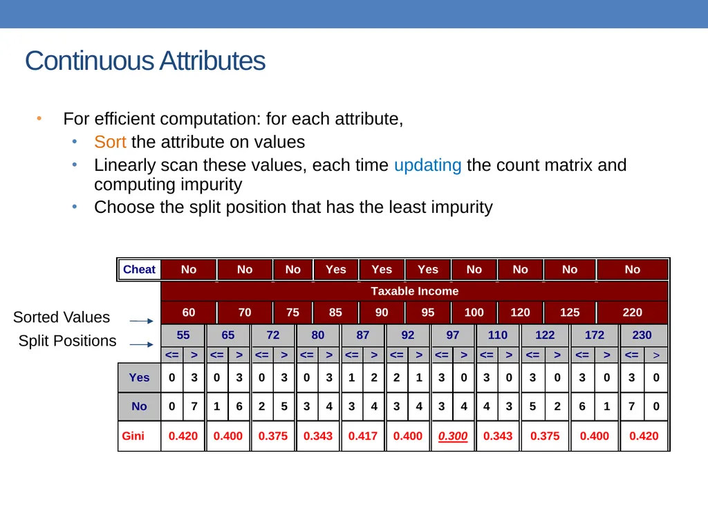
slide41. Continuous Attributes For efficient computation: for each attribute,
Sort the attribute on values
Linearly scan these values, each time updating the count matrix and computing impurity
Choose the split position that has the least impurity<br>
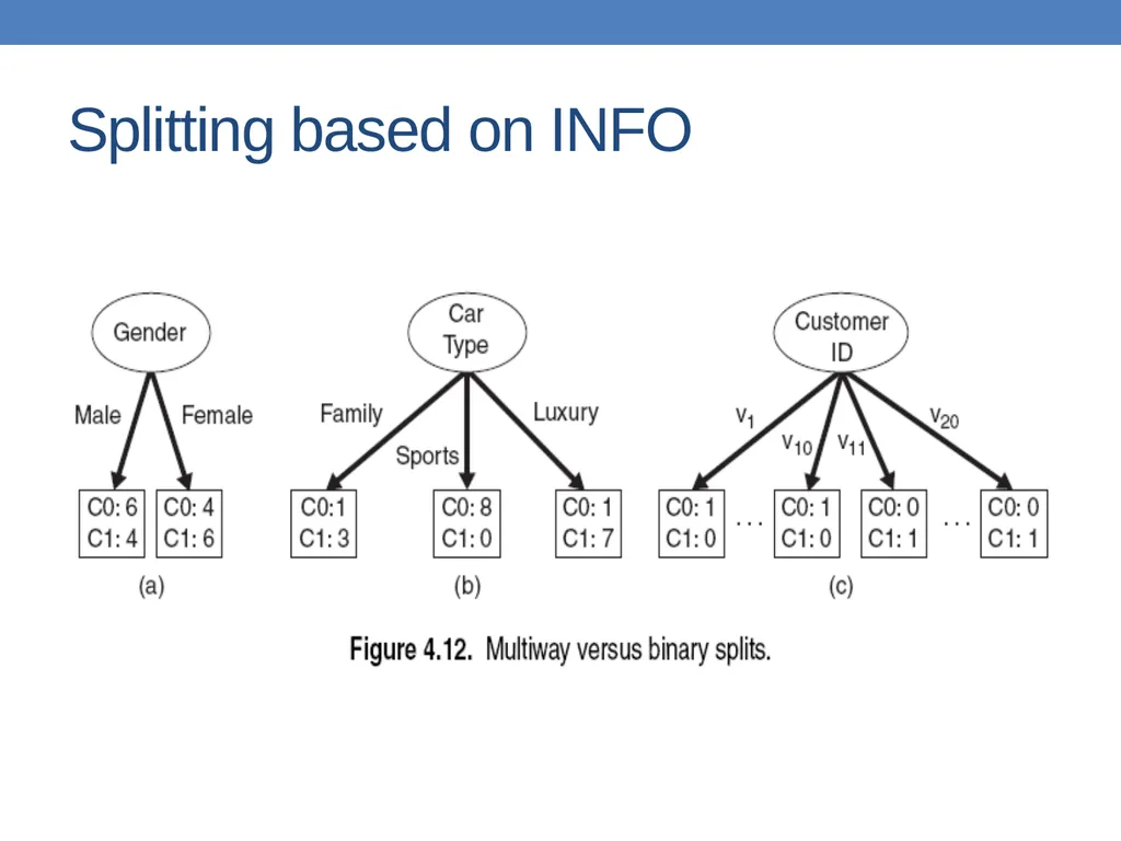
slide42. Splitting based on impurity Impurity measures favor attributes with large number of values
A test condition with large number of outcomes may not be desirable
# of records in each partition is too small to make predictions<br>
slide43. Splitting based on INFO<br>
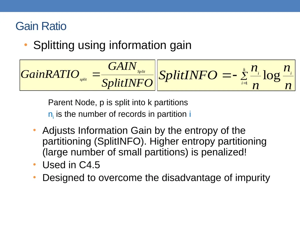
slide44. Gain Ratio Splitting using information gain
Parent Node, p is split into k partitions
ni is the number of records in partition i
Adjusts Information Gain by the entropy of the partitioning (SplitINFO). Higher entropy partitioning (large number of small partitions) is penalized!
Used in C4.5
Designed to overcome the disadvantage of impurity<br>
slide45. Stopping Criteria for Tree Induction Stop expanding a node when all the records belong to the same class
Stop expanding a node when all the records have similar attribute values
Early termination (to be discussed later)<br>
slide46. Decision Tree Based Classification Advantages:
Inexpensive to construct
Extremely fast at classifying unknown records
Easy to interpret for small-sized trees
Accuracy is comparable to other classification techniques for many simple data sets<br>
slide47. Example: C4.5 Simple depth-first construction.
Uses Information Gain
Sorts Continuous Attributes at each node.
Needs entire data to fit in memory.
Unsuitable for Large Datasets.
Needs out-of-core sorting.
You can download the software from: http://www.cse.unsw.edu.au/~quinlan/c4.5r8.tar.gz<br>
slide48. Other Issues Data Fragmentation
Expressiveness<br>
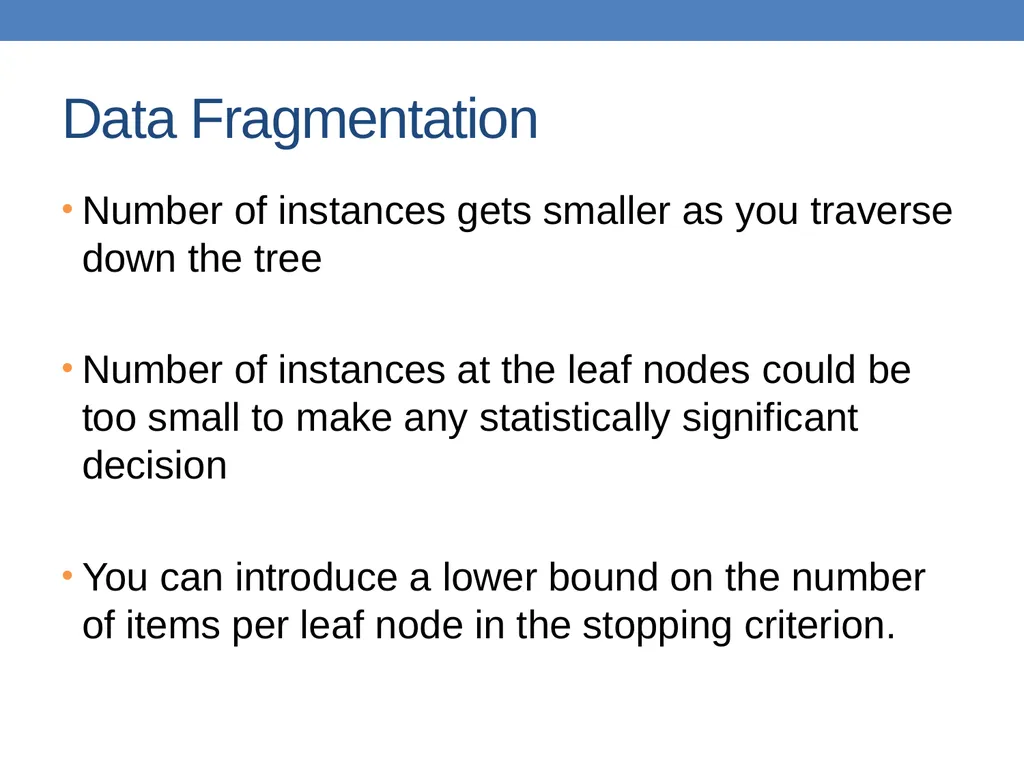
slide49. Data Fragmentation Number of instances gets smaller as you traverse down the tree
Number of instances at the leaf nodes could be too small to make any statistically significant decision
You can introduce a lower bound on the number of items per leaf node in the stopping criterion.<br>
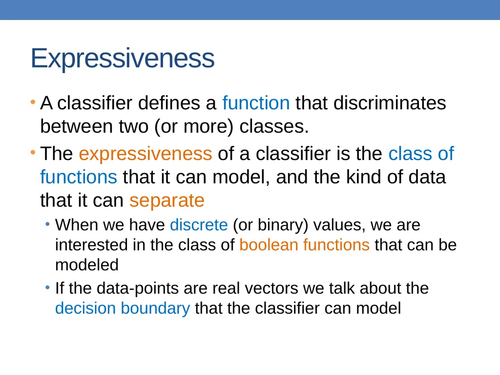
slide50. Expressiveness A classifier defines a function that discriminates between two (or more) classes.
The expressiveness of a classifier is the class of functions that it can model, and the kind of data that it can separate
When we have discrete (or binary) values, we are interested in the class of boolean functions that can be modeled
If the data-points are real vectors we talk about the decision boundary that the classifier can model<br>
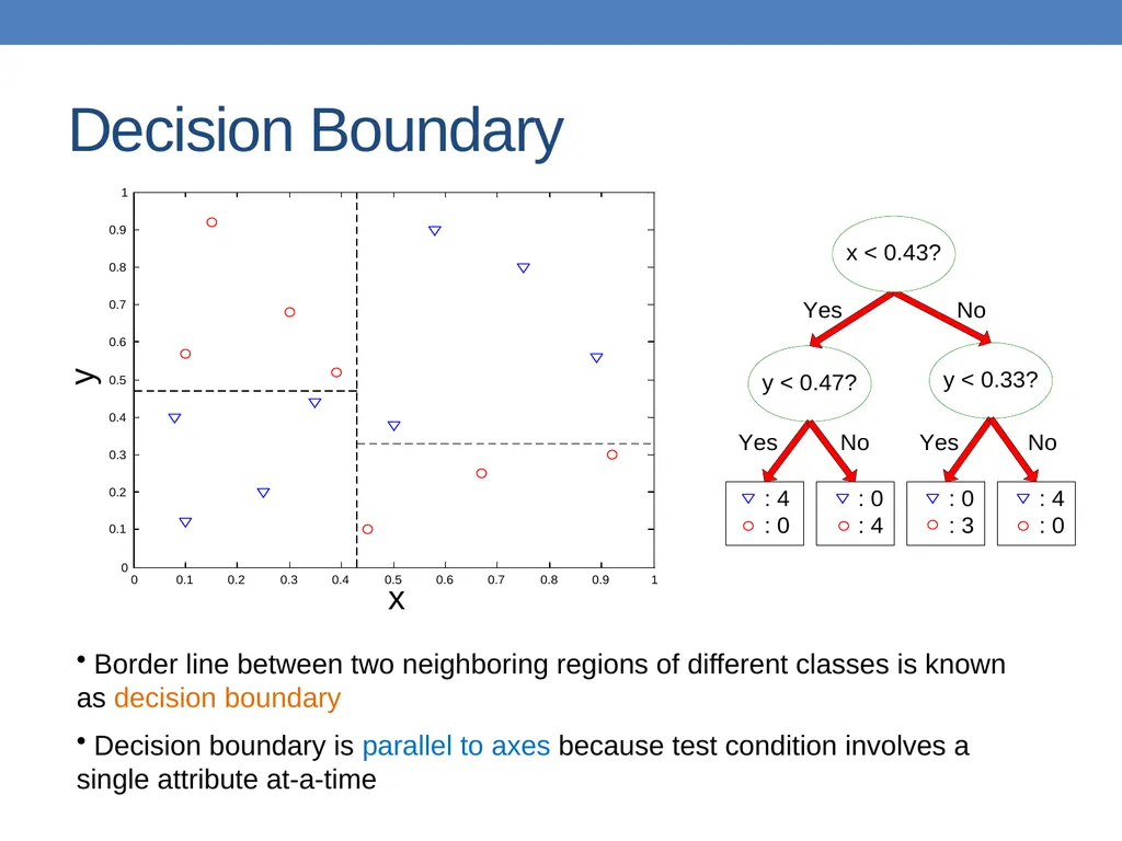
slide51. Decision Boundary Border line between two neighboring regions of different classes is known as decision boundary
Decision boundary is parallel to axes because test condition involves a single attribute at-a-time<br>
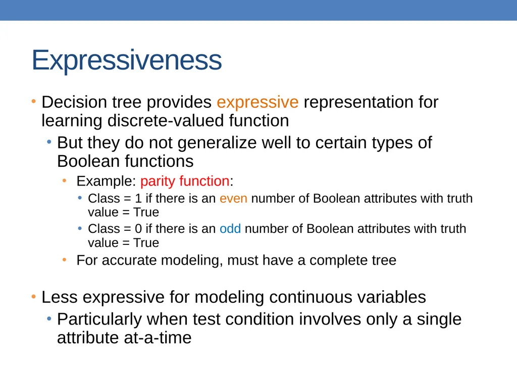
slide52. Expressiveness Decision tree provides expressive representation for learning discrete-valued function
But they do not generalize well to certain types of Boolean functions
Example: parity function:
Class = 1 if there is an even number of Boolean attributes with truth value = True
Class = 0 if there is an odd number of Boolean attributes with truth value = True
For accurate modeling, must have a complete tree
Less expressive for modeling continuous variables
Particularly when test condition involves only a single attribute at-a-time<br>
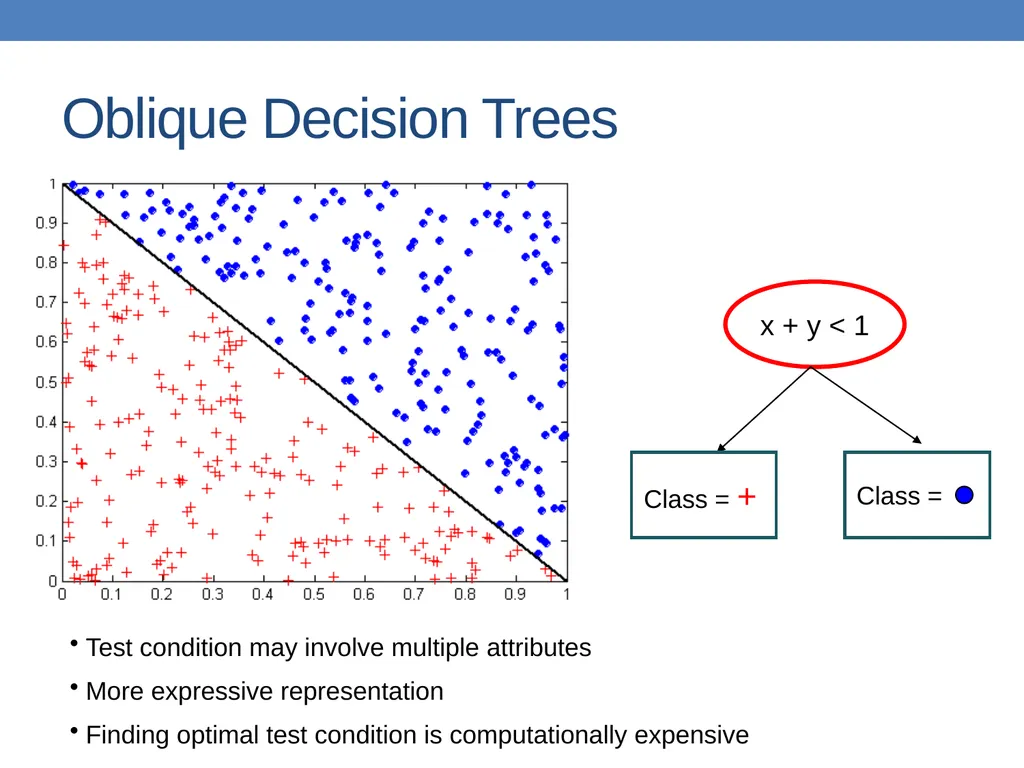
slide53. Oblique Decision Trees Test condition may involve multiple attributes
More expressive representation
Finding optimal test condition is computationally expensive<br>
slide54. Practical Issues of Classification Underfitting and Overfitting
Evaluation<br>
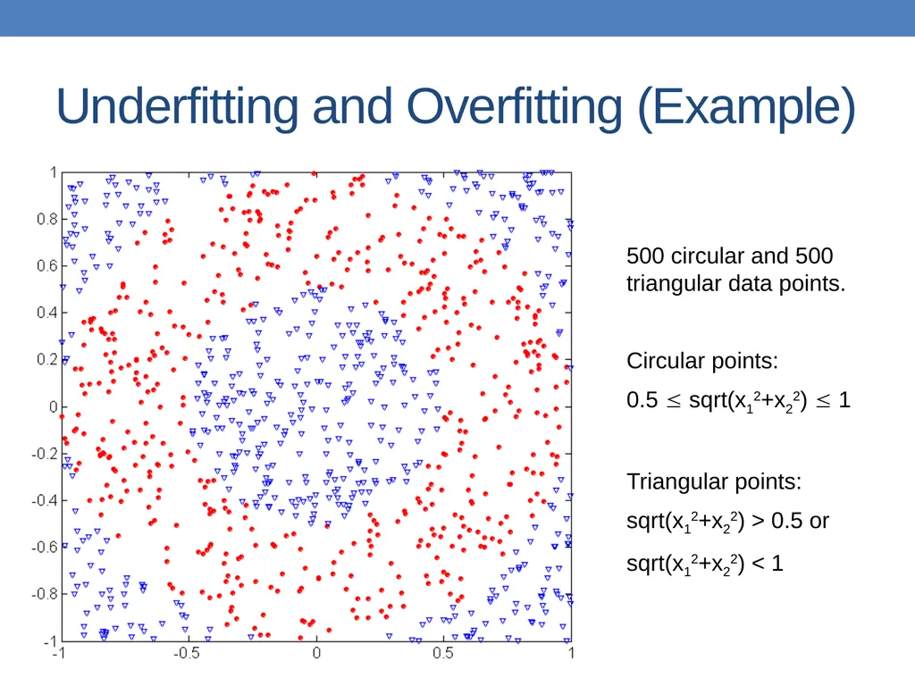
slide55. Underfitting and Overfitting (Example) 500 circular and 500 triangular data points.
Circular points:
0.5 sqrt(x12+x22) 1
Triangular points:
sqrt(x12+x22) > 0.5 or
sqrt(x12+x22) < 1<br>
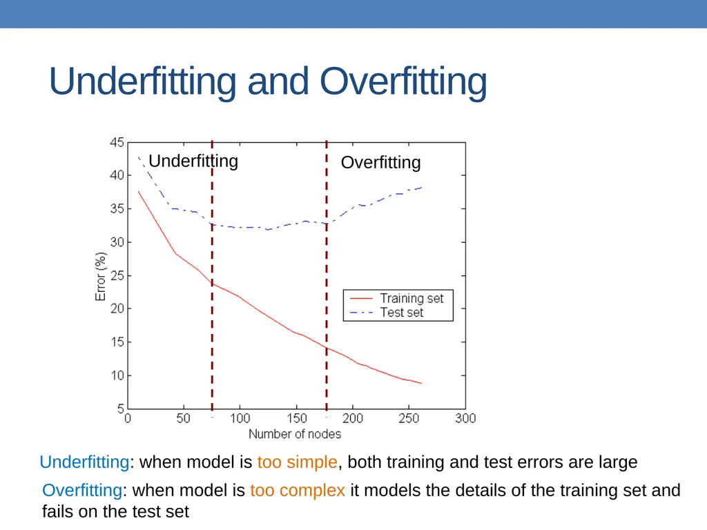
slide56. Underfitting and Overfitting Overfitting Underfitting: when model is too simple, both training and test errors are large Underfitting Overfitting: when model is too complex it models the details of the training set and fails on the test set<br>
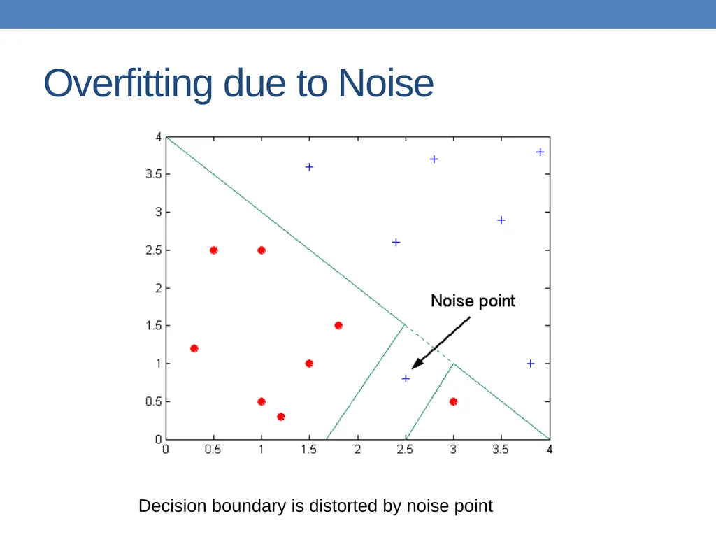
slide57. Overfitting due to Noise Decision boundary is distorted by noise point<br>
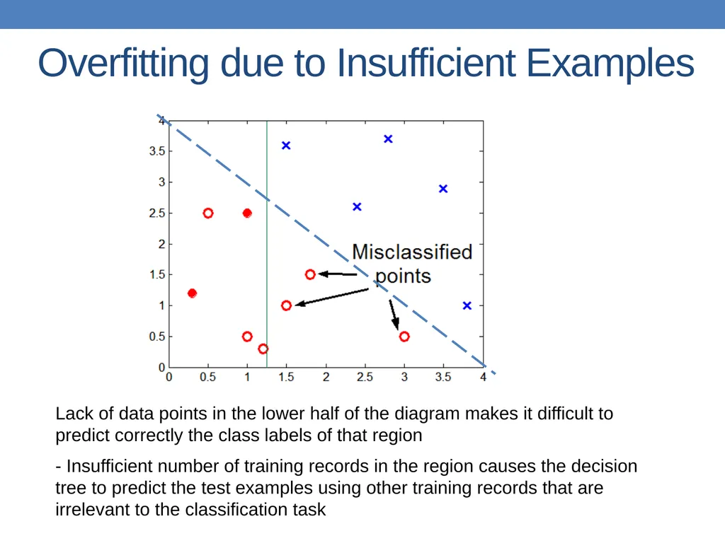
slide58. Overfitting due to Insufficient Examples Lack of data points in the lower half of the diagram makes it difficult to predict correctly the class labels of that region
- Insufficient number of training records in the region causes the decision tree to predict the test examples using other training records that are irrelevant to the classification task<br>
slide59. Notes on Overfitting Overfitting results in decision trees that are more complex than necessary
Training error no longer provides a good estimate of how well the tree will perform on previously unseen records
The model does not generalize well
Need new ways for estimating errors<br>
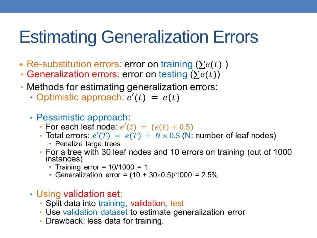
slide60. Estimating Generalization Errors<br>
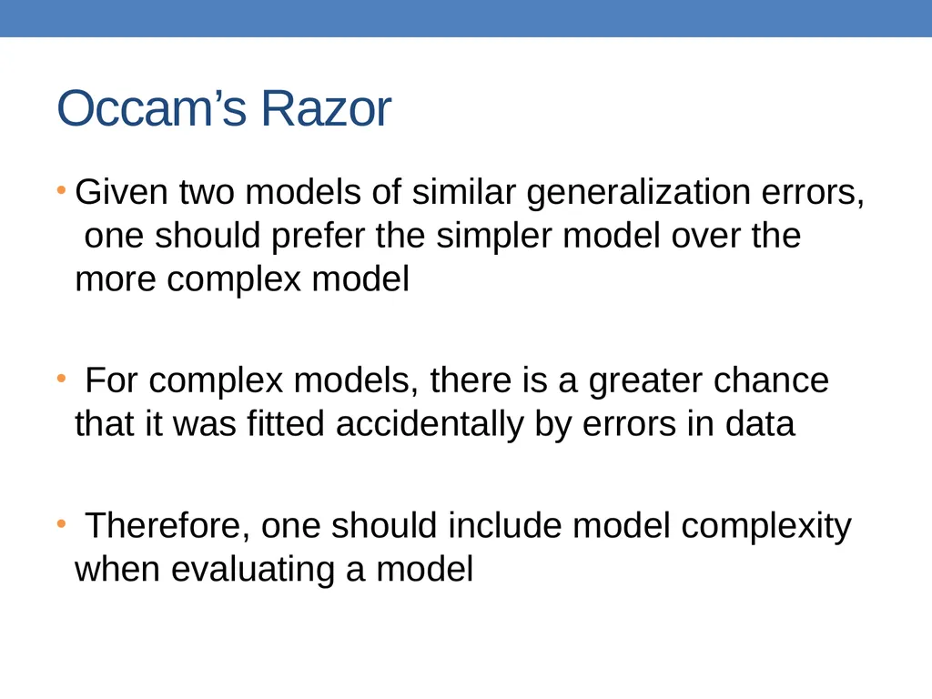
slide61. Occam’s Razor Given two models of similar generalization errors, one should prefer the simpler model over the more complex model
For complex models, there is a greater chance that it was fitted accidentally by errors in data
Therefore, one should include model complexity when evaluating a model<br>
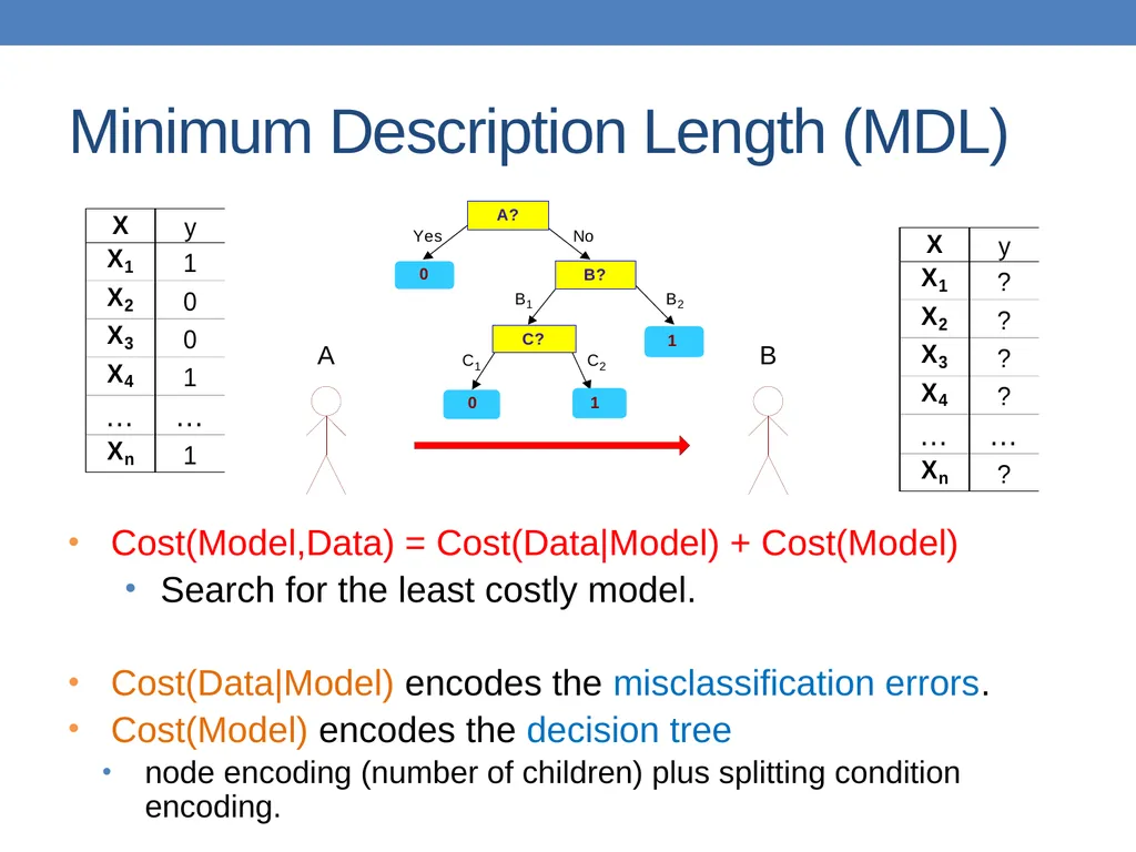
slide62. Minimum Description Length (MDL) Cost(Model,Data) = Cost(Data|Model) + Cost(Model)
Search for the least costly model.
Cost(Data|Model) encodes the misclassification errors.
Cost(Model) encodes the decision tree
node encoding (number of children) plus splitting condition encoding.<br>
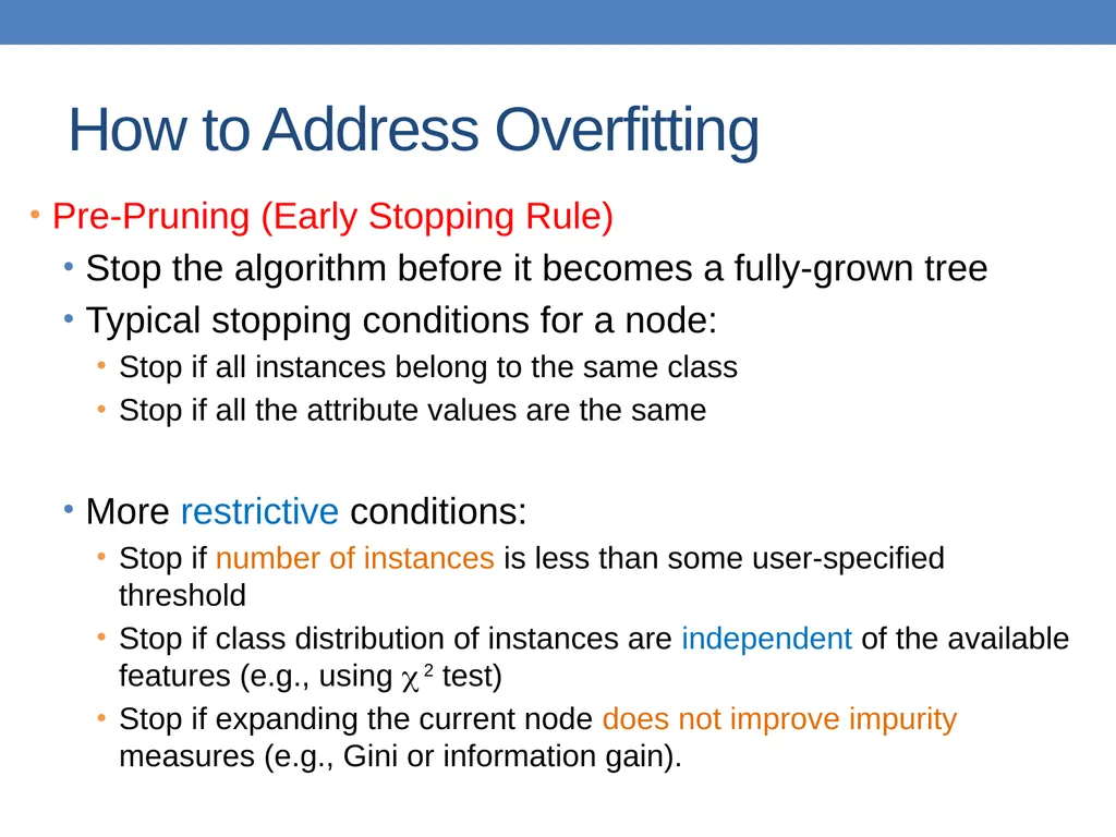
slide63. How to Address Overfitting Pre-Pruning (Early Stopping Rule)
Stop the algorithm before it becomes a fully-grown tree
Typical stopping conditions for a node:
Stop if all instances belong to the same class
Stop if all the attribute values are the same
More restrictive conditions:
Stop if number of instances is less than some user-specified threshold
Stop if class distribution of instances are independent of the available features (e.g., using 2 test)
Stop if expanding the current node does not improve impurity measures (e.g., Gini or information gain).<br>
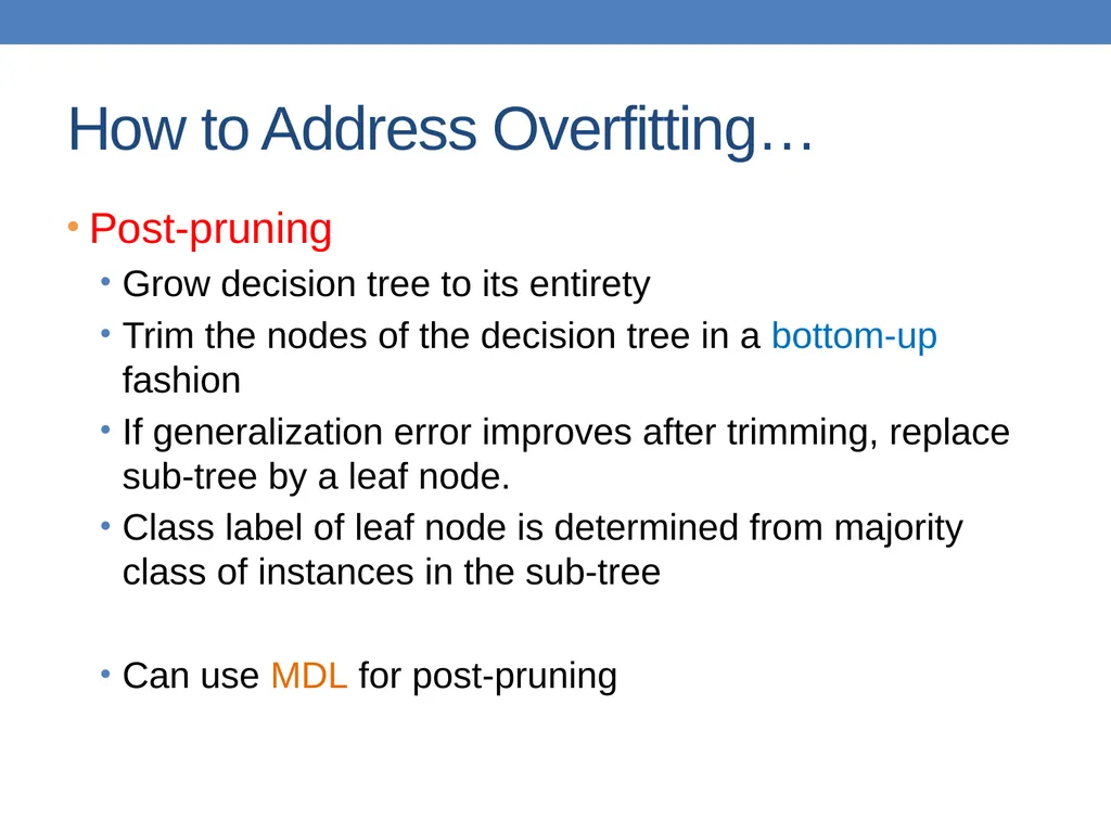
slide64. How to Address Overfitting… Post-pruning
Grow decision tree to its entirety
Trim the nodes of the decision tree in a bottom-up fashion
If generalization error improves after trimming, replace sub-tree by a leaf node.
Class label of leaf node is determined from majority class of instances in the sub-tree
Can use MDL for post-pruning<br>
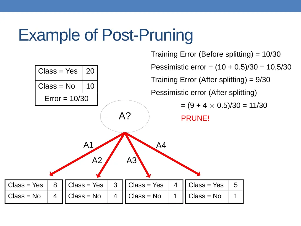
slide65. Example of Post-Pruning Training Error (Before splitting) = 10/30
Pessimistic error = (10 + 0.5)/30 = 10.5/30
Training Error (After splitting) = 9/30
Pessimistic error (After splitting)
= (9 + 4 0.5)/30 = 11/30
PRUNE!<br>
slide66. Model Evaluation Metrics for Performance Evaluation
How to evaluate the performance of a model?
Methods for Performance Evaluation
How to obtain reliable estimates?
Methods for Model Comparison
How to compare the relative performance among competing models?<br>
slide67. Model Evaluation Metrics for Performance Evaluation
How to evaluate the performance of a model?
Methods for Performance Evaluation
How to obtain reliable estimates?
Methods for Model Comparison
How to compare the relative performance among competing models?<br>
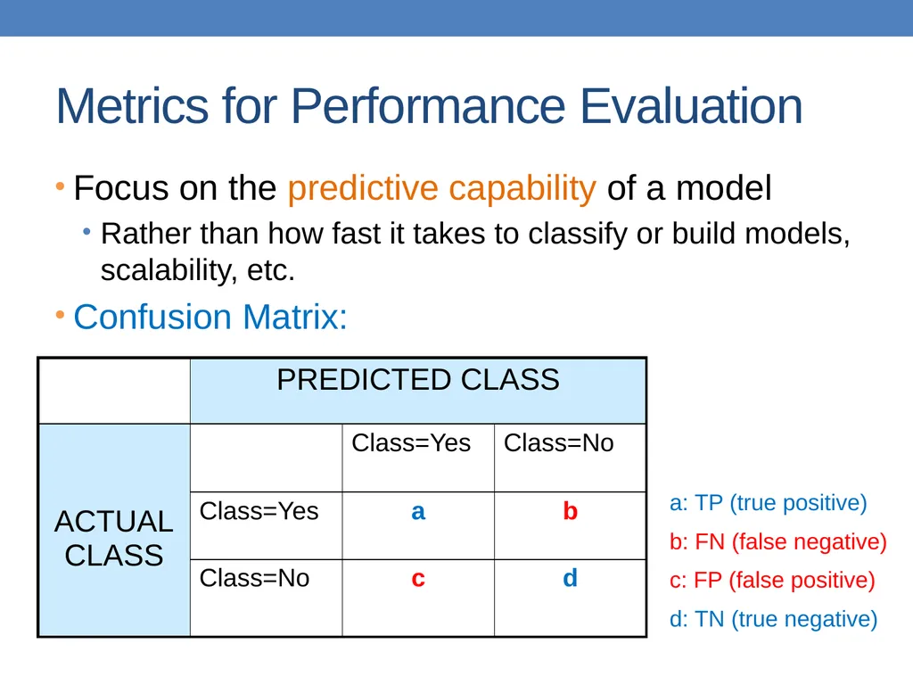
slide68. Metrics for Performance Evaluation Focus on the predictive capability of a model
Rather than how fast it takes to classify or build models, scalability, etc.
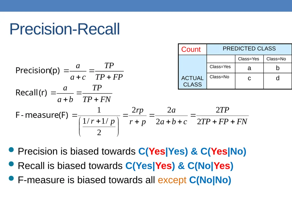
Confusion Matrix: a: TP (true positive)
b: FN (false negative)
c: FP (false positive)
d: TN (true negative)<br>
slide69. Metrics for Performance Evaluation… Most widely-used metric:<br>
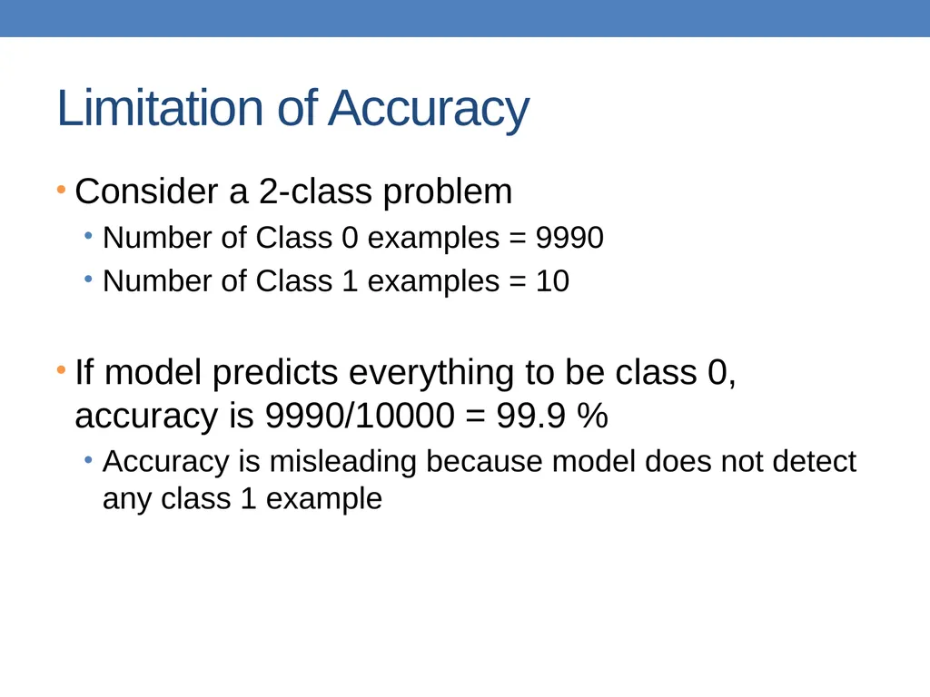
slide70. Limitation of Accuracy Consider a 2-class problem
Number of Class 0 examples = 9990
Number of Class 1 examples = 10
If model predicts everything to be class 0, accuracy is 9990/10000 = 99.9 %
Accuracy is misleading because model does not detect any class 1 example<br>
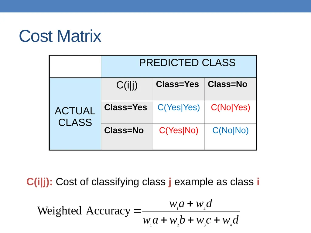
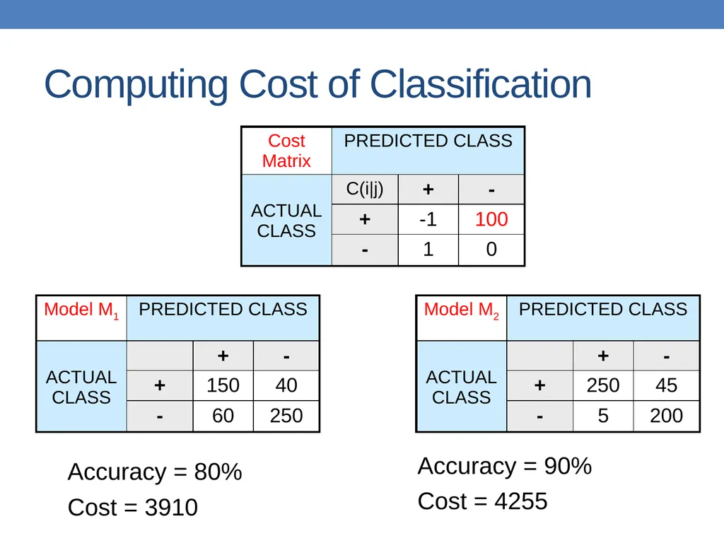
slide71. Cost Matrix C(i|j): Cost of classifying class j example as class i<br>
slide72. Computing Cost of Classification Accuracy = 80%
Cost = 3910 Accuracy = 90%
Cost = 4255<br>
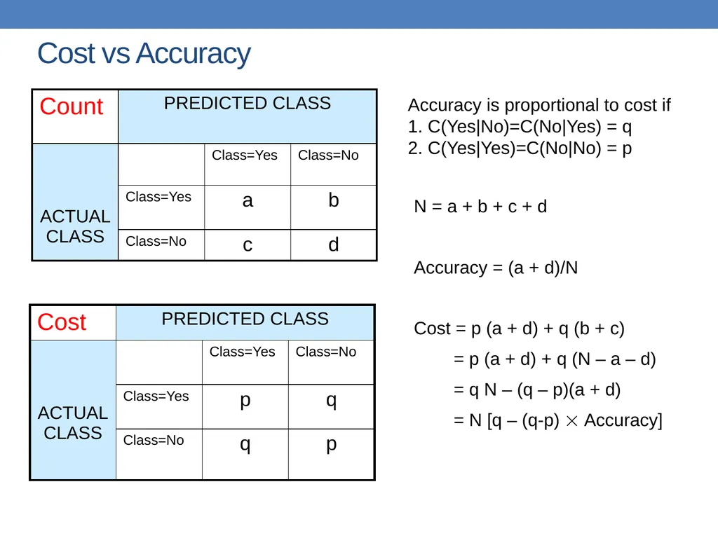
slide73. Cost vs Accuracy<br>
slide74. Precision-Recall Precision is biased towards C(Yes|Yes) & C(Yes|No)
Recall is biased towards C(Yes|Yes) & C(No|Yes)
F-measure is biased towards all except C(No|No)<br>
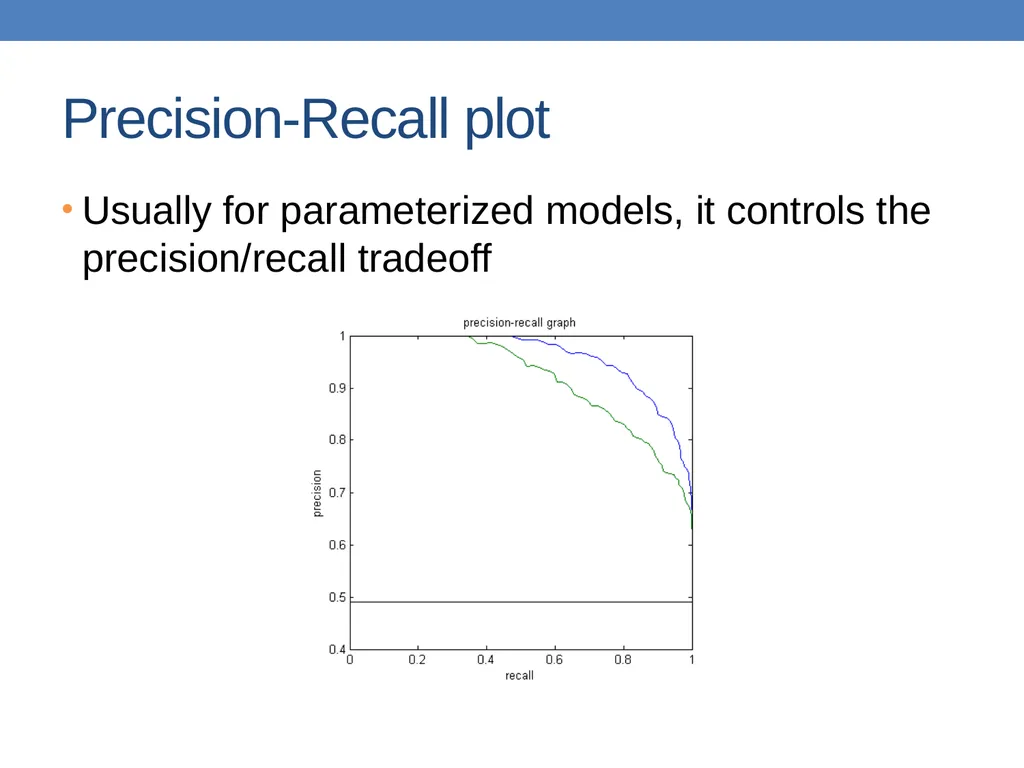
slide75. Precision-Recall plot Usually for parameterized models, it controls the precision/recall tradeoff<br>
slide76. Model Evaluation Metrics for Performance Evaluation
How to evaluate the performance of a model?
Methods for Performance Evaluation
How to obtain reliable estimates?
Methods for Model Comparison
How to compare the relative performance among competing models?<br>
slide77. Methods for Performance Evaluation How to obtain a reliable estimate of performance?
Performance of a model may depend on other factors besides the learning algorithm:
Class distribution
Cost of misclassification
Size of training and test sets<br>
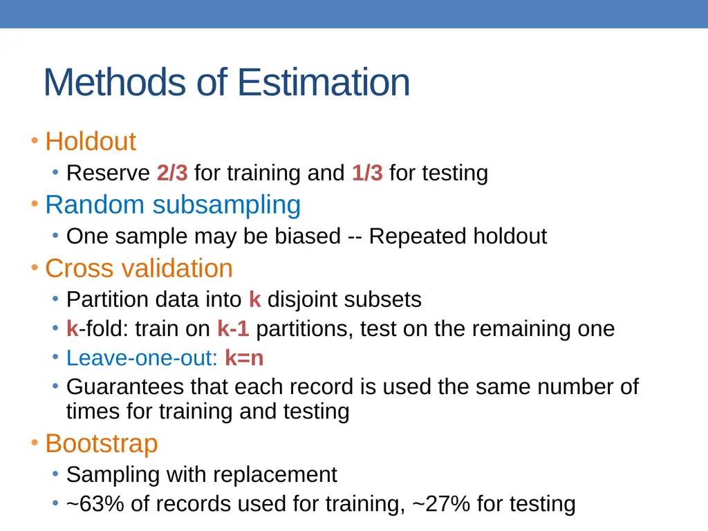
slide78. Methods of Estimation Holdout
Reserve 2/3 for training and 1/3 for testing
Random subsampling
One sample may be biased -- Repeated holdout
Cross validation
Partition data into k disjoint subsets
k-fold: train on k-1 partitions, test on the remaining one
Leave-one-out: k=n
Guarantees that each record is used the same number of times for training and testing
Bootstrap
Sampling with replacement
~63% of records used for training, ~27% for testing<br>
slide79. Dealing with class Imbalance If the class we are interested in is very rare, then the classifier will ignore it.
The class imbalance problem
Solution
We can modify the optimization criterion by using a cost sensitive metric
We can balance the class distribution
Sample from the larger class so that the size of the two classes is the same
Replicate the data of the class of interest so that the classes are balanced
Over-fitting issues<br>
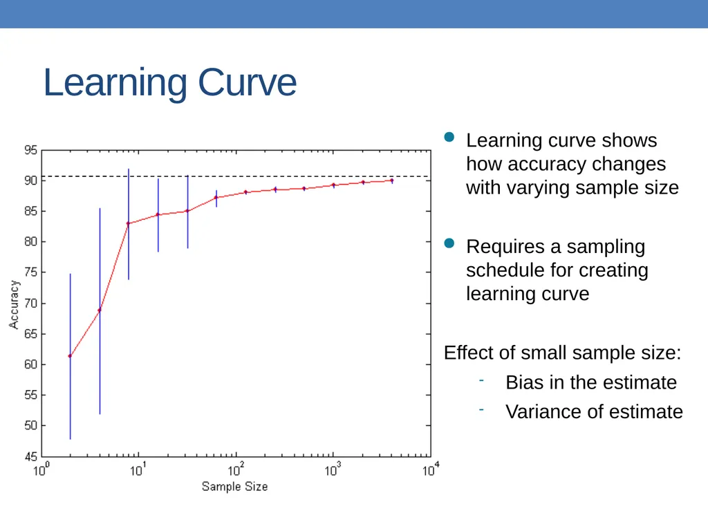
slide80. Learning Curve Learning curve shows how accuracy changes with varying sample size
Requires a sampling schedule for creating learning curve
Effect of small sample size:
Bias in the estimate
Variance of estimate<br>
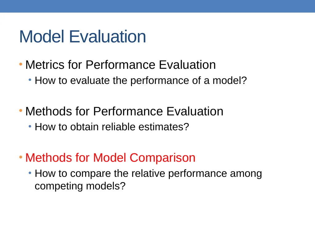
slide81. Model Evaluation Metrics for Performance Evaluation
How to evaluate the performance of a model?
Methods for Performance Evaluation
How to obtain reliable estimates?
Methods for Model Comparison
How to compare the relative performance among competing models?<br>
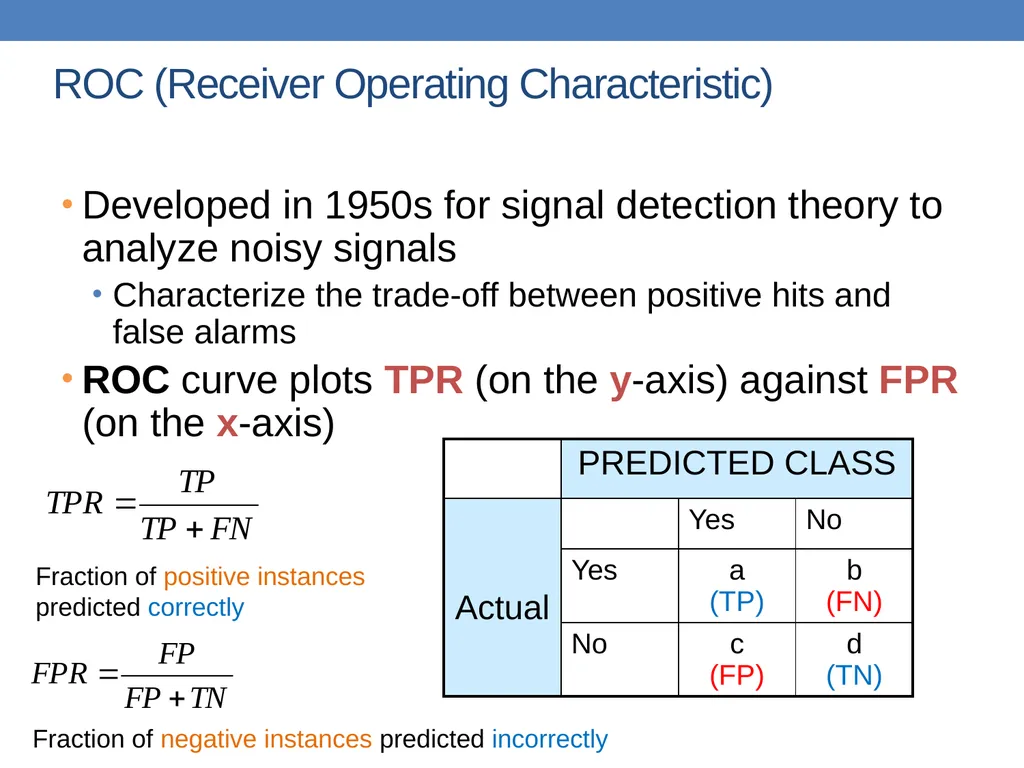
slide82. ROC (Receiver Operating Characteristic) Developed in 1950s for signal detection theory to analyze noisy signals
Characterize the trade-off between positive hits and false alarms
ROC curve plots TPR (on the y-axis) against FPR (on the x-axis) Fraction of positive instances predicted correctly Fraction of negative instances predicted incorrectly<br>
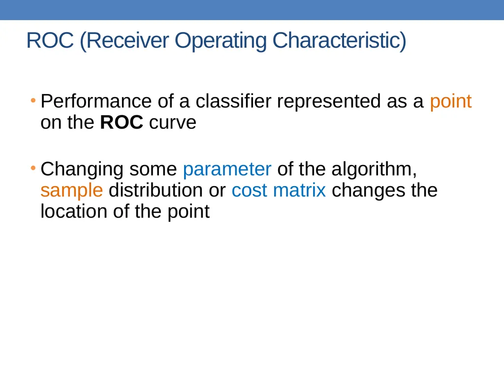
slide83. ROC (Receiver Operating Characteristic) Performance of a classifier represented as a point on the ROC curve
Changing some parameter of the algorithm, sample distribution or cost matrix changes the location of the point<br>
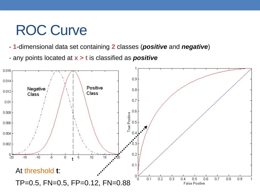
slide84. ROC Curve - 1-dimensional data set containing 2 classes (positive and negative)
- any points located at x > t is classified as positive<br>
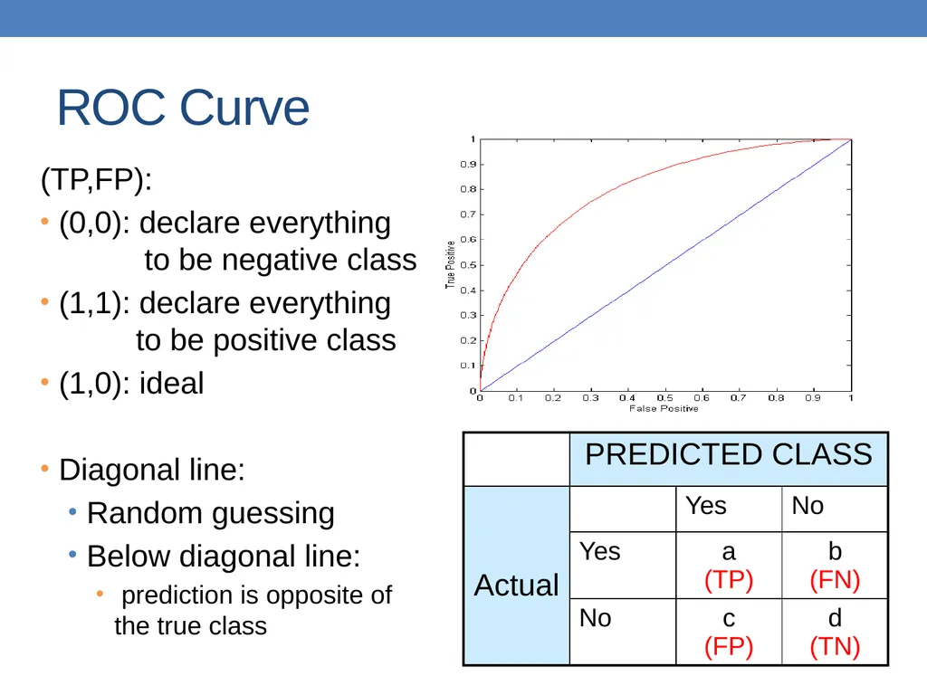
slide85. ROC Curve (TP,FP):
(0,0): declare everything to be negative class
(1,1): declare everything to be positive class
(1,0): ideal
Diagonal line:
Random guessing
Below diagonal line:
prediction is opposite of the true class<br>
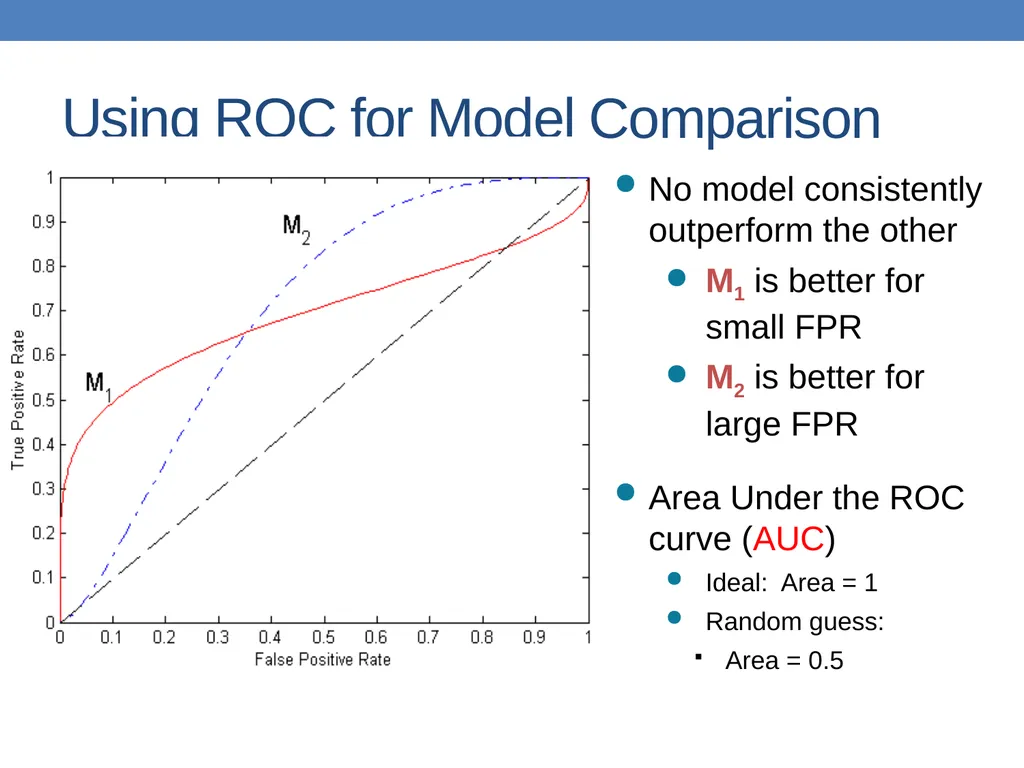
slide86. Using ROC for Model Comparison No model consistently outperform the other
M1 is better for small FPR
M2 is better for large FPR
Area Under the ROC curve (AUC)
Ideal: Area = 1
Random guess:
Area = 0.5<br>
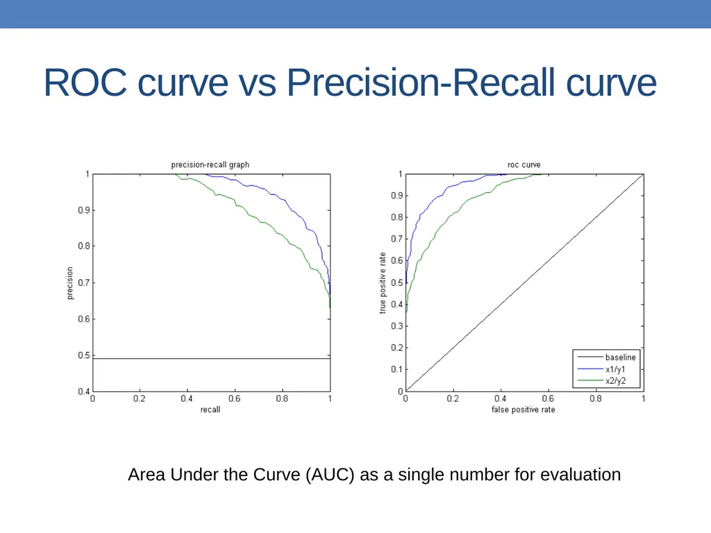
slide87. ROC curve vs Precision-Recall curve Area Under the Curve (AUC) as a single number for evaluation<br>
Basic Concepts
Decision Trees<br>
slide2. Catching tax-evasion Tax-return data for year 2011 A new tax return for 2012
Is this a cheating tax return? An instance of the classification problem: learn a method for discriminating between records of different classes (cheaters vs non-cheaters)<br>
slide3. What is classification? Classification is the task of learning a target function f that maps attribute set x to one of the predefined class labels y One of the attributes is the class attribute
In this case: Cheat
Two class labels (or classes): Yes (1), No (0)<br>
slide4. Why classification? The target function f is known as a classification model
Descriptive modeling: Explanatory tool to distinguish between objects of different classes (e.g., understand why people cheat on their taxes)
Predictive modeling: Predict a class of a previously unseen record<br>
slide5. Examples of Classification Tasks Predicting tumor cells as benign or malignant
Classifying credit card transactions as legitimate or fraudulent
Categorizing news stories as finance, weather, entertainment, sports, etc
Identifying spam email, spam web pages, adult content
Understanding if a web query has commercial intent or not<br>
slide6. General approach to classification Training set consists of records with known class labels
Training set is used to build a classification model
A labeled test set of previously unseen data records is used to evaluate the quality of the model.
The classification model is applied to new records with unknown class labels<br>
slide7. Illustrating Classification Task<br>
slide8. Evaluation of classification models Counts of test records that are correctly (or incorrectly) predicted by the classification model
Confusion matrix Predicted Class Actual Class<br>
slide9. Classification Techniques Decision Tree based Methods
Rule-based Methods
Memory based reasoning
Neural Networks
Naïve Bayes and Bayesian Belief Networks
Support Vector Machines<br>
slide10. Classification Techniques Decision Tree based Methods
Rule-based Methods
Memory based reasoning
Neural Networks
Naïve Bayes and Bayesian Belief Networks
Support Vector Machines<br>
slide11. Decision Trees Decision tree
A flow-chart-like tree structure
Internal node denotes a test on an attribute
Branch represents an outcome of the test
Leaf nodes represent class labels or class distribution<br>
slide12. Example of a Decision Tree Refund MarSt TaxInc YES NO NO NO Yes No Married Single, Divorced < 80K > 80K Splitting Attributes Training Data Model: Decision Tree Test outcome Class labels<br>
slide13. Another Example of Decision Tree categorical categorical continuous class MarSt Refund TaxInc YES NO NO Yes No Married Single, Divorced < 80K > 80K There could be more than one tree that fits the same data!<br>
slide14. Decision Tree Classification Task Decision Tree<br>
slide15. Apply Model to Test Data Test Data Start from the root of tree.<br>
slide16. Apply Model to Test Data Test Data<br>
slide17. Apply Model to Test Data Refund MarSt TaxInc YES NO NO NO Yes No Married Single, Divorced < 80K > 80K Test Data<br>
slide18. Apply Model to Test Data Refund MarSt TaxInc YES NO NO NO Yes No Married Single, Divorced < 80K > 80K Test Data<br>
slide19. Apply Model to Test Data Refund MarSt TaxInc YES NO NO NO Yes No Married Single, Divorced < 80K > 80K Test Data<br>
slide20. Apply Model to Test Data Refund MarSt TaxInc YES NO NO NO Yes No Married Single, Divorced < 80K > 80K Test Data Assign Cheat to “No”<br>
slide21. Decision Tree Classification Task Decision Tree<br>
slide22. Tree Induction Finding the best decision tree is NP-hard
Greedy strategy.
Split the records based on an attribute test that optimizes certain criterion.
Many Algorithms:
Hunt’s Algorithm (one of the earliest)
CART
ID3, C4.5
SLIQ,SPRINT<br>
slide23. General Structure of Hunt’s Algorithm Let Dt be the set of training records that reach a node t
General Procedure:
If Dt contains records that belong the same class yt, then t is a leaf node labeled as yt
If Dt contains records with the same attribute values, then t is a leaf node labeled with the majority class yt
If Dt is an empty set, then t is a leaf node labeled by the default class, yd
If Dt contains records that belong to more than one class, use an attribute test to split the data into smaller subsets.
Recursively apply the procedure to each subset. Dt ?<br>
slide24. Hunt’s Algorithm Don’t
Cheat<br>
slide25. Constructing decision-trees (pseudocode) GenDecTree(Sample S, Features F)
If stopping_condition(S,F) = true then
leaf = createNode()
leaf.label= Classify(S)
return leaf
root = createNode()
root.test_condition = findBestSplit(S,F)
V = {v| v a possible outcome of root.test_condition}
for each value vєV:
Sv: = {s | root.test_condition(s) = v and s є S};
child = GenDecTree(Sv ,F) ;
Add child as a descent of root and label the edge (rootchild) as v
return root<br>
slide26. Tree Induction Issues
How to Classify a leaf node
Assign the majority class
If leaf is empty, assign the default class – the class that has the highest popularity.
Determine how to split the records
How to specify the attribute test condition?
How to determine the best split?
Determine when to stop splitting<br>
slide27. How to Specify Test Condition? Depends on attribute types
Nominal
Ordinal
Continuous
Depends on number of ways to split
2-way split
Multi-way split<br>
slide28. Splitting Based on Nominal Attributes Multi-way split: Use as many partitions as distinct values.
Binary split: Divides values into two subsets. Need to find optimal partitioning. OR<br>
slide29. Multi-way split: Use as many partitions as distinct values.
Binary split: Divides values into two subsets – respects the order. Need to find optimal partitioning.
What about this split? Splitting Based on Ordinal Attributes OR<br>
slide30. Splitting Based on Continuous Attributes Different ways of handling
Discretization to form an ordinal categorical attribute
Static – discretize once at the beginning
Dynamic – ranges can be found by equal interval bucketing, equal frequency bucketing (percentiles), or clustering.
Binary Decision: (A < v) or (A v)
consider all possible splits and finds the best cut
can be more compute intensive<br>
slide31. Splitting Based on Continuous Attributes<br>
slide32. How to determine the Best Split Before Splitting: 10 records of class 0, 10 records of class 1 Which test condition is the best?<br>
slide33. How to determine the Best Split Greedy approach:
Nodes with homogeneous class distribution are preferred
Need a measure of node impurity:
Ideas? Non-homogeneous,
High degree of impurity Homogeneous,
Low degree of impurity<br>
slide34. Measuring Node Impurity p(i|t): fraction of records associated with node t belonging to class i
Used in ID3 and C4.5
Used in CART, SLIQ, SPRINT.<br>
slide35. Gain Gain of an attribute split: compare the impurity of the parent node with the average impurity of the child nodes
Maximizing the gain Minimizing the weighted average impurity measure of children nodes
If I() = Entropy(), then Δinfo is called information gain<br>
slide36. Example P(C1) = 0/6 = 0 P(C2) = 6/6 = 1
Gini = 1 – P(C1)2 – P(C2)2 = 1 – 0 – 1 = 0
Entropy = – 0 log 0 – 1 log 1 = – 0 – 0 = 0
Error = 1 – max (0, 1) = 1 – 1 = 0 P(C1) = 1/6 P(C2) = 5/6
Gini = 1 – (1/6)2 – (5/6)2 = 0.278
Entropy = – (1/6) log2 (1/6) – (5/6) log2 (1/6) = 0.65
Error = 1 – max (1/6, 5/6) = 1 – 5/6 = 1/6 P(C1) = 2/6 P(C2) = 4/6
Gini = 1 – (2/6)2 – (4/6)2 = 0.444
Entropy = – (2/6) log2 (2/6) – (4/6) log2 (4/6) = 0.92
Error = 1 – max (2/6, 4/6) = 1 – 4/6 = 1/3<br>
slide37. Impurity measures All of the impurity measures take value zero (minimum) for the case of a pure node where a single value has probability 1
All of the impurity measures take maximum value when the class distribution in a node is uniform.<br>
slide38. Comparison among Splitting Criteria For a 2-class problem: The different impurity measures are consistent<br>
slide39. Categorical Attributes For binary values split in two
For multivalued attributes, for each distinct value, gather counts for each class in the dataset
Use the count matrix to make decisions Multi-way split Two-way split
(find best partition of values)<br>
slide40. Continuous Attributes Use Binary Decisions based on one value
Choices for the splitting value
Number of possible splitting values = Number of distinct values
Each splitting value has a count matrix associated with it
Class counts in each of the partitions, A < v and A v
Exhaustive method to choose best v
For each v, scan the database to gather count matrix and compute the impurity index
Computationally Inefficient! Repetition of work.<br>
slide41. Continuous Attributes For efficient computation: for each attribute,
Sort the attribute on values
Linearly scan these values, each time updating the count matrix and computing impurity
Choose the split position that has the least impurity<br>
slide42. Splitting based on impurity Impurity measures favor attributes with large number of values
A test condition with large number of outcomes may not be desirable
# of records in each partition is too small to make predictions<br>
slide43. Splitting based on INFO<br>
slide44. Gain Ratio Splitting using information gain
Parent Node, p is split into k partitions
ni is the number of records in partition i
Adjusts Information Gain by the entropy of the partitioning (SplitINFO). Higher entropy partitioning (large number of small partitions) is penalized!
Used in C4.5
Designed to overcome the disadvantage of impurity<br>
slide45. Stopping Criteria for Tree Induction Stop expanding a node when all the records belong to the same class
Stop expanding a node when all the records have similar attribute values
Early termination (to be discussed later)<br>
slide46. Decision Tree Based Classification Advantages:
Inexpensive to construct
Extremely fast at classifying unknown records
Easy to interpret for small-sized trees
Accuracy is comparable to other classification techniques for many simple data sets<br>
slide47. Example: C4.5 Simple depth-first construction.
Uses Information Gain
Sorts Continuous Attributes at each node.
Needs entire data to fit in memory.
Unsuitable for Large Datasets.
Needs out-of-core sorting.
You can download the software from: http://www.cse.unsw.edu.au/~quinlan/c4.5r8.tar.gz<br>
slide48. Other Issues Data Fragmentation
Expressiveness<br>
slide49. Data Fragmentation Number of instances gets smaller as you traverse down the tree
Number of instances at the leaf nodes could be too small to make any statistically significant decision
You can introduce a lower bound on the number of items per leaf node in the stopping criterion.<br>
slide50. Expressiveness A classifier defines a function that discriminates between two (or more) classes.
The expressiveness of a classifier is the class of functions that it can model, and the kind of data that it can separate
When we have discrete (or binary) values, we are interested in the class of boolean functions that can be modeled
If the data-points are real vectors we talk about the decision boundary that the classifier can model<br>
slide51. Decision Boundary Border line between two neighboring regions of different classes is known as decision boundary
Decision boundary is parallel to axes because test condition involves a single attribute at-a-time<br>
slide52. Expressiveness Decision tree provides expressive representation for learning discrete-valued function
But they do not generalize well to certain types of Boolean functions
Example: parity function:
Class = 1 if there is an even number of Boolean attributes with truth value = True
Class = 0 if there is an odd number of Boolean attributes with truth value = True
For accurate modeling, must have a complete tree
Less expressive for modeling continuous variables
Particularly when test condition involves only a single attribute at-a-time<br>
slide53. Oblique Decision Trees Test condition may involve multiple attributes
More expressive representation
Finding optimal test condition is computationally expensive<br>
slide54. Practical Issues of Classification Underfitting and Overfitting
Evaluation<br>
slide55. Underfitting and Overfitting (Example) 500 circular and 500 triangular data points.
Circular points:
0.5 sqrt(x12+x22) 1
Triangular points:
sqrt(x12+x22) > 0.5 or
sqrt(x12+x22) < 1<br>
slide56. Underfitting and Overfitting Overfitting Underfitting: when model is too simple, both training and test errors are large Underfitting Overfitting: when model is too complex it models the details of the training set and fails on the test set<br>
slide57. Overfitting due to Noise Decision boundary is distorted by noise point<br>
slide58. Overfitting due to Insufficient Examples Lack of data points in the lower half of the diagram makes it difficult to predict correctly the class labels of that region
- Insufficient number of training records in the region causes the decision tree to predict the test examples using other training records that are irrelevant to the classification task<br>
slide59. Notes on Overfitting Overfitting results in decision trees that are more complex than necessary
Training error no longer provides a good estimate of how well the tree will perform on previously unseen records
The model does not generalize well
Need new ways for estimating errors<br>
slide60. Estimating Generalization Errors<br>
slide61. Occam’s Razor Given two models of similar generalization errors, one should prefer the simpler model over the more complex model
For complex models, there is a greater chance that it was fitted accidentally by errors in data
Therefore, one should include model complexity when evaluating a model<br>
slide62. Minimum Description Length (MDL) Cost(Model,Data) = Cost(Data|Model) + Cost(Model)
Search for the least costly model.
Cost(Data|Model) encodes the misclassification errors.
Cost(Model) encodes the decision tree
node encoding (number of children) plus splitting condition encoding.<br>
slide63. How to Address Overfitting Pre-Pruning (Early Stopping Rule)
Stop the algorithm before it becomes a fully-grown tree
Typical stopping conditions for a node:
Stop if all instances belong to the same class
Stop if all the attribute values are the same
More restrictive conditions:
Stop if number of instances is less than some user-specified threshold
Stop if class distribution of instances are independent of the available features (e.g., using 2 test)
Stop if expanding the current node does not improve impurity measures (e.g., Gini or information gain).<br>
slide64. How to Address Overfitting… Post-pruning
Grow decision tree to its entirety
Trim the nodes of the decision tree in a bottom-up fashion
If generalization error improves after trimming, replace sub-tree by a leaf node.
Class label of leaf node is determined from majority class of instances in the sub-tree
Can use MDL for post-pruning<br>
slide65. Example of Post-Pruning Training Error (Before splitting) = 10/30
Pessimistic error = (10 + 0.5)/30 = 10.5/30
Training Error (After splitting) = 9/30
Pessimistic error (After splitting)
= (9 + 4 0.5)/30 = 11/30
PRUNE!<br>
slide66. Model Evaluation Metrics for Performance Evaluation
How to evaluate the performance of a model?
Methods for Performance Evaluation
How to obtain reliable estimates?
Methods for Model Comparison
How to compare the relative performance among competing models?<br>
slide67. Model Evaluation Metrics for Performance Evaluation
How to evaluate the performance of a model?
Methods for Performance Evaluation
How to obtain reliable estimates?
Methods for Model Comparison
How to compare the relative performance among competing models?<br>
slide68. Metrics for Performance Evaluation Focus on the predictive capability of a model
Rather than how fast it takes to classify or build models, scalability, etc.
Confusion Matrix: a: TP (true positive)
b: FN (false negative)
c: FP (false positive)
d: TN (true negative)<br>
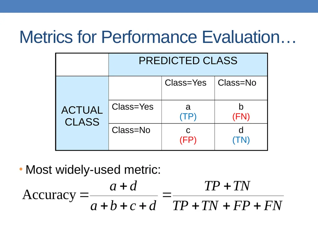
slide69. Metrics for Performance Evaluation… Most widely-used metric:<br>
slide70. Limitation of Accuracy Consider a 2-class problem
Number of Class 0 examples = 9990
Number of Class 1 examples = 10
If model predicts everything to be class 0, accuracy is 9990/10000 = 99.9 %
Accuracy is misleading because model does not detect any class 1 example<br>
slide71. Cost Matrix C(i|j): Cost of classifying class j example as class i<br>
slide72. Computing Cost of Classification Accuracy = 80%
Cost = 3910 Accuracy = 90%
Cost = 4255<br>
slide73. Cost vs Accuracy<br>
slide74. Precision-Recall Precision is biased towards C(Yes|Yes) & C(Yes|No)
Recall is biased towards C(Yes|Yes) & C(No|Yes)
F-measure is biased towards all except C(No|No)<br>
slide75. Precision-Recall plot Usually for parameterized models, it controls the precision/recall tradeoff<br>
slide76. Model Evaluation Metrics for Performance Evaluation
How to evaluate the performance of a model?
Methods for Performance Evaluation
How to obtain reliable estimates?
Methods for Model Comparison
How to compare the relative performance among competing models?<br>
slide77. Methods for Performance Evaluation How to obtain a reliable estimate of performance?
Performance of a model may depend on other factors besides the learning algorithm:
Class distribution
Cost of misclassification
Size of training and test sets<br>
slide78. Methods of Estimation Holdout
Reserve 2/3 for training and 1/3 for testing
Random subsampling
One sample may be biased -- Repeated holdout
Cross validation
Partition data into k disjoint subsets
k-fold: train on k-1 partitions, test on the remaining one
Leave-one-out: k=n
Guarantees that each record is used the same number of times for training and testing
Bootstrap
Sampling with replacement
~63% of records used for training, ~27% for testing<br>
slide79. Dealing with class Imbalance If the class we are interested in is very rare, then the classifier will ignore it.
The class imbalance problem
Solution
We can modify the optimization criterion by using a cost sensitive metric
We can balance the class distribution
Sample from the larger class so that the size of the two classes is the same
Replicate the data of the class of interest so that the classes are balanced
Over-fitting issues<br>
slide80. Learning Curve Learning curve shows how accuracy changes with varying sample size
Requires a sampling schedule for creating learning curve
Effect of small sample size:
Bias in the estimate
Variance of estimate<br>
slide81. Model Evaluation Metrics for Performance Evaluation
How to evaluate the performance of a model?
Methods for Performance Evaluation
How to obtain reliable estimates?
Methods for Model Comparison
How to compare the relative performance among competing models?<br>
slide82. ROC (Receiver Operating Characteristic) Developed in 1950s for signal detection theory to analyze noisy signals
Characterize the trade-off between positive hits and false alarms
ROC curve plots TPR (on the y-axis) against FPR (on the x-axis) Fraction of positive instances predicted correctly Fraction of negative instances predicted incorrectly<br>
slide83. ROC (Receiver Operating Characteristic) Performance of a classifier represented as a point on the ROC curve
Changing some parameter of the algorithm, sample distribution or cost matrix changes the location of the point<br>
slide84. ROC Curve - 1-dimensional data set containing 2 classes (positive and negative)
- any points located at x > t is classified as positive<br>
slide85. ROC Curve (TP,FP):
(0,0): declare everything to be negative class
(1,1): declare everything to be positive class
(1,0): ideal
Diagonal line:
Random guessing
Below diagonal line:
prediction is opposite of the true class<br>
slide86. Using ROC for Model Comparison No model consistently outperform the other
M1 is better for small FPR
M2 is better for large FPR
Area Under the ROC curve (AUC)
Ideal: Area = 1
Random guess:
Area = 0.5<br>
slide87. ROC curve vs Precision-Recall curve Area Under the Curve (AUC) as a single number for evaluation<br>