Deep Learning for Natural Language Processing DLNLP 10: Recurrent Neural Networks Mihai Surdeanu and Marco A. Valenzuela-Escarcega 1 Overview Vanilla recurrent neural networks (RNN) Deep RNNs Long short-term memory networks (LSTM)
"Deep Learning for Natural Language Processing" is the property of its rightful owner. Permission is granted to
download and print the materials on this website for personal, non-commercial use only, and to display it
on your personal computer provided you do not modify the materials and that you retain all copyright
notices contained in the materials. By downloading content from our website, you accept the terms of this
agreement.
Presentation Transcript
01
Deep Learning for Natural Language Processing DLNLP 10: Recurrent Neural Networks Mihai Surdeanu and Marco A. Valenzuela-Escárcega 1<br>
02
Overview Vanilla recurrent neural networks (RNN)
Deep RNNs
Long short-term memory networks (LSTM)
Conditional random fields
Drawbacks 2<br>
03
Bag-of-words methods Up to this point, we have only discussed neural approaches for text classification (e.g., review and news classification) that handle the text as a bag of words.
These methods are very effective! 3<br>
04
Word order is important For many NLP tasks, we need to capture the word-order information more explicitly.
What are examples of such applications?
In this chapter, we will discuss one direction for explicitly modeling word order: recurrent neural networks (RNN).
Starting with chapter 14, we will discuss transformer networks. 4<br>
05
Vanilla rnns 5<br>
06
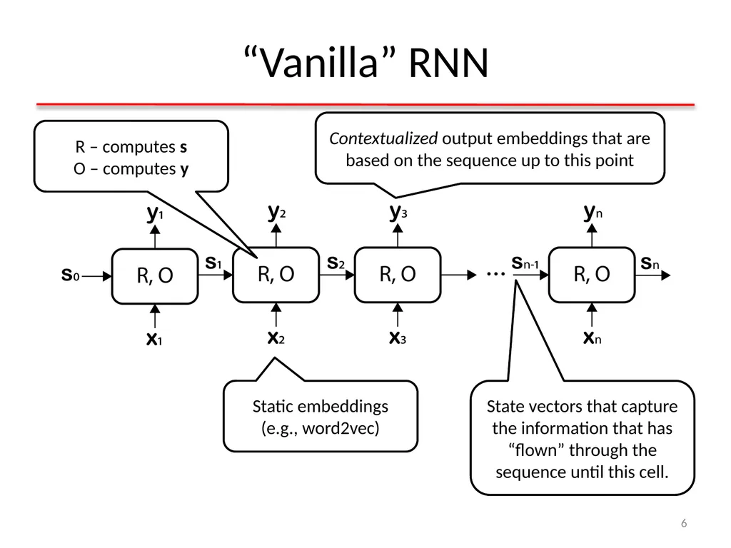
“Vanilla” RNN 6 Static embeddings (e.g., word2vec) Contextualized output embeddings that are based on the sequence up to this point State vectors that capture the information that has “flown” through the sequence until this cell. R – computes s
O – computes y<br>
07
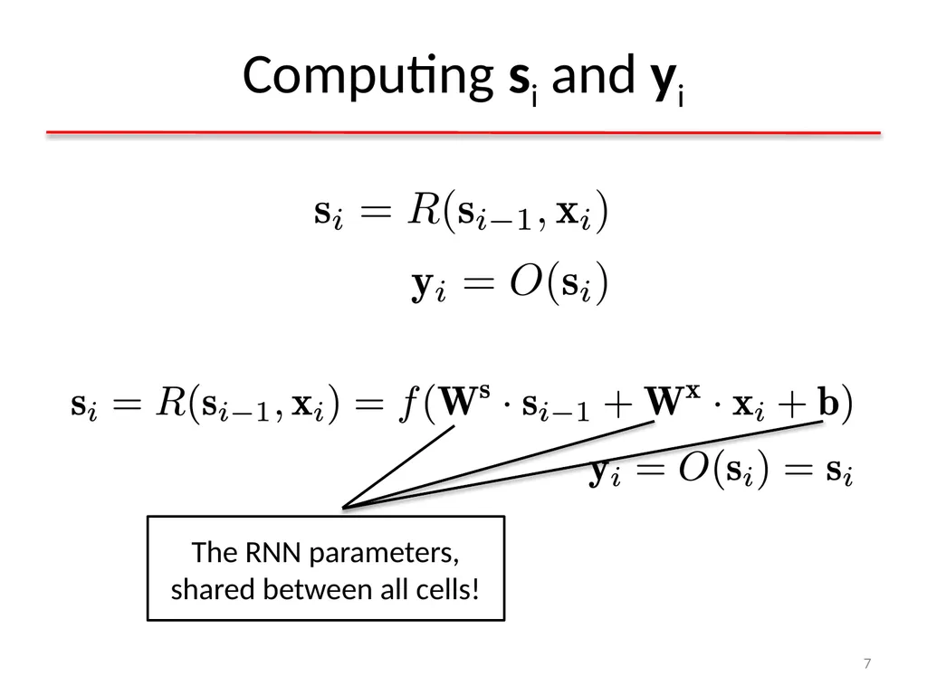
Computing si and yi 7<br>
08
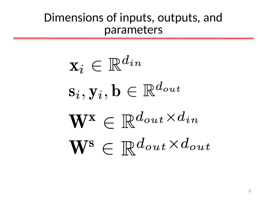
Dimensions of inputs, outputs, and parameters 8<br>
09
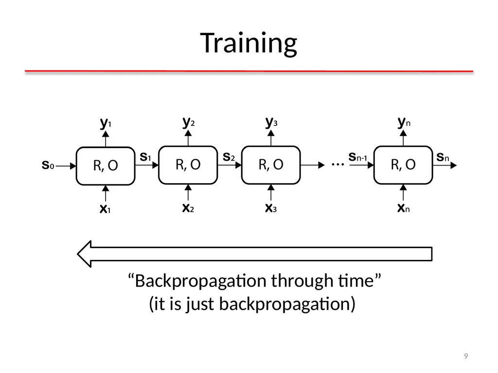
Training 9 “Backpropagation through time”
(it is just backpropagation)<br>
10
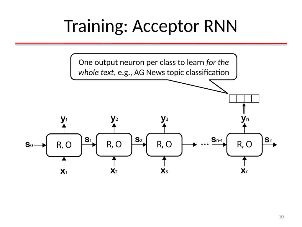
Training: Acceptor RNN 10 One output neuron per class to learn for the whole text, e.g., AG News topic classification<br>
11
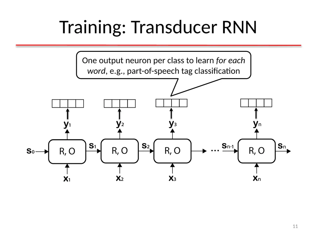
Training: Transducer RNN 11 One output neuron per class to learn for each word, e.g., part-of-speech tag classification<br>
12
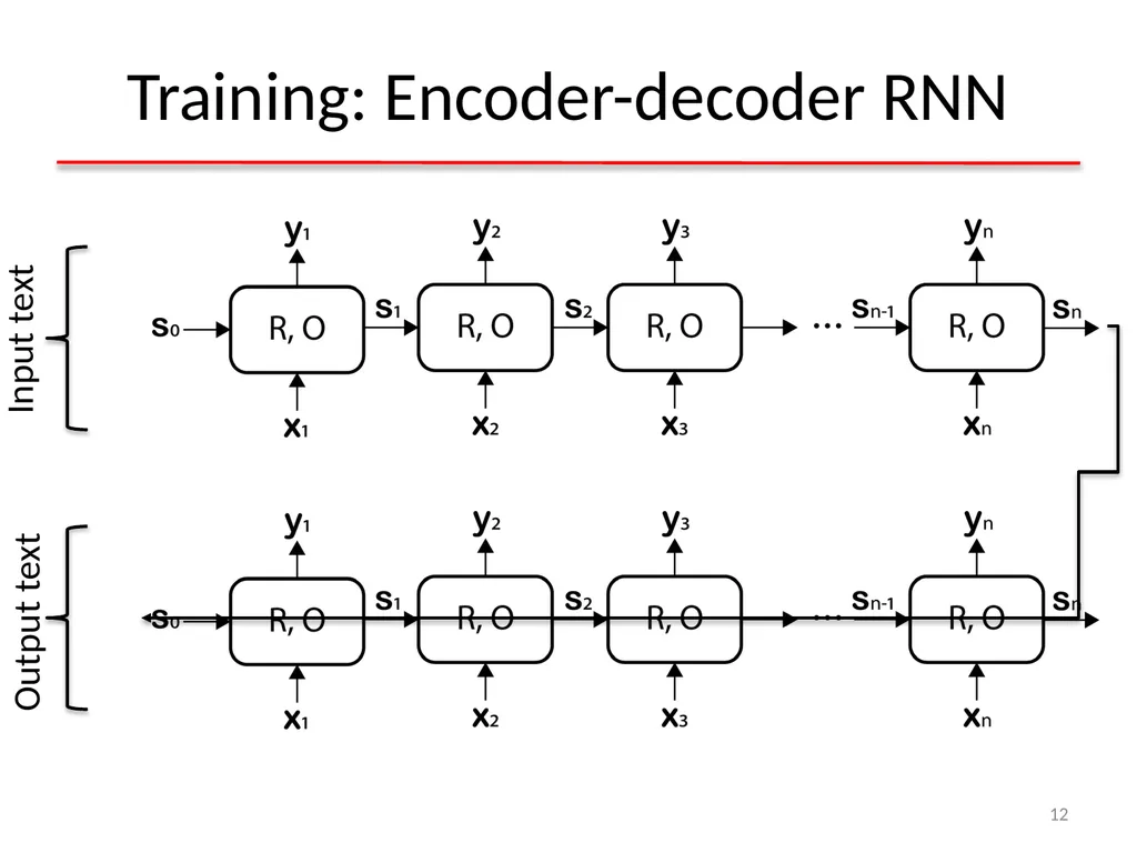
Training: Encoder-decoder RNN 12<br>
13
deep rnns 13<br>
14
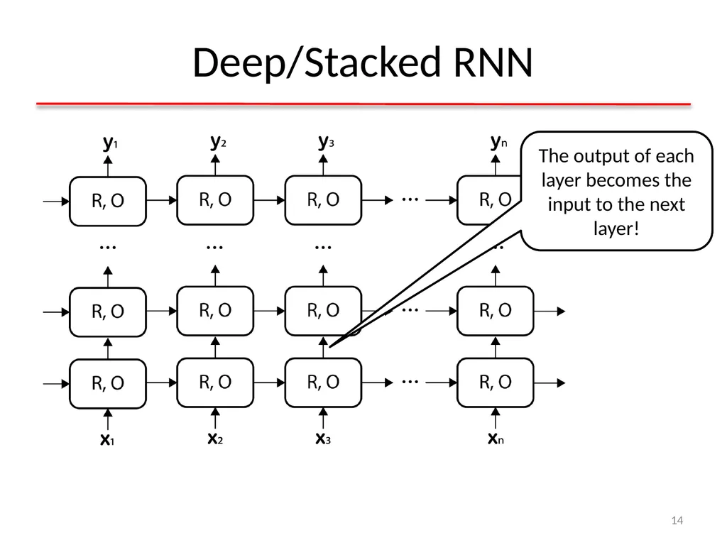
Deep/Stacked RNN 14 The output of each layer becomes the input to the next layer!<br>
15
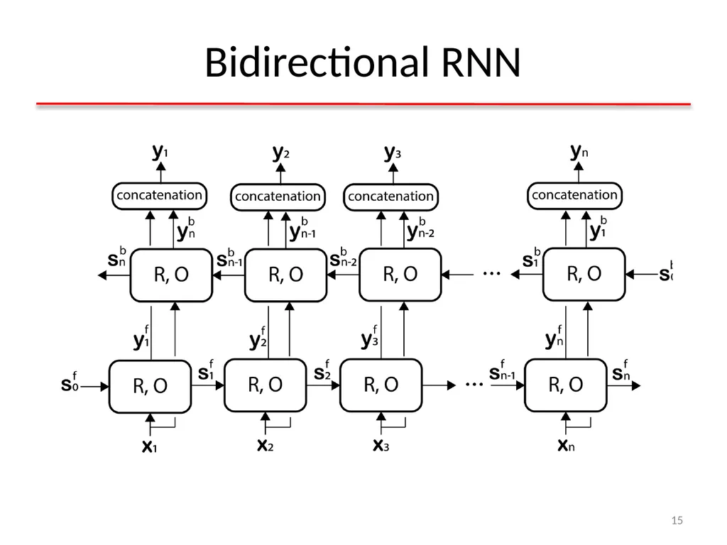
Bidirectional RNN 15<br>
16
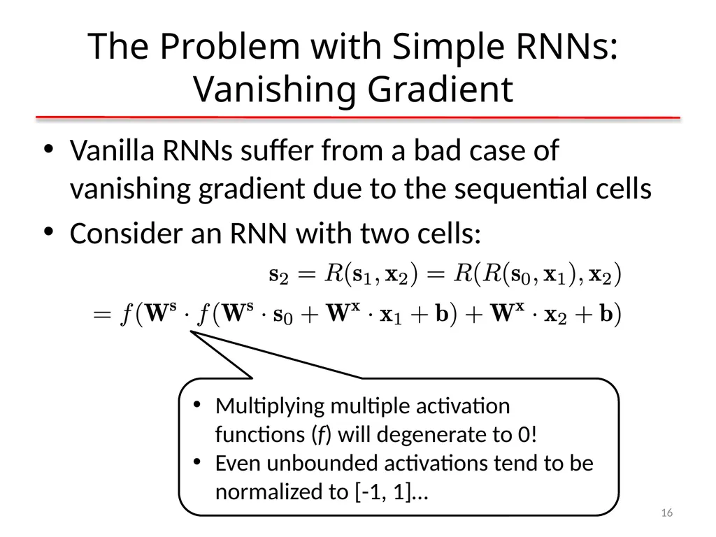
The Problem with Simple RNNs: Vanishing Gradient Vanilla RNNs suffer from a bad case of vanishing gradient due to the sequential cells
Consider an RNN with two cells: 16 Multiplying multiple activation functions (f) will degenerate to 0!
Even unbounded activations tend to be normalized to [-1, 1]…<br>
17
Long short-memory networks 17<br>
18
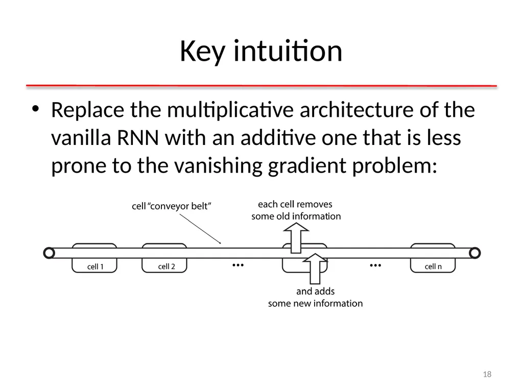
Key intuition Replace the multiplicative architecture of the vanilla RNN with an additive one that is less prone to the vanishing gradient problem: 18<br>
19
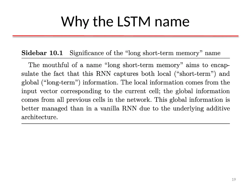
Why the LSTM name 19<br>
20
LSTM building block: the neural gate 20 Binary gate Gate with real-valued elements<br>
21
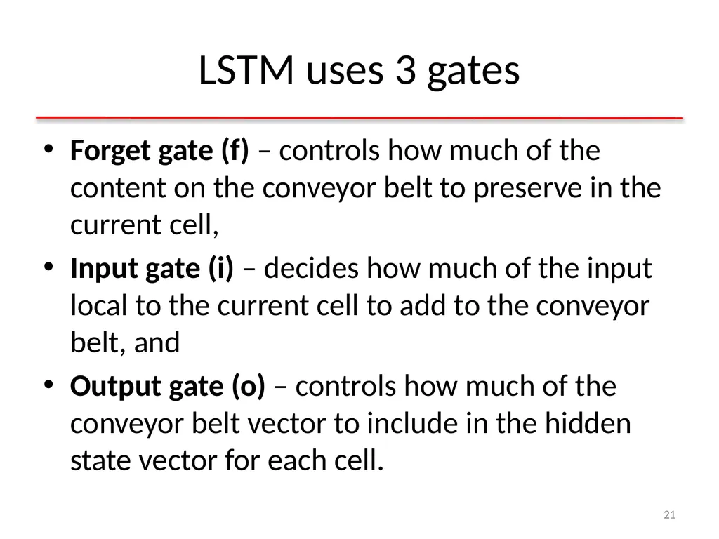
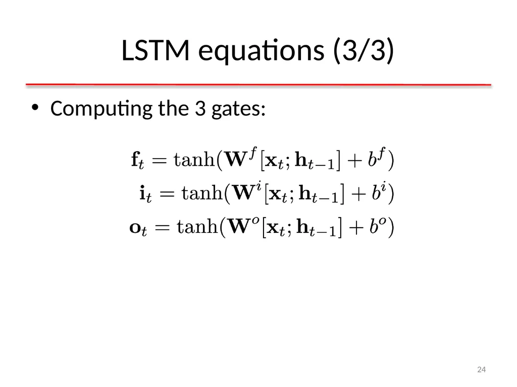
LSTM uses 3 gates Forget gate (f) – controls how much of the content on the conveyor belt to preserve in the current cell,
Input gate (i) – decides how much of the input local to the current cell to add to the conveyor belt, and
Output gate (o) – controls how much of the conveyor belt vector to include in the hidden state vector for each cell. 21<br>
22
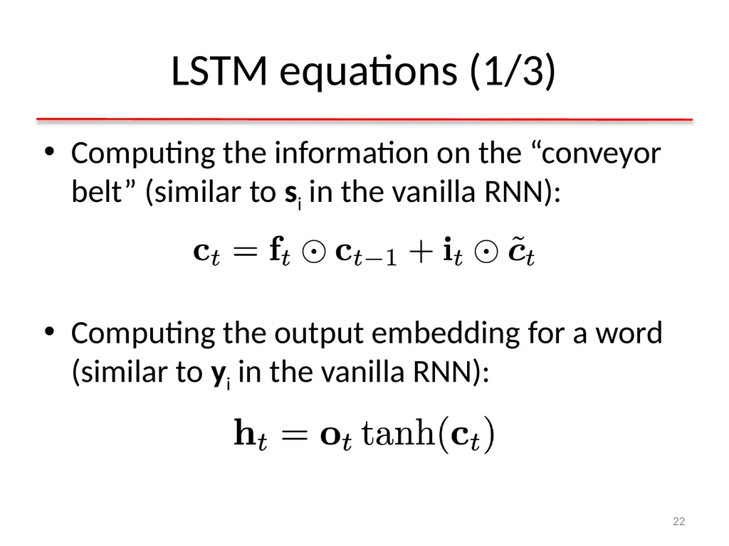
LSTM equations (1/3) Computing the information on the “conveyor belt” (similar to si in the vanilla RNN):
Computing the output embedding for a word (similar to yi in the vanilla RNN): 22<br>
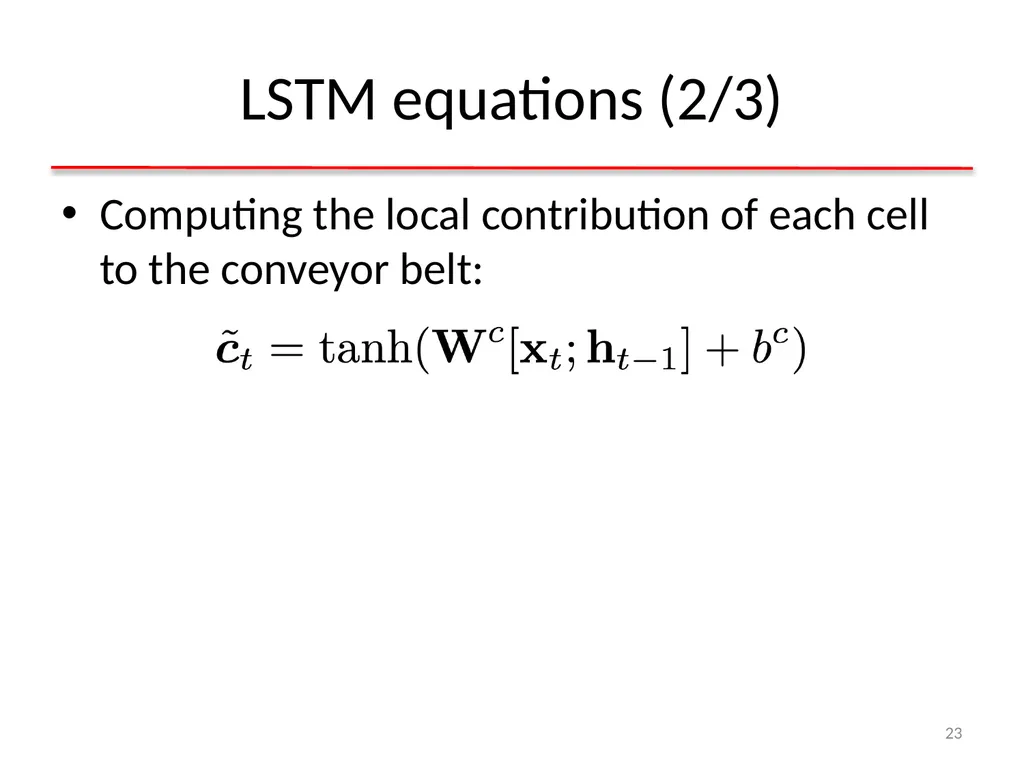
23
LSTM equations (2/3) Computing the local contribution of each cell to the conveyor belt: 23<br>
24
LSTM equations (3/3) Computing the 3 gates: 24<br>
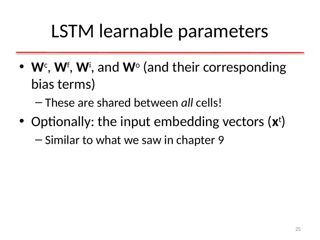
25
LSTM learnable parameters Wc, Wf, Wi, and Wo (and their corresponding bias terms)
These are shared between all cells!
Optionally: the input embedding vectors (xt)
Similar to what we saw in chapter 9 25<br>
26
Vanishing vs. exploding gradients Additive architectures such as the LSTM mitigate the vanishing gradient problem
But they suffer from the exploding gradient problem, i.e., when gradient values become very large in magnitude. Why?
Exploding gradients is a serious problem because it leads to unstable training.
Solutions:
Everything we discussed in chapter 6, i.e., small learning rates, Xavier initialization, output normalization
In addition: gradient clipping. 26<br>
27
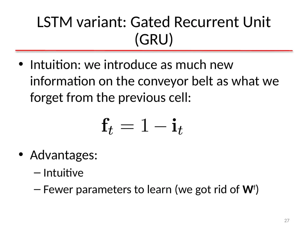
LSTM variant: Gated Recurrent Unit (GRU) Intuition: we introduce as much new information on the conveyor belt as what we forget from the previous cell:
Advantages:
Intuitive
Fewer parameters to learn (we got rid of Wf) 27<br>
28
LSTM advantages/disadvantages Advantages
Additive recurrent architectures are (more) resistant to vanishing gradient
Fundamental for many applications that depend on sequences
Disadvantages
“Fuzzy far away” (Khandelwal et al., 2018)
Hard to parallelize
Exploding gradient
More explanations and visualizations: https://colah.github.io/posts/2015-08-Understanding-LSTMs/ 28<br>
29
Take away Vanilla recurrent neural networks (RNN)
Deep RNNs
Long short-term memory networks (LSTM)
Conditional random fields
Drawbacks 29<br>