04
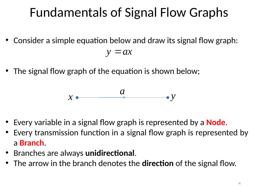
Fundamentals of Signal Flow Graphs Consider a simple equation below and draw its signal flow graph:
The signal flow graph of the equation is shown below;
Every variable in a signal flow graph is represented by a Node.
Every transmission function in a signal flow graph is represented by a Branch.
Branches are always unidirectional.
The arrow in the branch denotes the direction of the signal flow. 4<br>
05
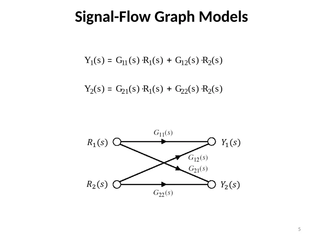
Signal-Flow Graph Models 5<br>
06
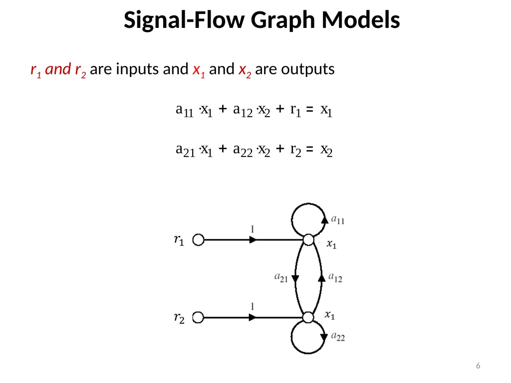
Signal-Flow Graph Models r1 and r2 are inputs and x1 and x2 are outputs 6<br>
07
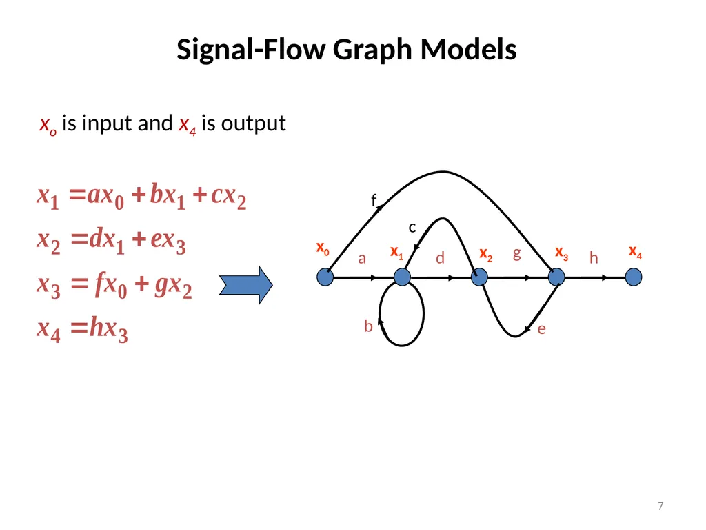
Signal-Flow Graph Models xo is input and x4 is output 7<br>
08
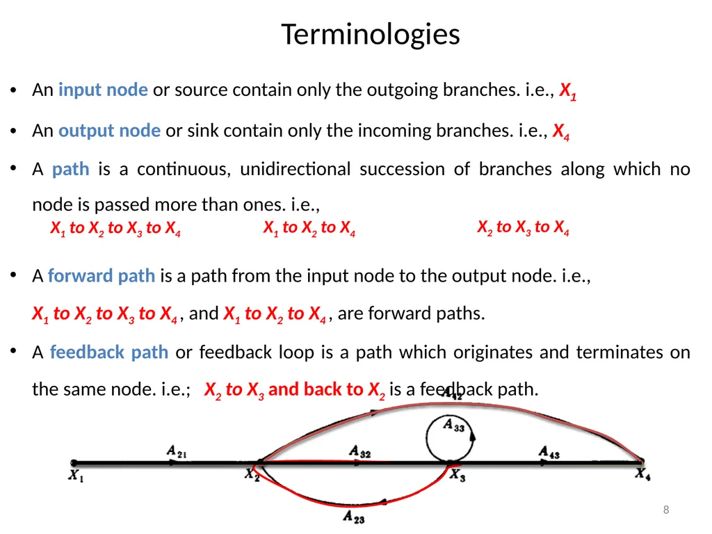
Terminologies An input node or source contain only the outgoing branches. i.e., X1
An output node or sink contain only the incoming branches. i.e., X4
A path is a continuous, unidirectional succession of branches along which no node is passed more than ones. i.e.,
A forward path is a path from the input node to the output node. i.e.,
X1 to X2 to X3 to X4 , and X1 to X2 to X4 , are forward paths.
A feedback path or feedback loop is a path which originates and terminates on the same node. i.e.; X2 to X3 and back to X2 is a feedback path. 8<br>
09
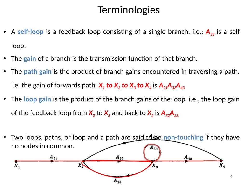
Terminologies A self-loop is a feedback loop consisting of a single branch. i.e.; A33 is a self loop.
The gain of a branch is the transmission function of that branch.
The path gain is the product of branch gains encountered in traversing a path. i.e. the gain of forwards path X1 to X2 to X3 to X4 is A21A32A43
The loop gain is the product of the branch gains of the loop. i.e., the loop gain of the feedback loop from X2 to X3 and back to X2 is A32A23.
Two loops, paths, or loop and a path are said to be non-touching if they have no nodes in common. 9<br>
10
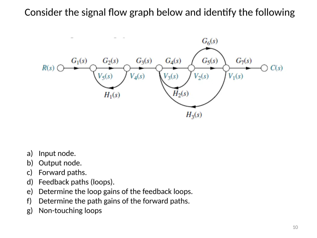
Consider the signal flow graph below and identify the following Input node.
Output node.
Forward paths.
Feedback paths (loops).
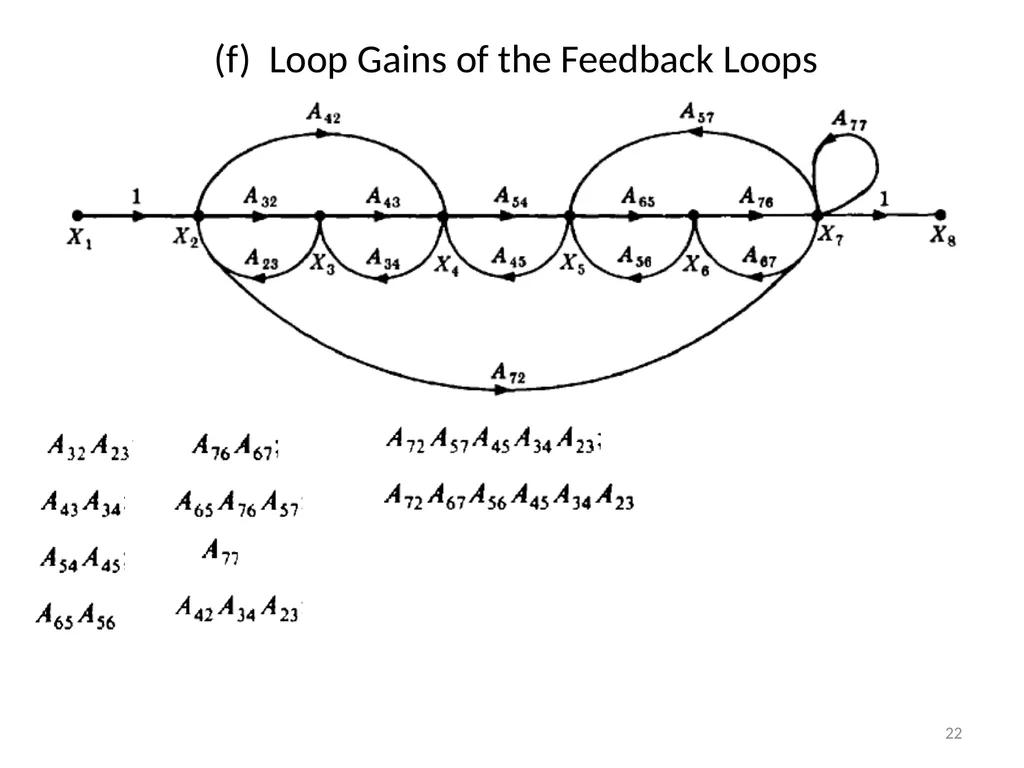
Determine the loop gains of the feedback loops.
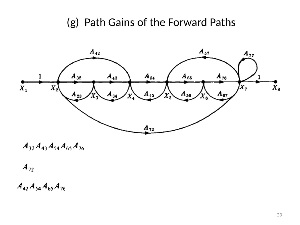
Determine the path gains of the forward paths.
Non-touching loops 10<br>
11
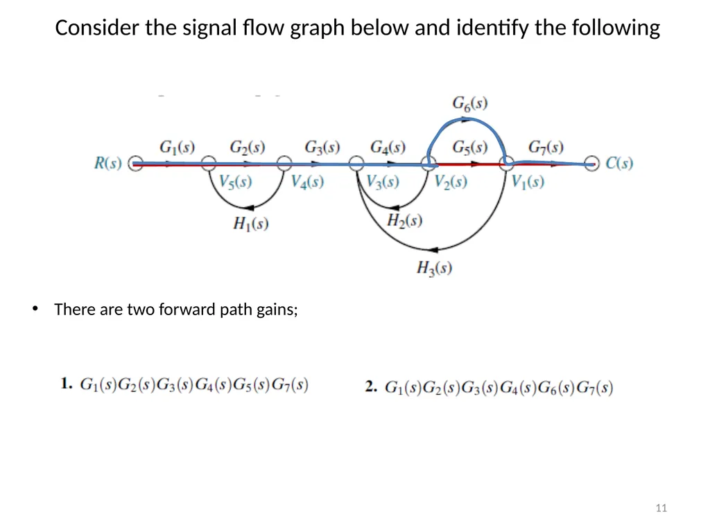
Consider the signal flow graph below and identify the following There are two forward path gains; 11<br>
12
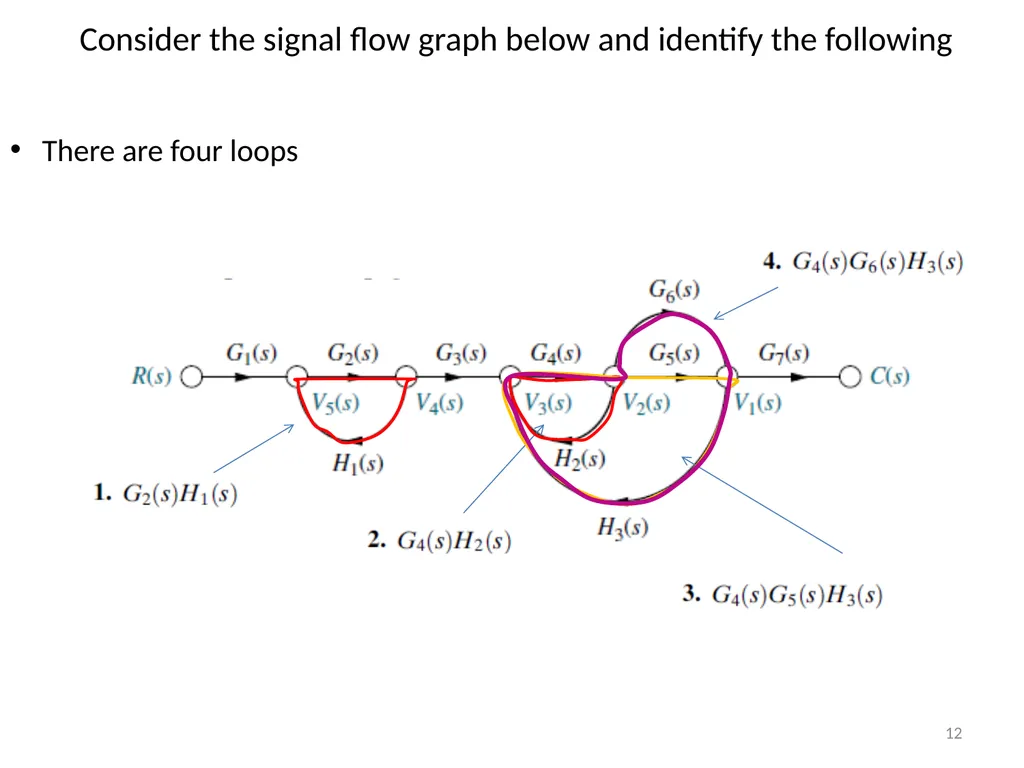
Consider the signal flow graph below and identify the following There are four loops 12<br>
13
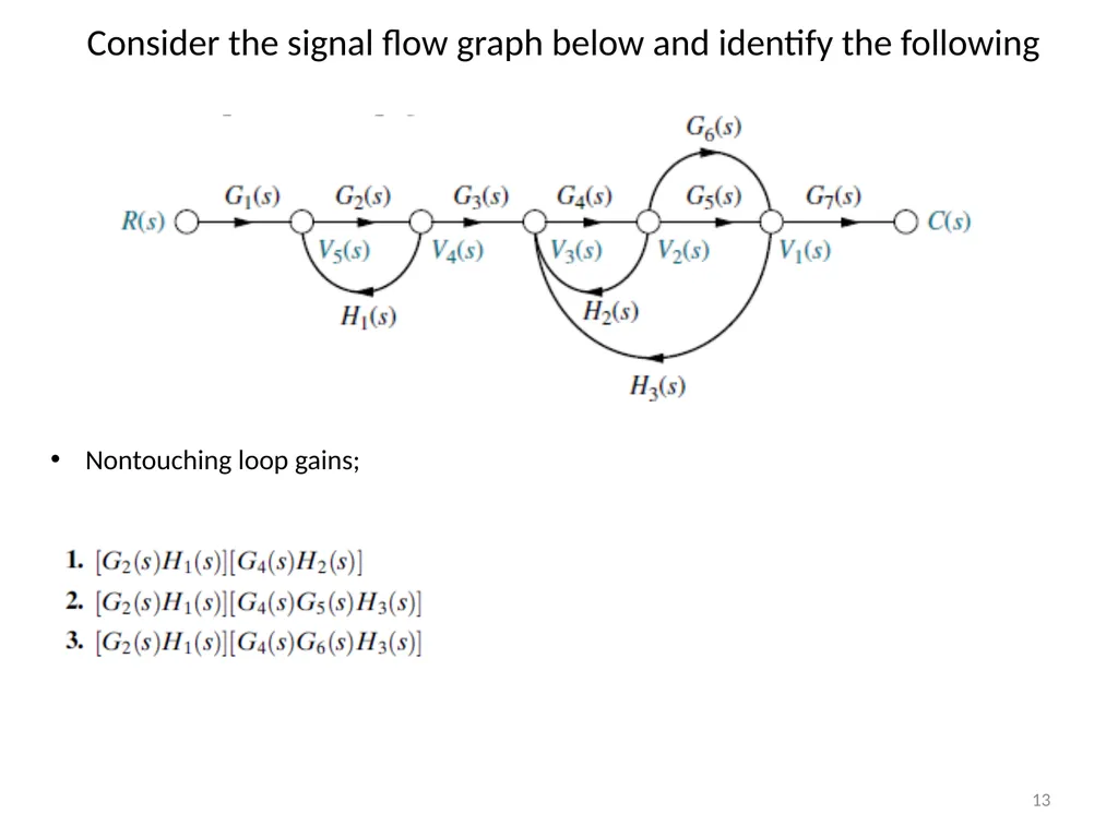
Consider the signal flow graph below and identify the following Nontouching loop gains; 13<br>
14
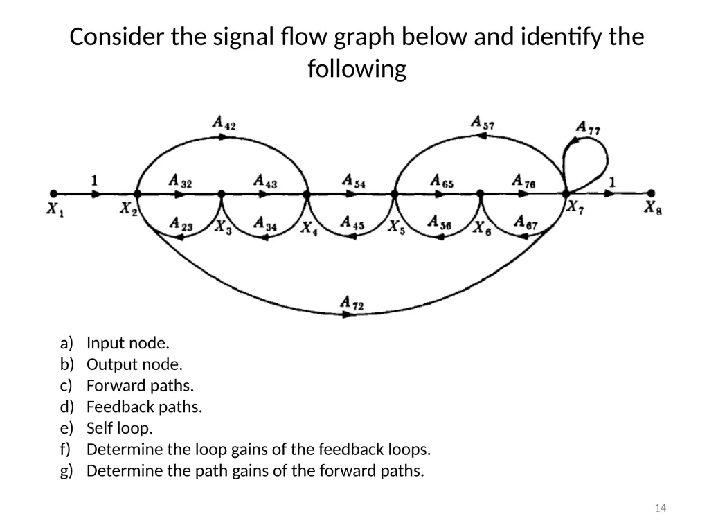
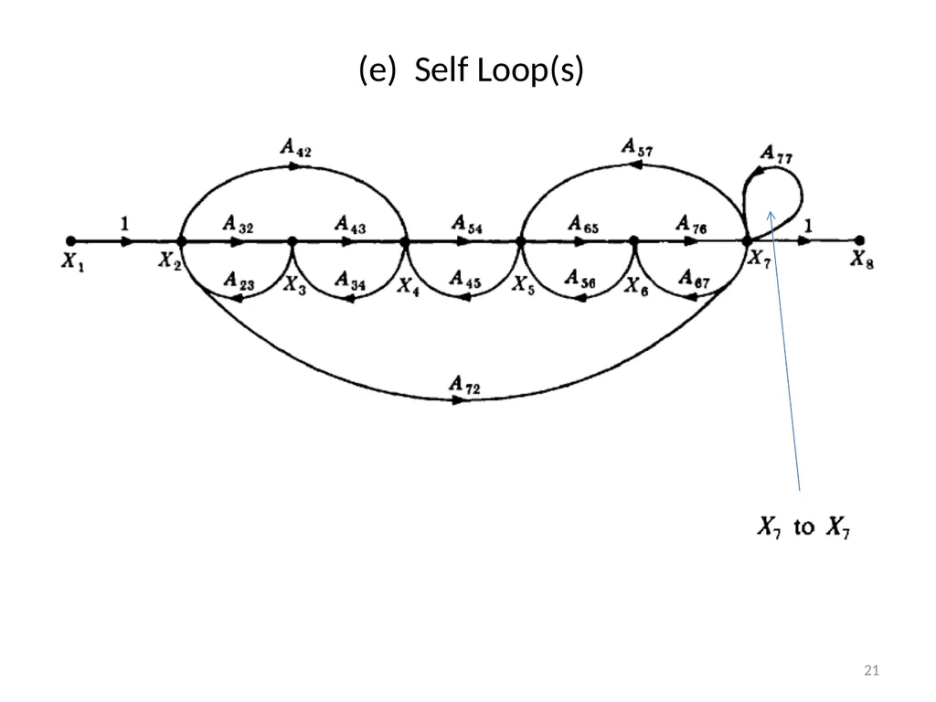
Consider the signal flow graph below and identify the following Input node.
Output node.
Forward paths.
Feedback paths.
Self loop.
Determine the loop gains of the feedback loops.
Determine the path gains of the forward paths. 14<br>
15
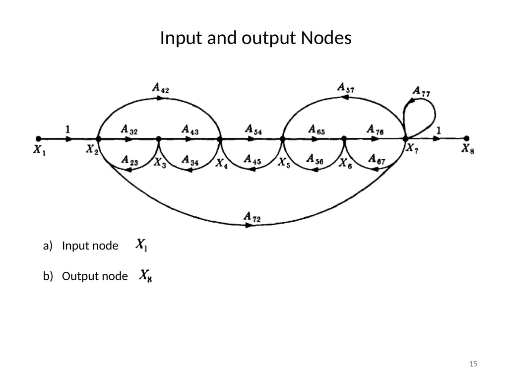
Input and output Nodes Input node
Output node 15<br>
16
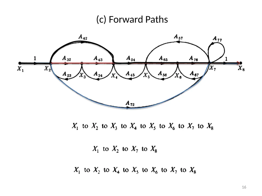
(c) Forward Paths 16<br>
17
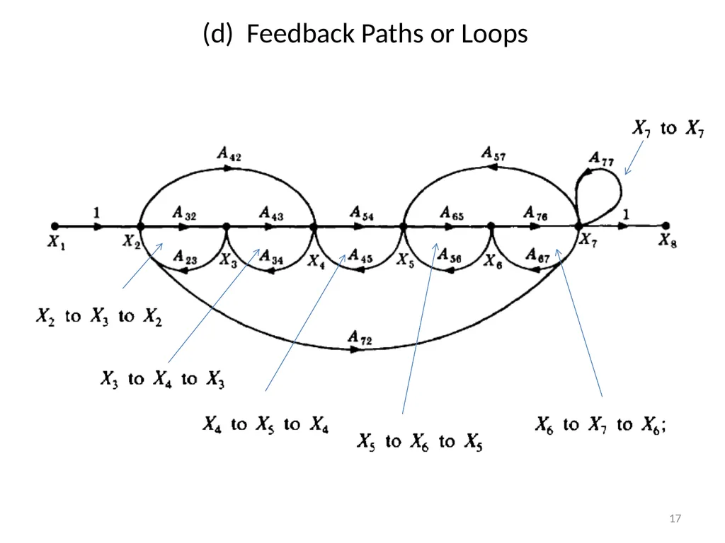
(d) Feedback Paths or Loops 17<br>
18
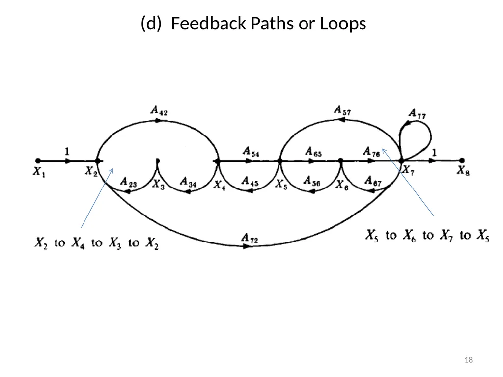
(d) Feedback Paths or Loops 18<br>
19
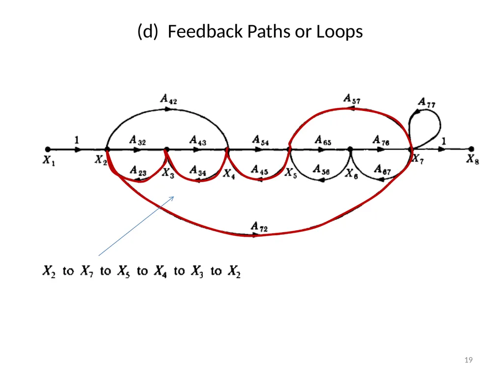
(d) Feedback Paths or Loops 19<br>
20
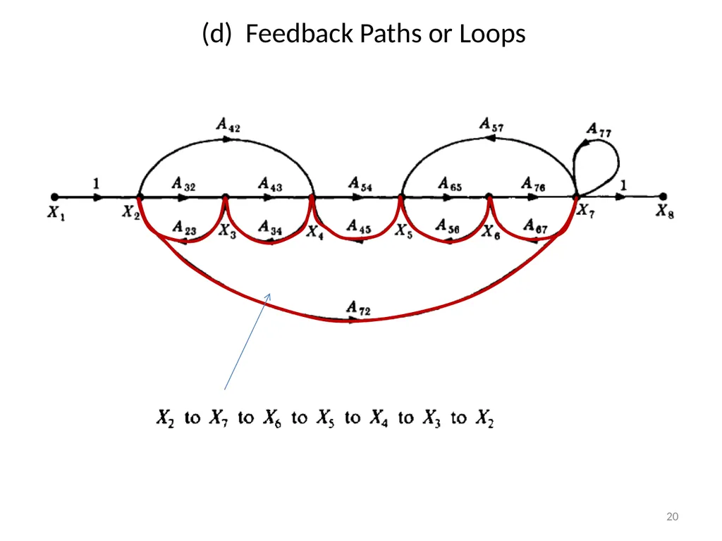
(d) Feedback Paths or Loops 20<br>
21
(e) Self Loop(s) 21<br>
22
(f) Loop Gains of the Feedback Loops 22<br>
23
(g) Path Gains of the Forward Paths 23<br>
24
Mason’s Rule (Mason, 1953) The block diagram reduction technique requires successive application of fundamental relationships in order to arrive at the system transfer function.
On the other hand, Mason’s rule for reducing a signal-flow graph to a single transfer function requires the application of one formula.
The formula was derived by S. J. Mason when he related the signal-flow graph to the simultaneous equations that can be written from the graph. 24<br>
25
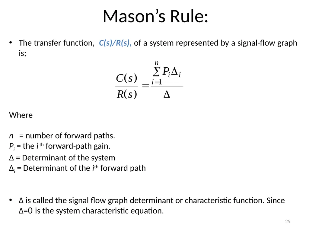
Mason’s Rule: The transfer function, C(s)/R(s), of a system represented by a signal-flow graph is;
Where
n = number of forward paths.
Pi = the i th forward-path gain.
∆ = Determinant of the system
∆i = Determinant of the ith forward path
∆ is called the signal flow graph determinant or characteristic function. Since ∆=0 is the system characteristic equation. 25<br>
26
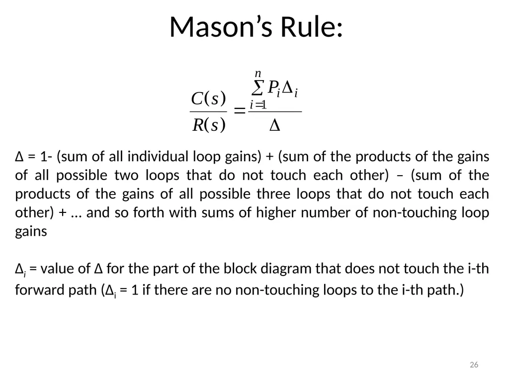
Mason’s Rule: ∆ = 1- (sum of all individual loop gains) + (sum of the products of the gains of all possible two loops that do not touch each other) – (sum of the products of the gains of all possible three loops that do not touch each other) + … and so forth with sums of higher number of non-touching loop gains
∆i = value of Δ for the part of the block diagram that does not touch the i-th forward path (Δi = 1 if there are no non-touching loops to the i-th path.) 26<br>
27
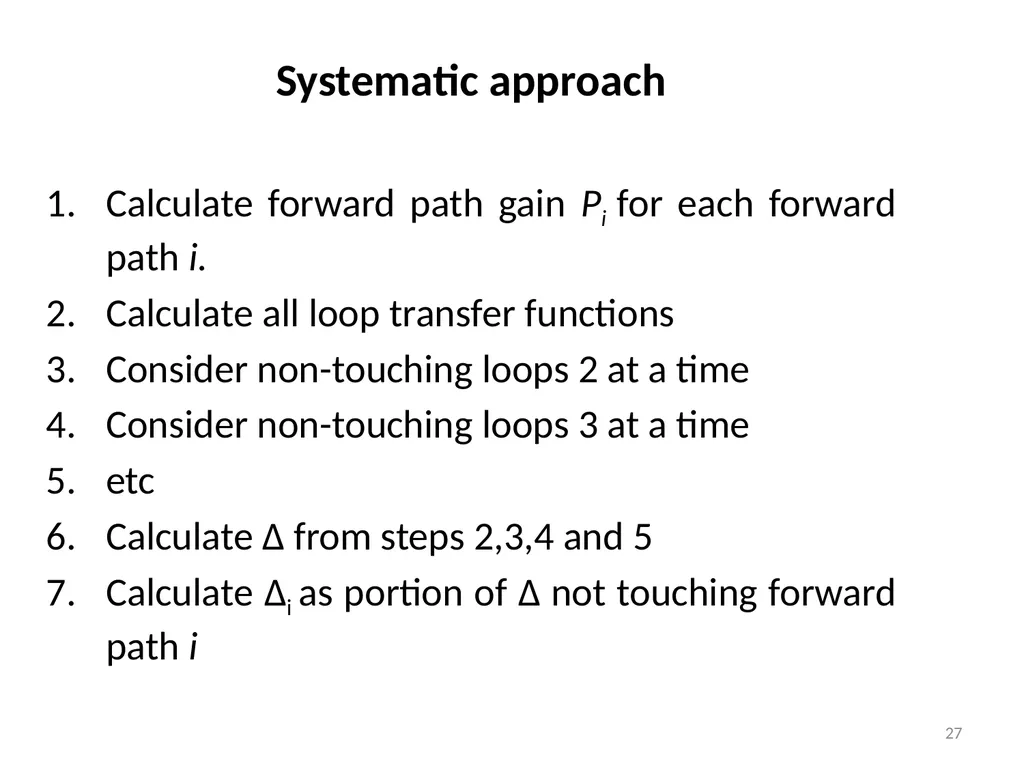
Systematic approach
Calculate forward path gain Pi for each forward path i.
Calculate all loop transfer functions
Consider non-touching loops 2 at a time
Consider non-touching loops 3 at a time
etc
Calculate Δ from steps 2,3,4 and 5
Calculate Δi as portion of Δ not touching forward path i 27<br>
28
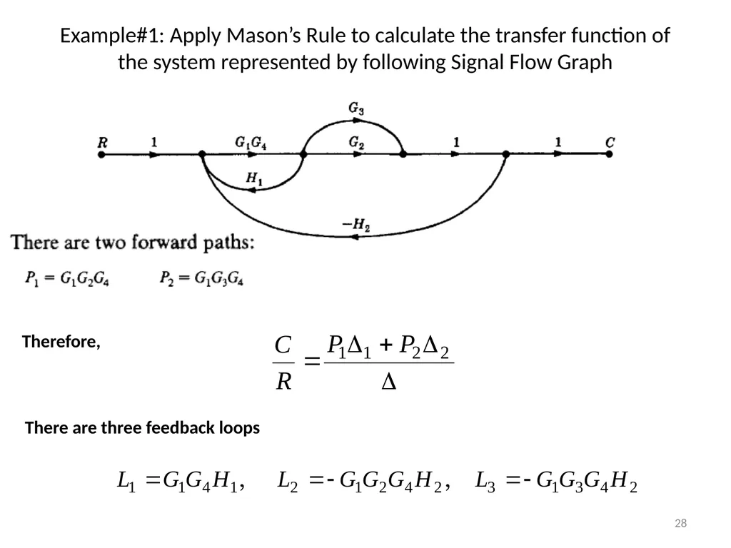
Example#1: Apply Mason’s Rule to calculate the transfer function of the system represented by following Signal Flow Graph 28<br>
29
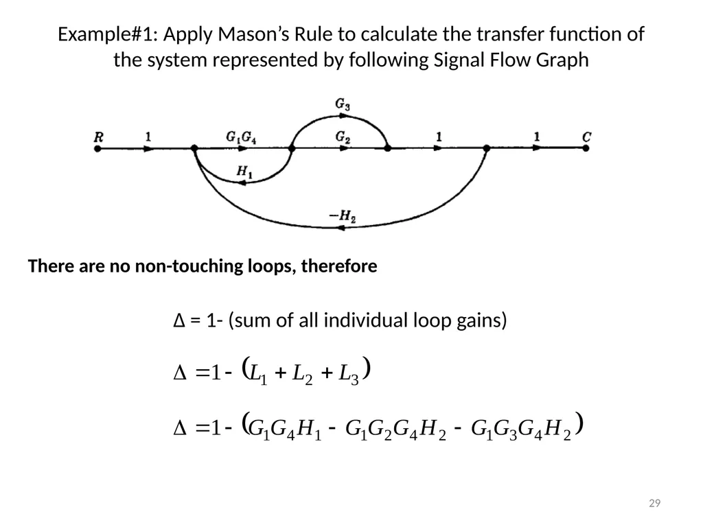
Example#1: Apply Mason’s Rule to calculate the transfer function of the system represented by following Signal Flow Graph 29<br>
30
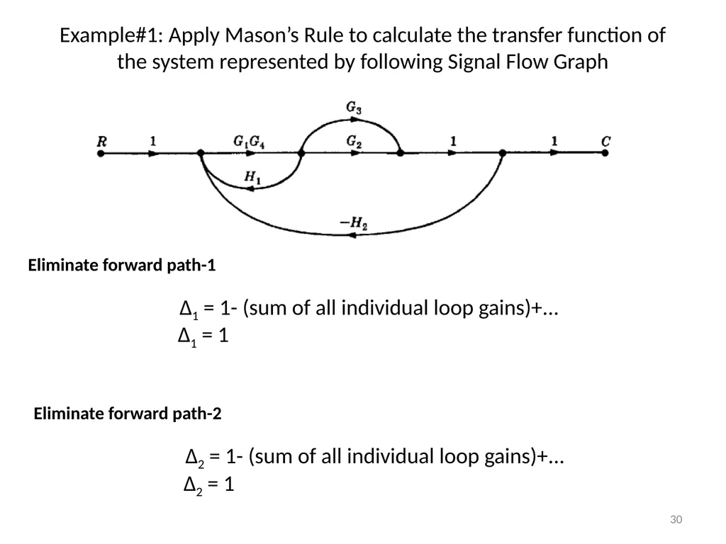
Example#1: Apply Mason’s Rule to calculate the transfer function of the system represented by following Signal Flow Graph 30<br>
31
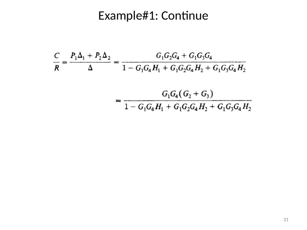
Example#1: Continue 31<br>
32
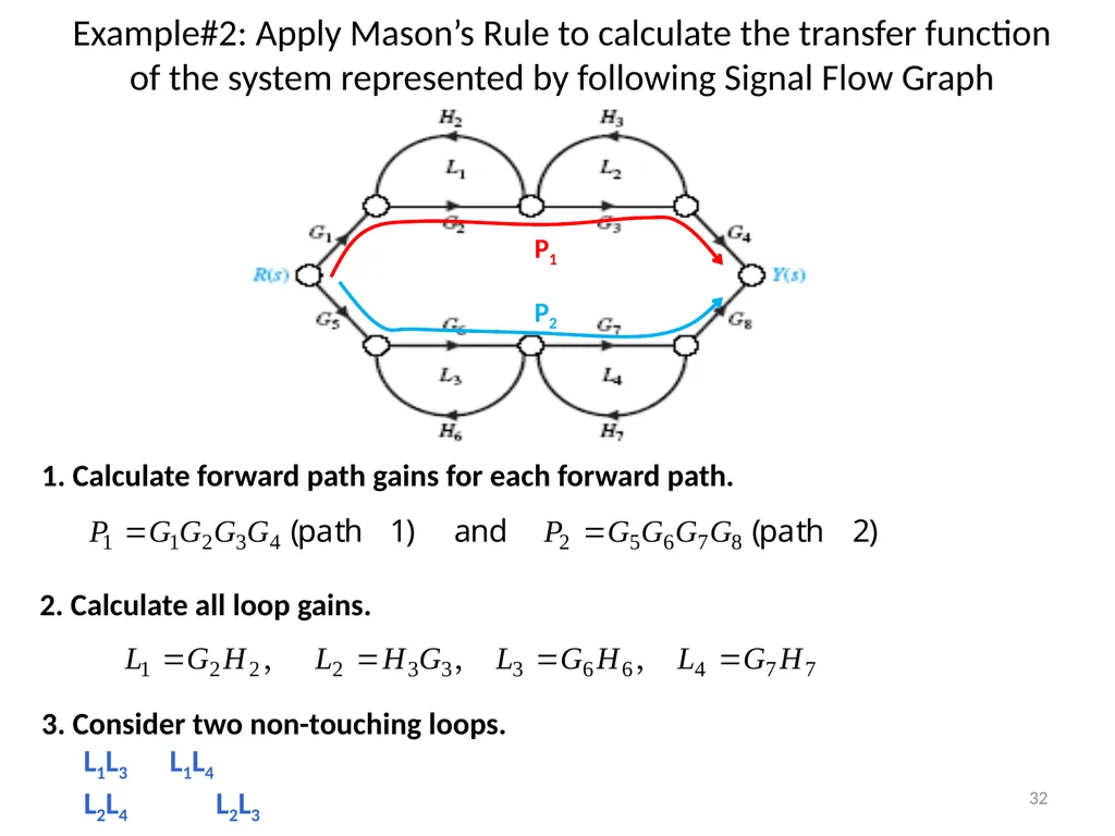
32 Example#2: Apply Mason’s Rule to calculate the transfer function of the system represented by following Signal Flow Graph 3. Consider two non-touching loops.
L1L3 L1L4
L2L4 L2L3<br>
33
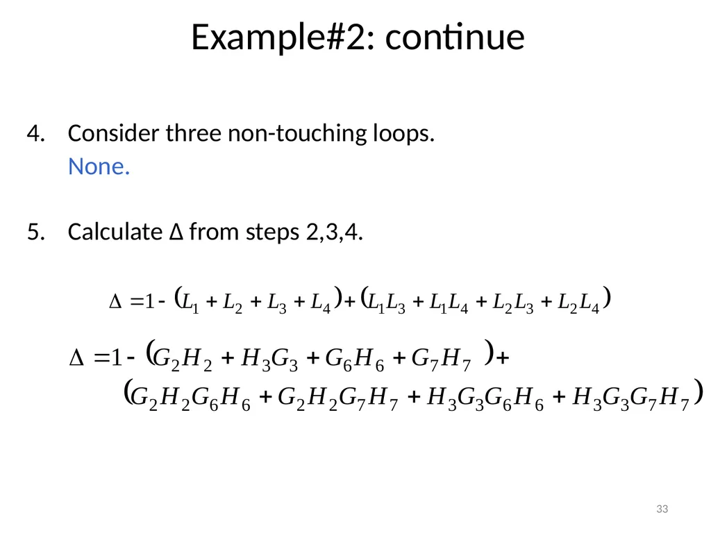
Consider three non-touching loops.
None.
Calculate Δ from steps 2,3,4. 33 Example#2: continue<br>
34
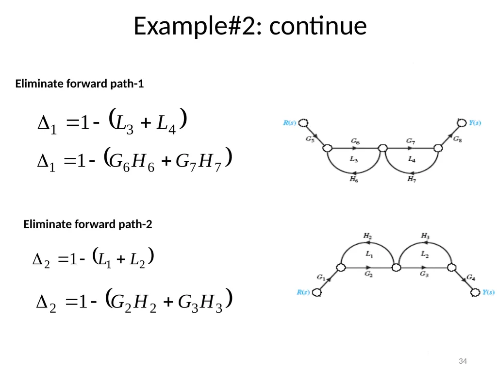
34 Example#2: continue<br>
35
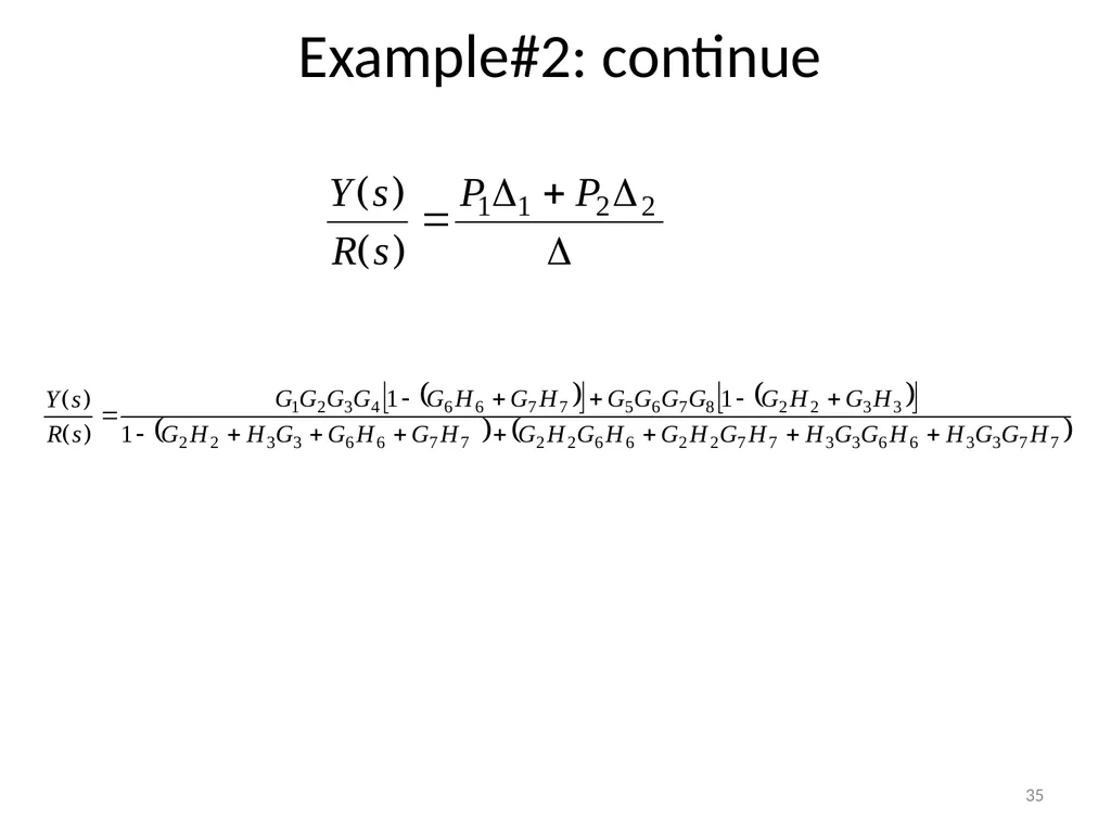
35 Example#2: continue<br>
36
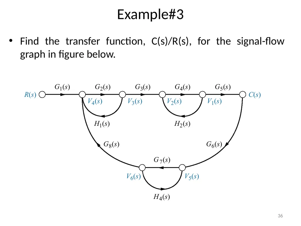
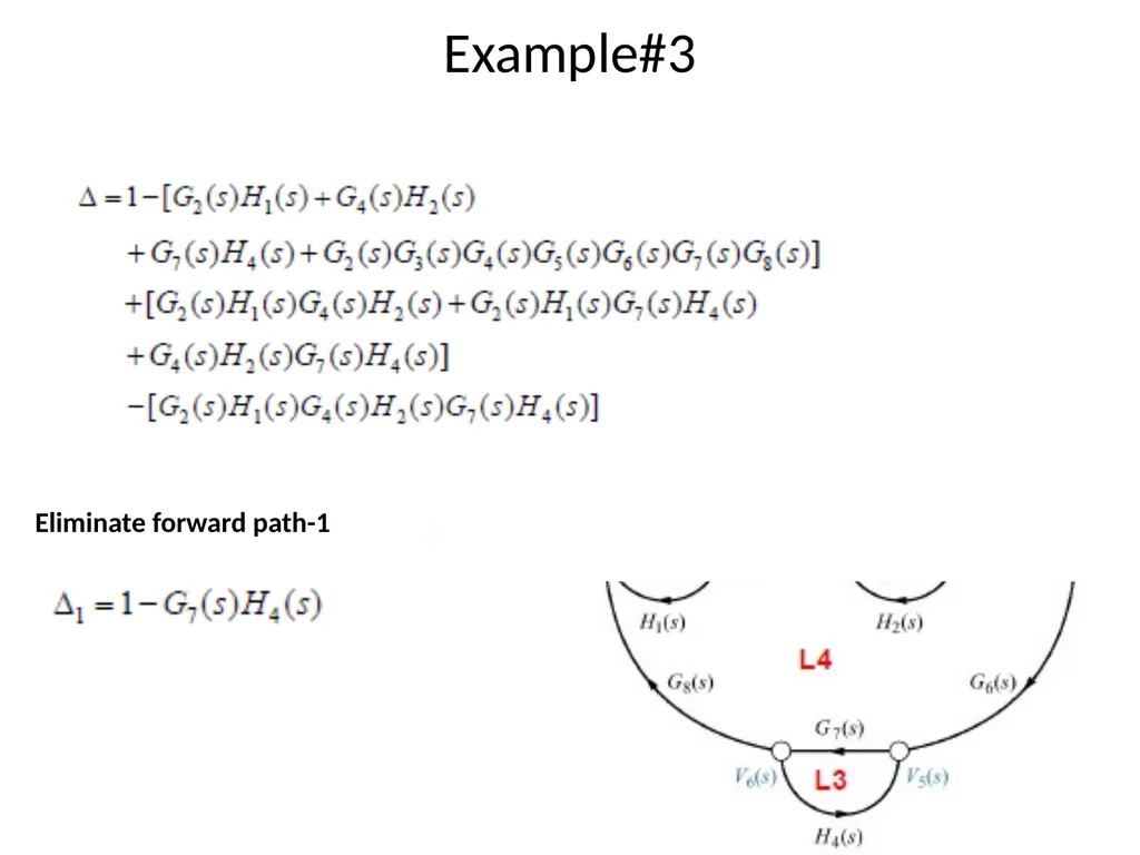
Example#3 Find the transfer function, C(s)/R(s), for the signal-flow graph in figure below. 36<br>
37
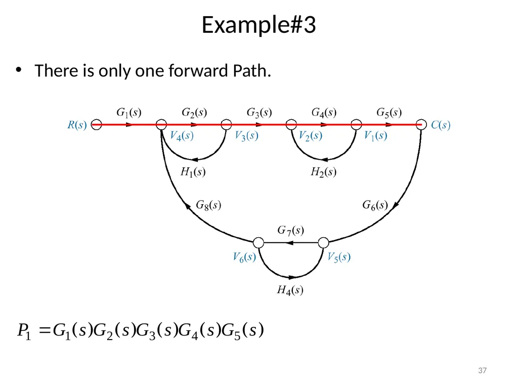
Example#3 There is only one forward Path. 37<br>
38
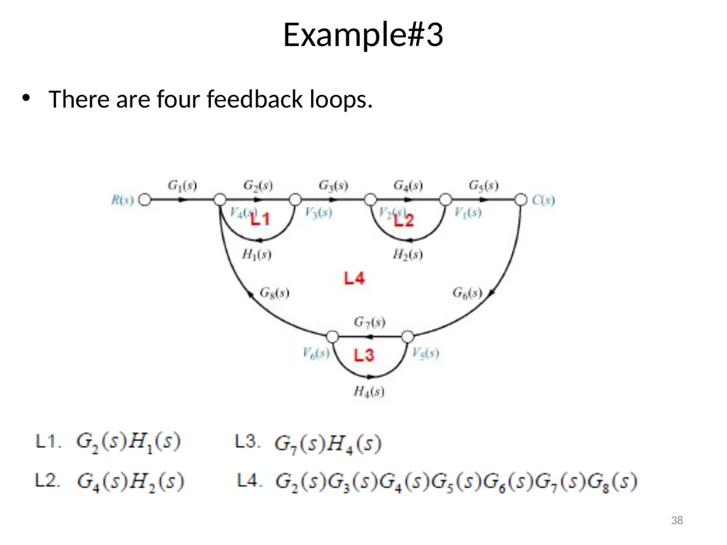
Example#3 There are four feedback loops. 38<br>
39
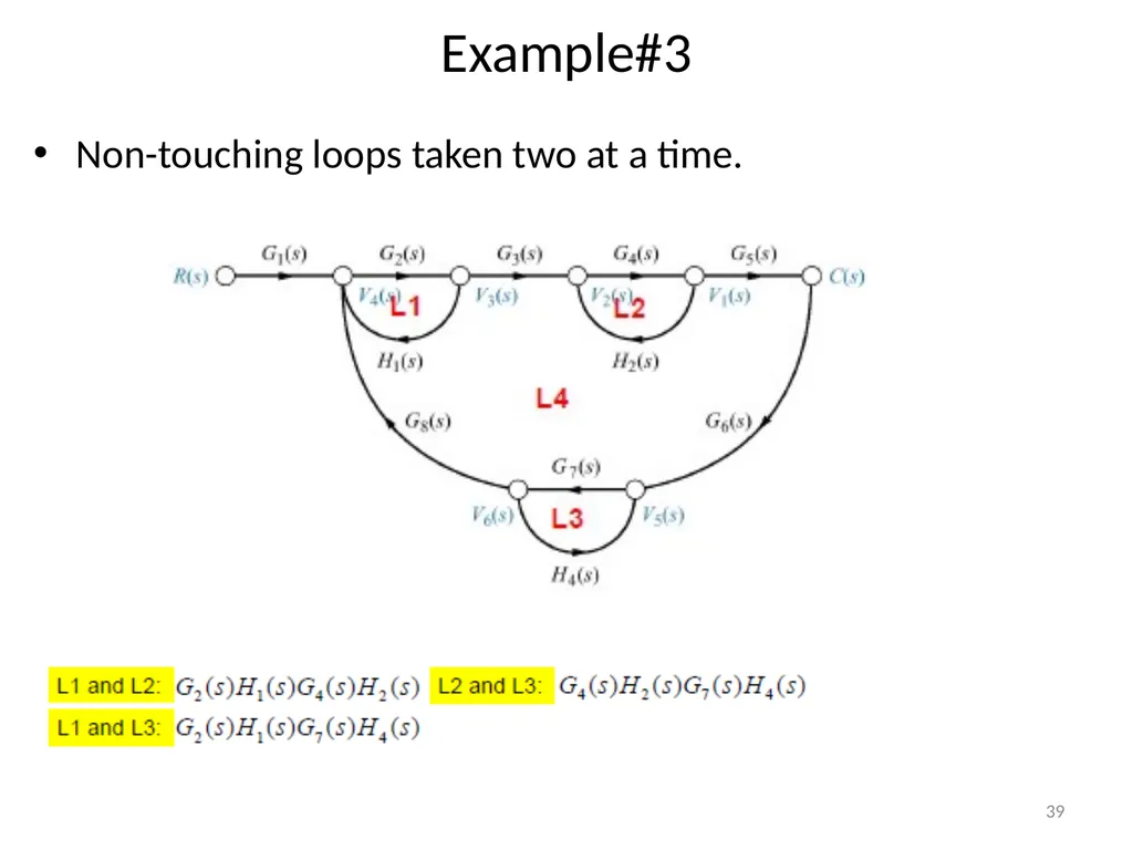
Example#3 Non-touching loops taken two at a time. 39<br>
40
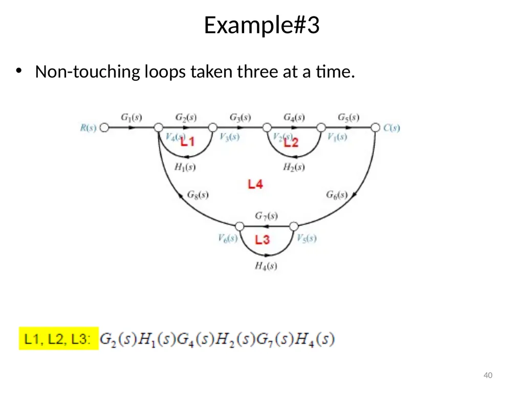
Example#3 Non-touching loops taken three at a time. 40<br>
41
Example#3 Eliminate forward path-1 41<br>
42
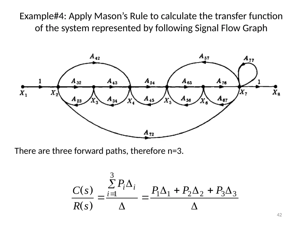
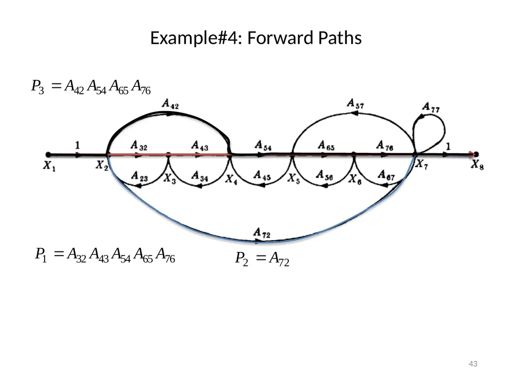
Example#4: Apply Mason’s Rule to calculate the transfer function of the system represented by following Signal Flow Graph There are three forward paths, therefore n=3. 42<br>
43
Example#4: Forward Paths 43<br>
44
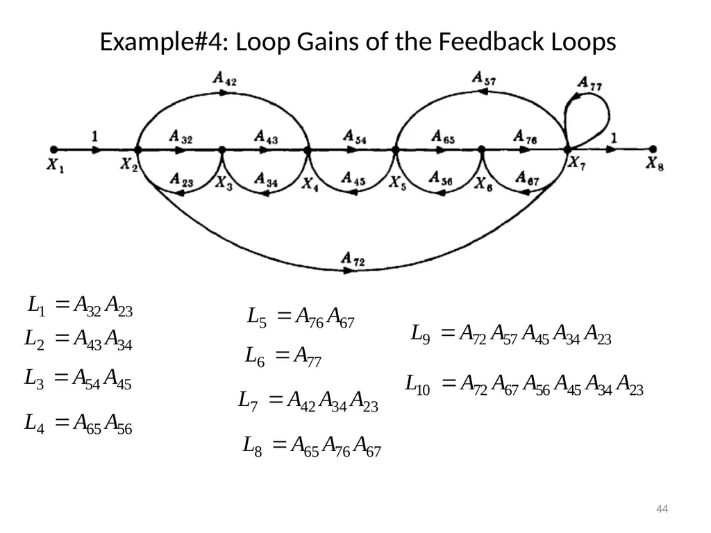
Example#4: Loop Gains of the Feedback Loops 44<br>
45
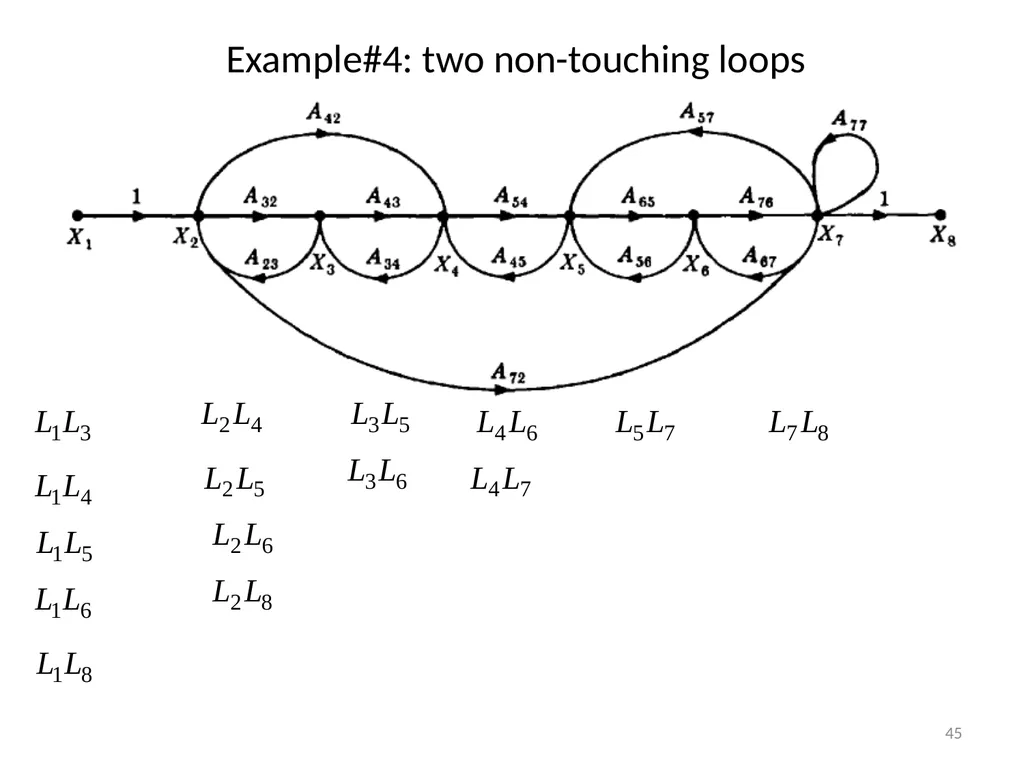
Example#4: two non-touching loops 45<br>
46
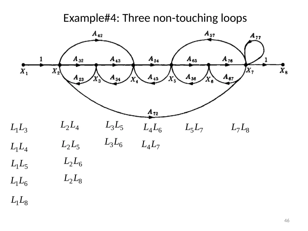
Example#4: Three non-touching loops 46<br>
47
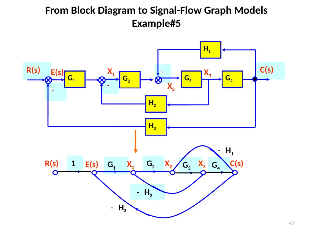
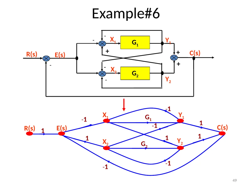
From Block Diagram to Signal-Flow Graph Models�Example#5 47<br>
48
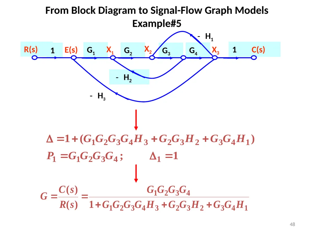
From Block Diagram to Signal-Flow Graph Models�Example#5 48<br>
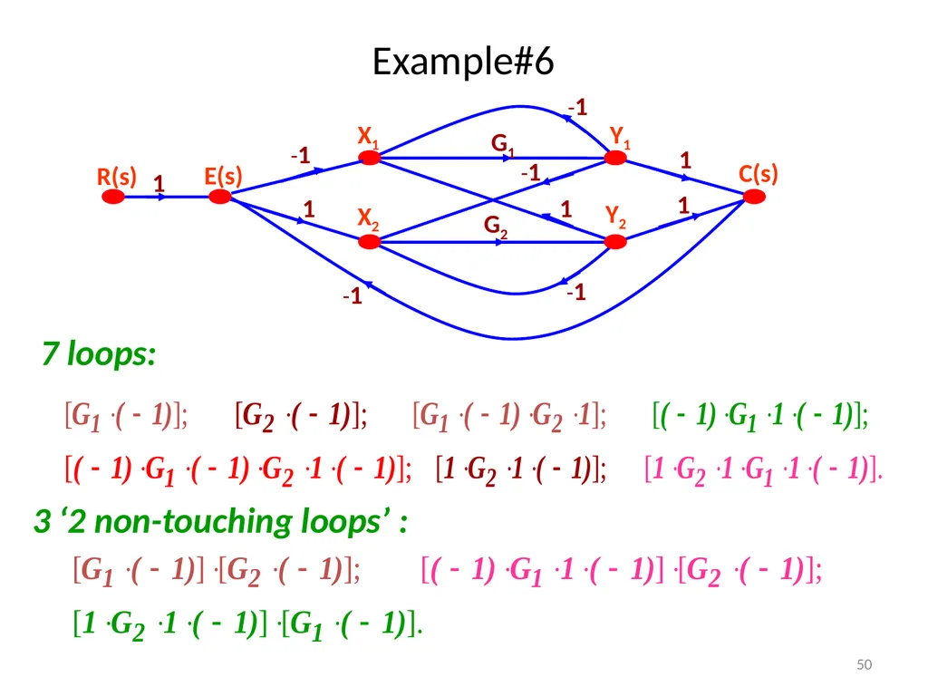
50
Example#6 7 loops: 3 ‘2 non-touching loops’ : 50<br>
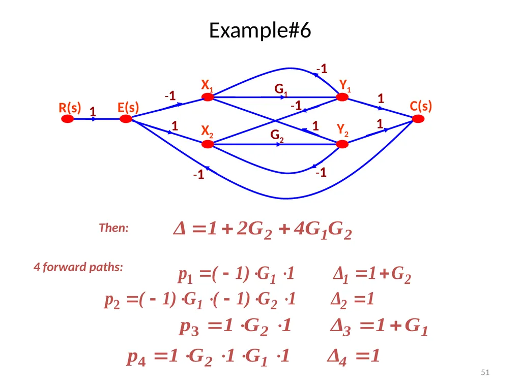
51
Example#6 Then: 4 forward paths: 51<br>
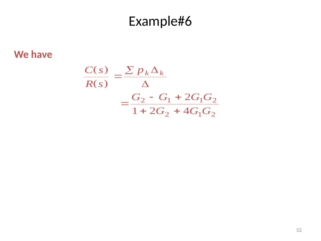
52
Example#6 We have 52<br>
53
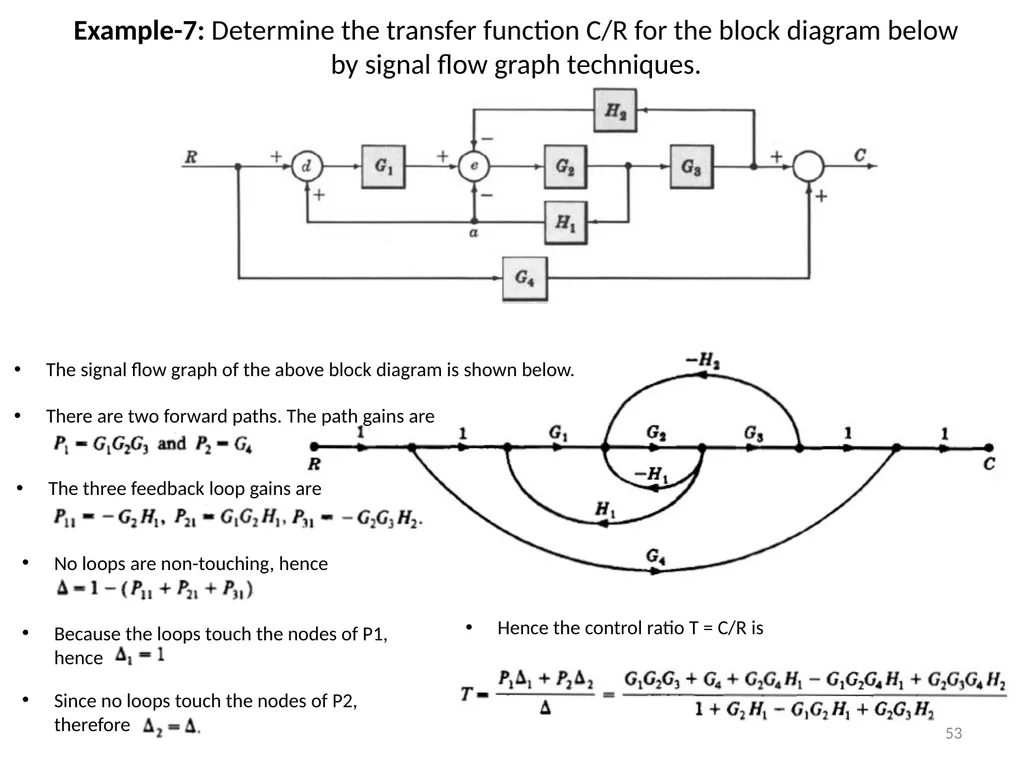
Example-7: Determine the transfer function C/R for the block diagram below by signal flow graph techniques. The signal flow graph of the above block diagram is shown below. There are two forward paths. The path gains are The three feedback loop gains are No loops are non-touching, hence Since no loops touch the nodes of P2, therefore Because the loops touch the nodes of P1, hence Hence the control ratio T = C/R is 53<br>
54
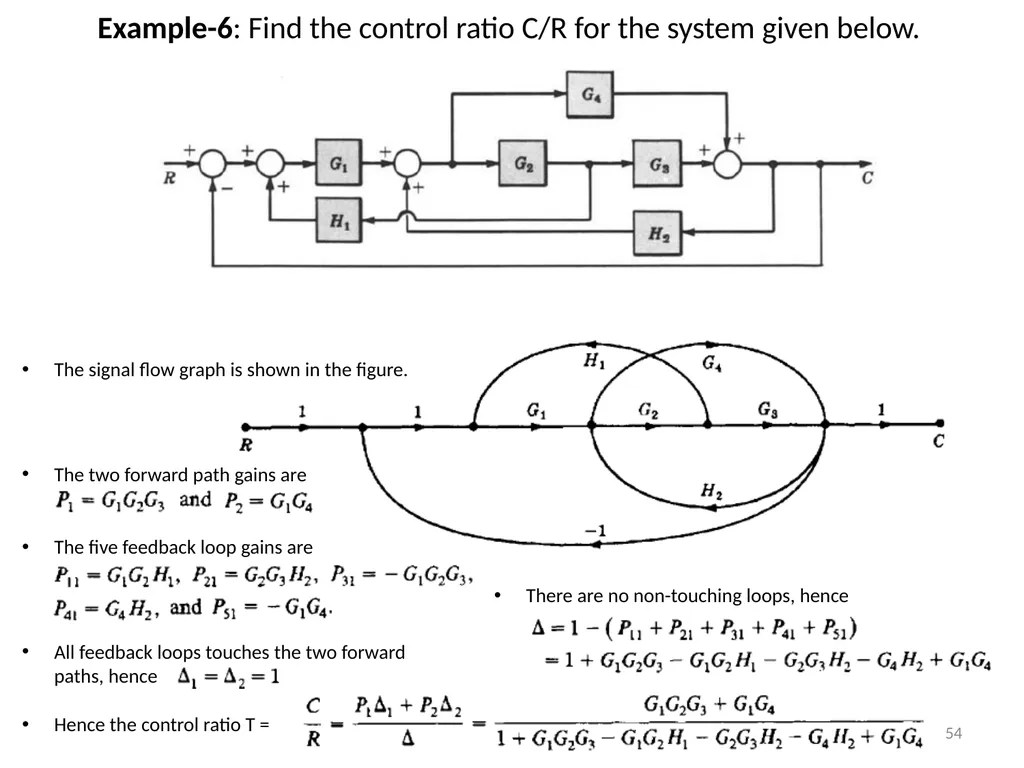
Example-6: Find the control ratio C/R for the system given below. The two forward path gains are The signal flow graph is shown in the figure. The five feedback loop gains are Hence the control ratio T = There are no non-touching loops, hence All feedback loops touches the two forward paths, hence 54<br>
55
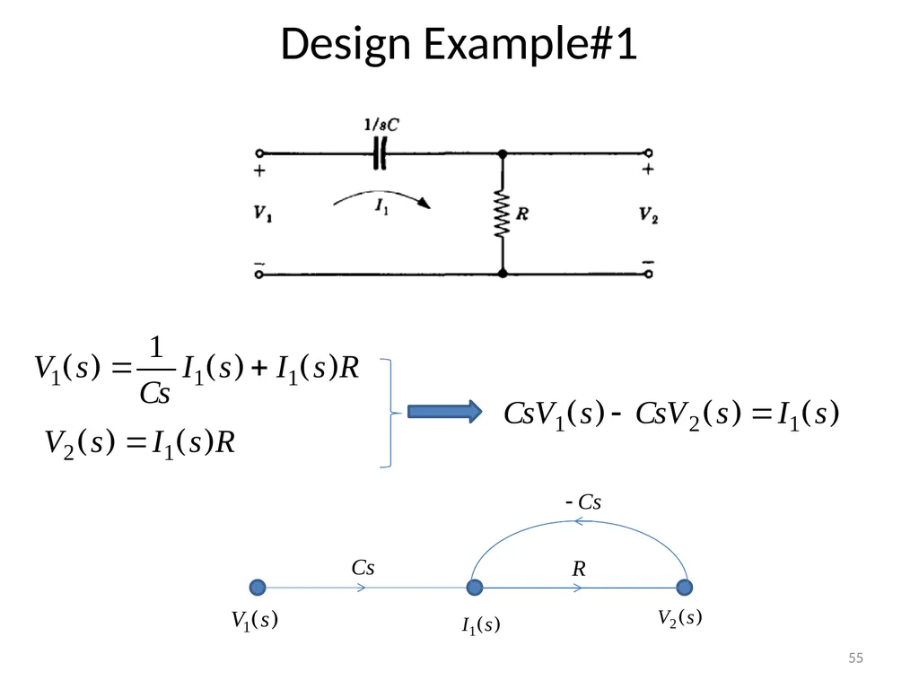
Design Example#1 55<br>
56
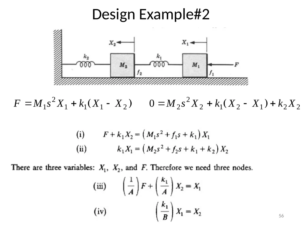
Design Example#2 56<br>
57
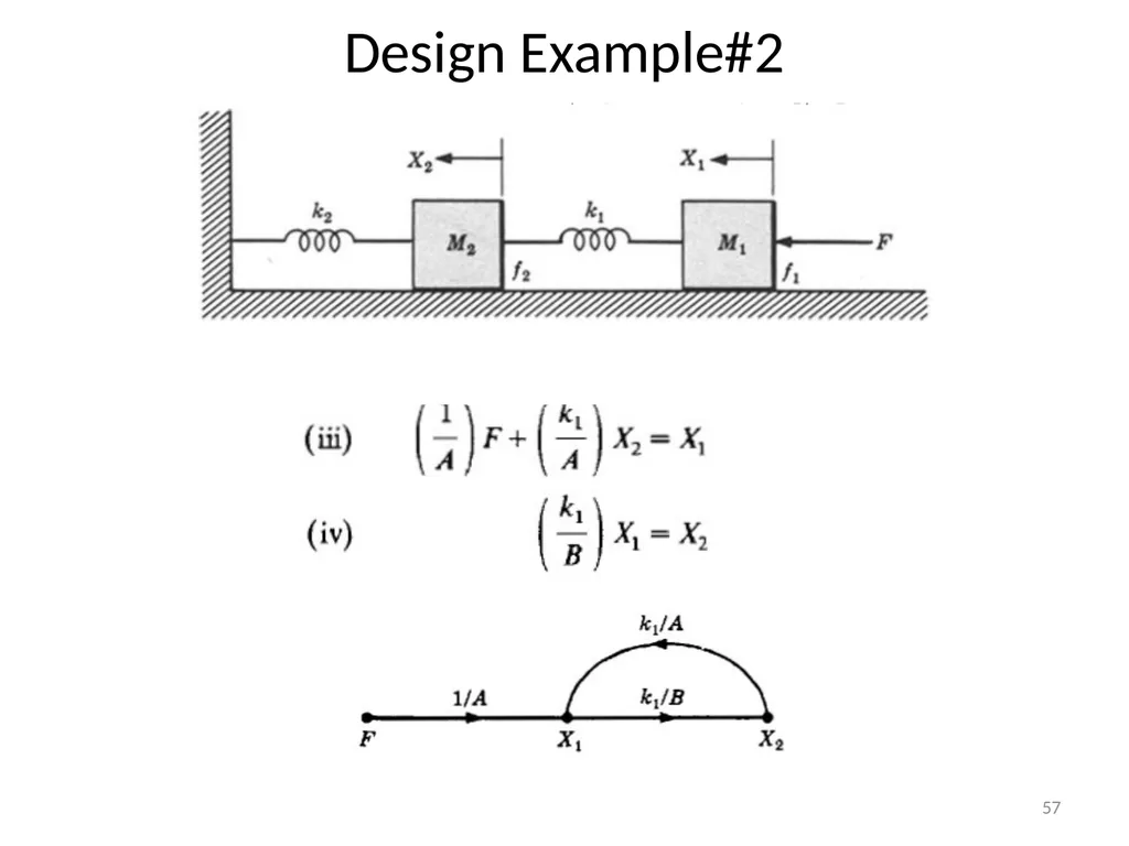
Design Example#2 57<br>
58
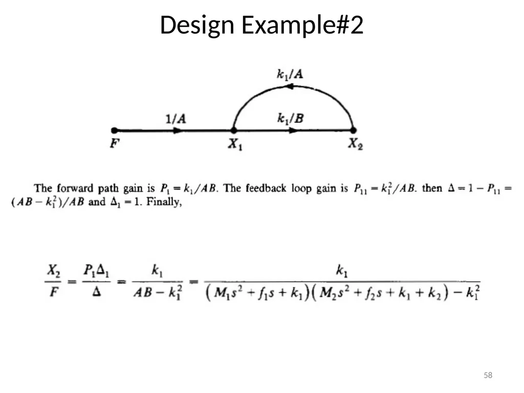
Design Example#2 58<br>
59
End of Lecture-4 To download this lecture visit
http://imtiazhussainkalwar.weebly.com/ 59<br>