
Econometrics I Professor William Greene Stern
GB
Published · 51 slides · 0 views

1 / 1




Description
Econometrics I Professor William Greene Stern School of Business Department of Economics Econometrics I Part 13 Endogeneity: Applications Measurement Error y x all of the usual assumptions x x u the true x is not observed
Related Topics
Share
Embed code
Download this presentation From Below
"Econometrics I Professor William Greene Stern" is the property of its rightful owner. Permission is granted to download and print the materials on this website for personal, non-commercial use only, and to display it on your personal computer provided you do not modify the materials and that you retain all copyright notices contained in the materials. By downloading content from our website, you accept the terms of this agreement.
Presentation Transcript
01
Econometrics I Professor William Greene
Stern School of Business
Department of Economics<br>
Stern School of Business
Department of Economics<br>
02
Econometrics I Part 13 – Endogeneity:
Applications<br>
03
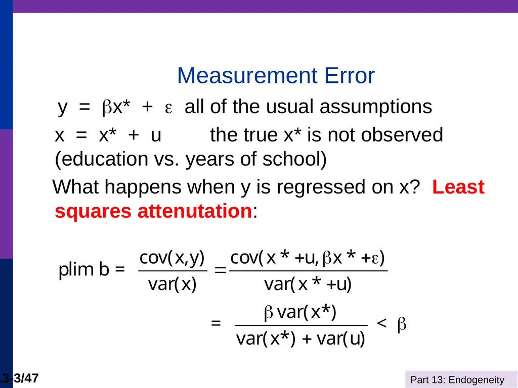
Measurement Error y = x* + all of the usual assumptions
x = x* + u the true x* is not observed (education vs. years of school)
What happens when y is regressed on x? Least squares attenutation:<br>
x = x* + u the true x* is not observed (education vs. years of school)
What happens when y is regressed on x? Least squares attenutation:<br>
04
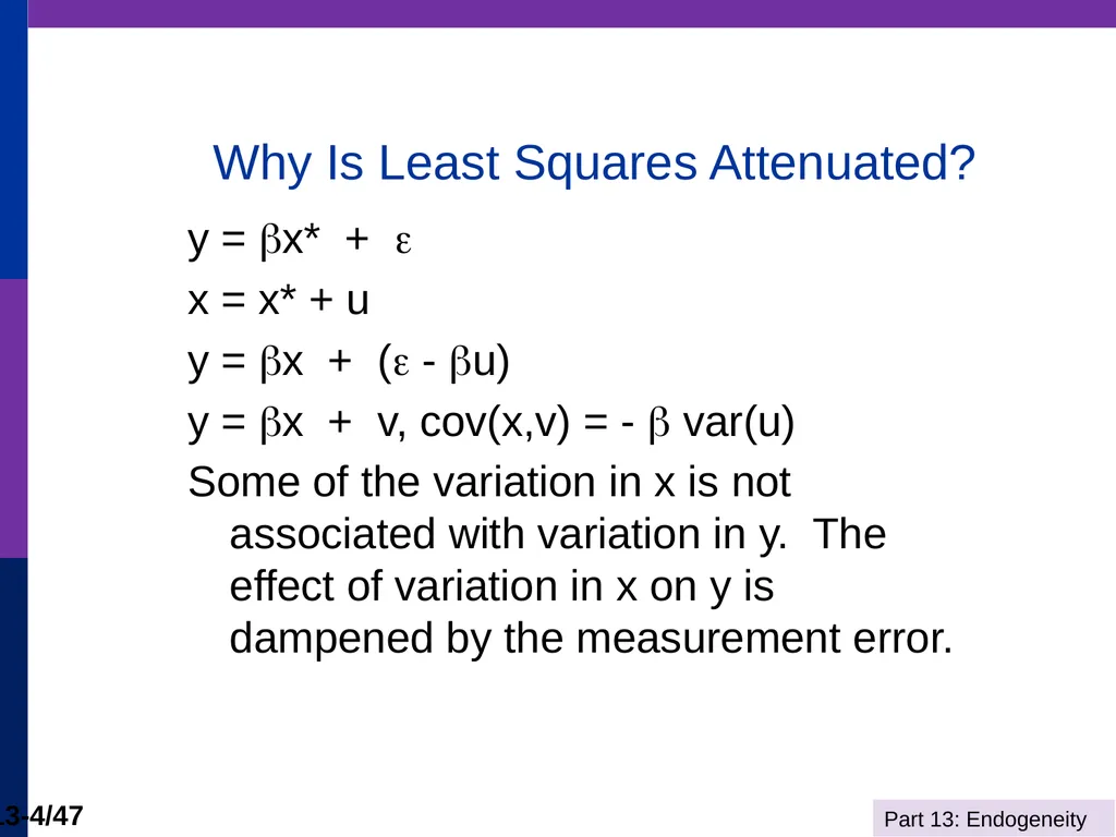
Why Is Least Squares Attenuated? y = x* +
x = x* + u
y = x + ( - u)
y = x + v, cov(x,v) = - var(u)
Some of the variation in x is not associated with variation in y. The effect of variation in x on y is dampened by the measurement error.<br>
x = x* + u
y = x + ( - u)
y = x + v, cov(x,v) = - var(u)
Some of the variation in x is not associated with variation in y. The effect of variation in x on y is dampened by the measurement error.<br>
05
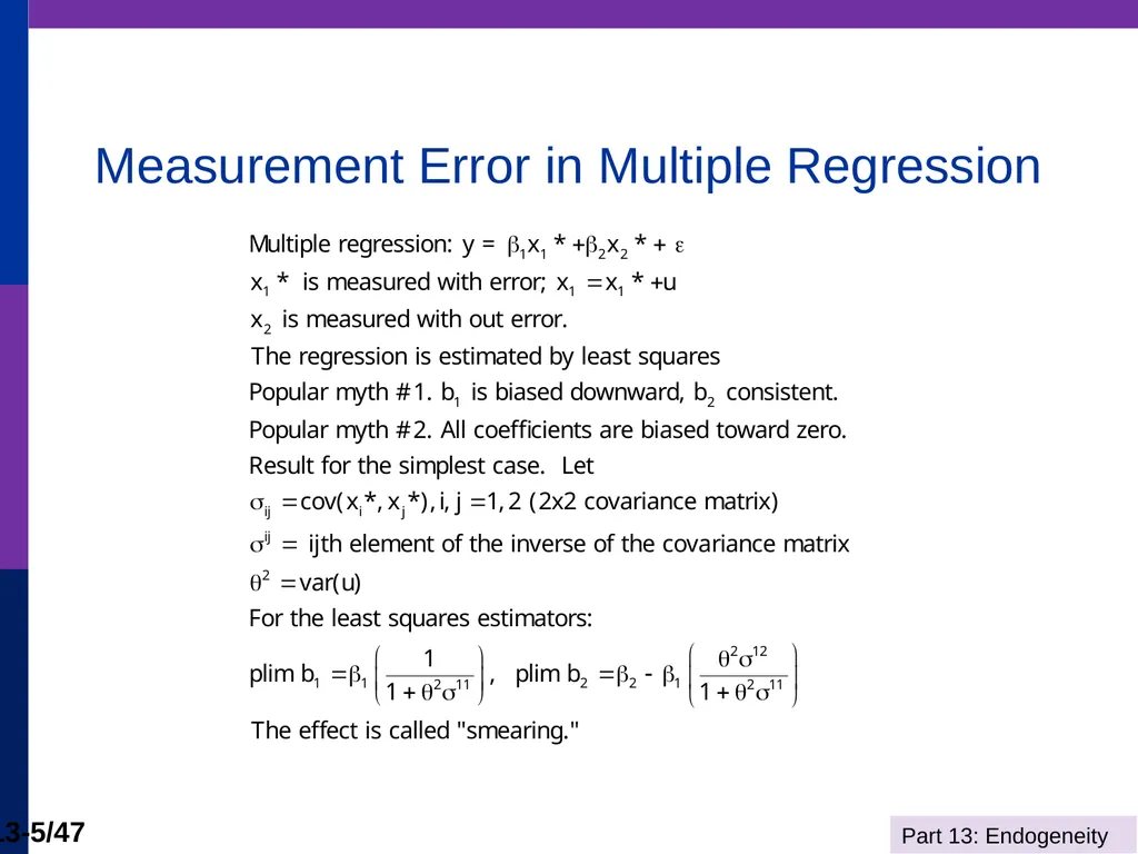
Measurement Error in Multiple Regression<br>
06
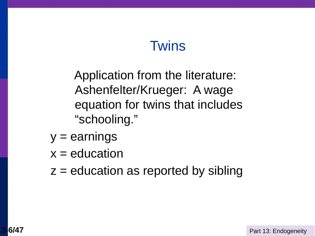
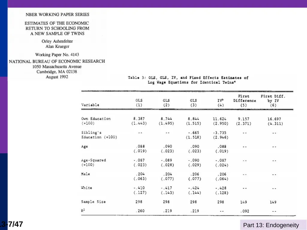
Twins Application from the literature: Ashenfelter/Krueger: A wage equation for twins that includes “schooling.”
y = earnings
x = education
z = education as reported by sibling<br>
y = earnings
x = education
z = education as reported by sibling<br>
07
Orthodoxy A proxy is not an instrumental variable
Instrument is a noun, not a verb
Are you sure that the instrument is really exogenous? The “natural experiment.”<br>
Instrument is a noun, not a verb
Are you sure that the instrument is really exogenous? The “natural experiment.”<br>
08
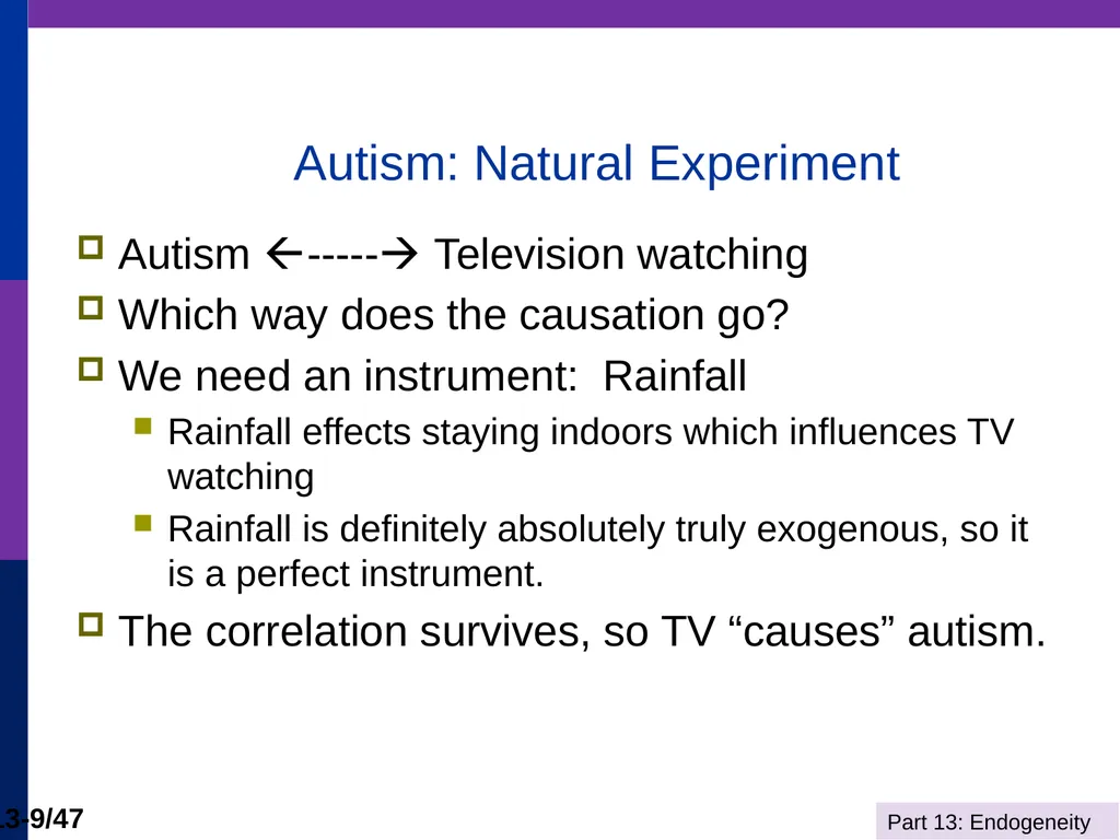
Autism: Natural Experiment Autism ----- Television watching
Which way does the causation go?
We need an instrument: Rainfall
Rainfall effects staying indoors which influences TV watching
Rainfall is definitely absolutely truly exogenous, so it is a perfect instrument.
The correlation survives, so TV “causes” autism.<br>
Which way does the causation go?
We need an instrument: Rainfall
Rainfall effects staying indoors which influences TV watching
Rainfall is definitely absolutely truly exogenous, so it is a perfect instrument.
The correlation survives, so TV “causes” autism.<br>
09
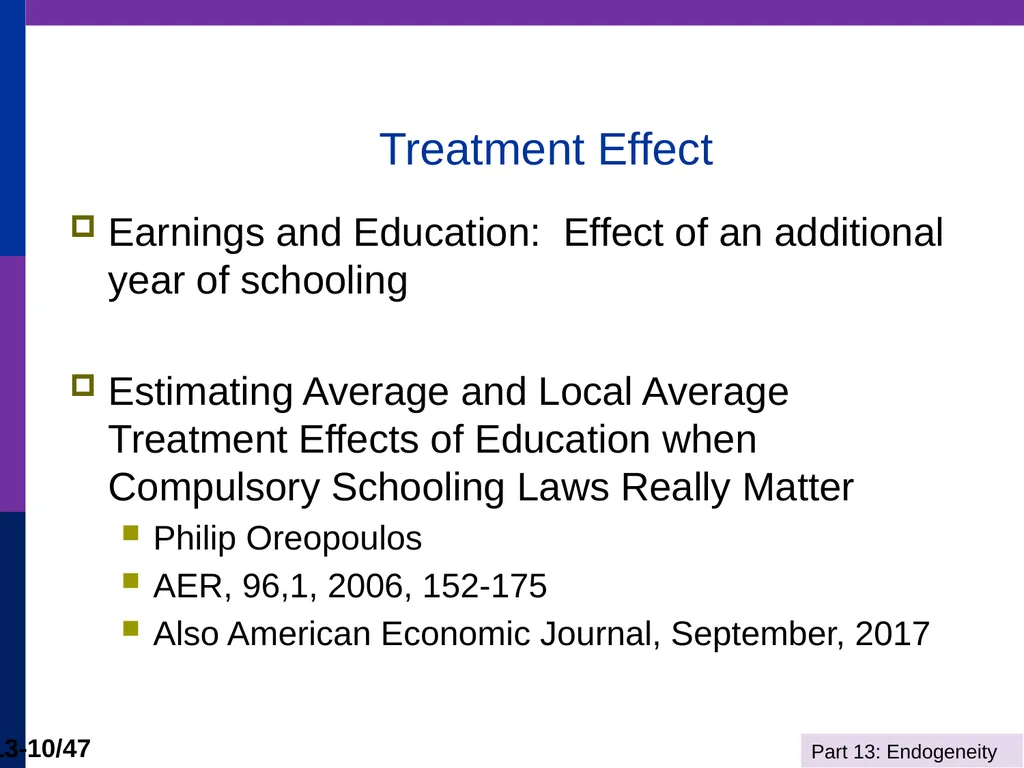
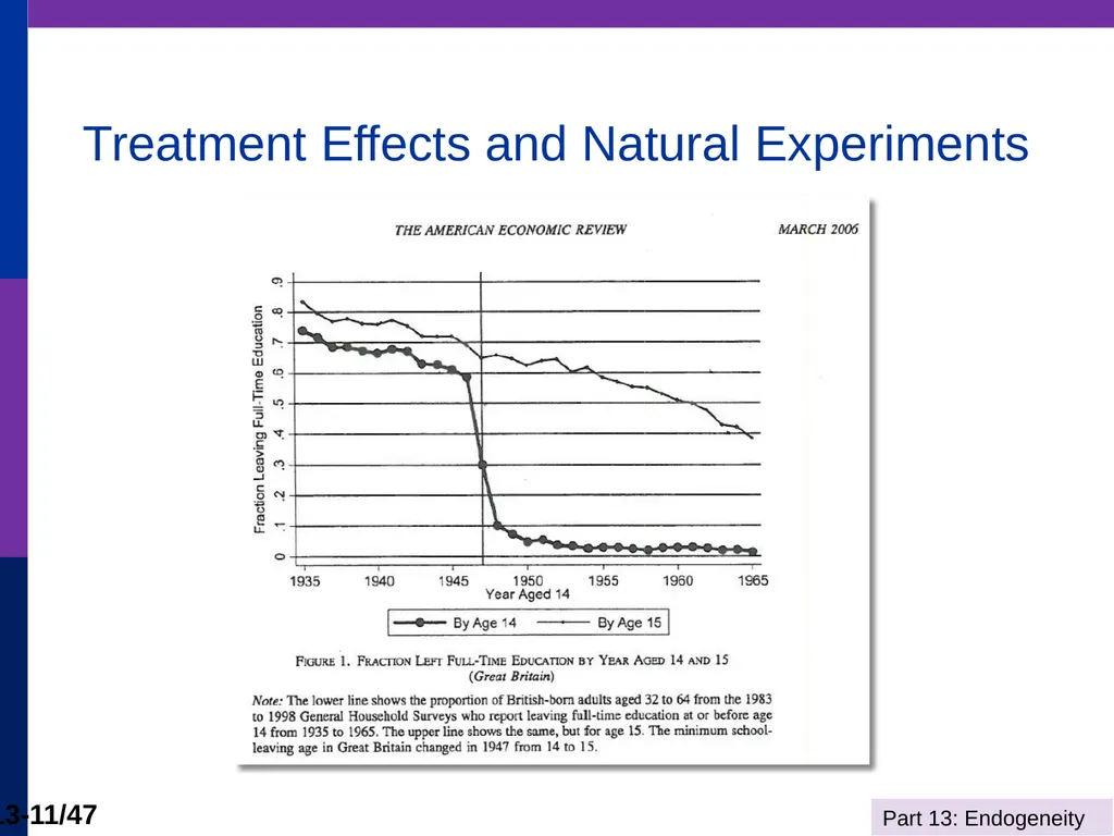
Treatment Effect Earnings and Education: Effect of an additional year of schooling
Estimating Average and Local Average Treatment Effects of Education when Compulsory Schooling Laws Really Matter
Philip Oreopoulos
AER, 96,1, 2006, 152-175
Also American Economic Journal, September, 2017<br>
Estimating Average and Local Average Treatment Effects of Education when Compulsory Schooling Laws Really Matter
Philip Oreopoulos
AER, 96,1, 2006, 152-175
Also American Economic Journal, September, 2017<br>
10
Treatment Effects and Natural Experiments<br>
11
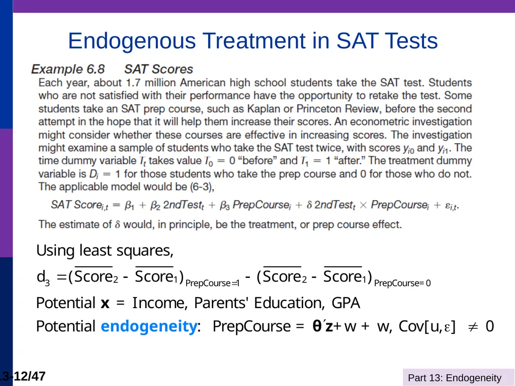
Endogenous Treatment in SAT Tests<br>
12
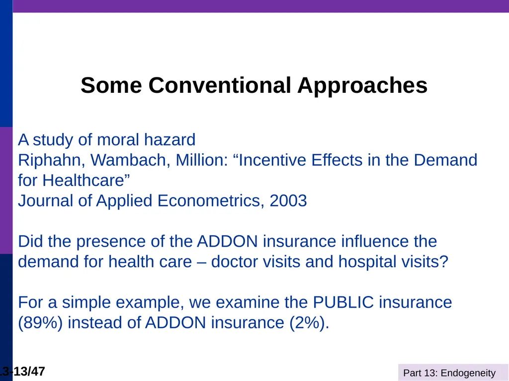
A study of moral hazard
Riphahn, Wambach, Million: “Incentive Effects in the Demand for Healthcare”
Journal of Applied Econometrics, 2003
Did the presence of the ADDON insurance influence the demand for health care – doctor visits and hospital visits?
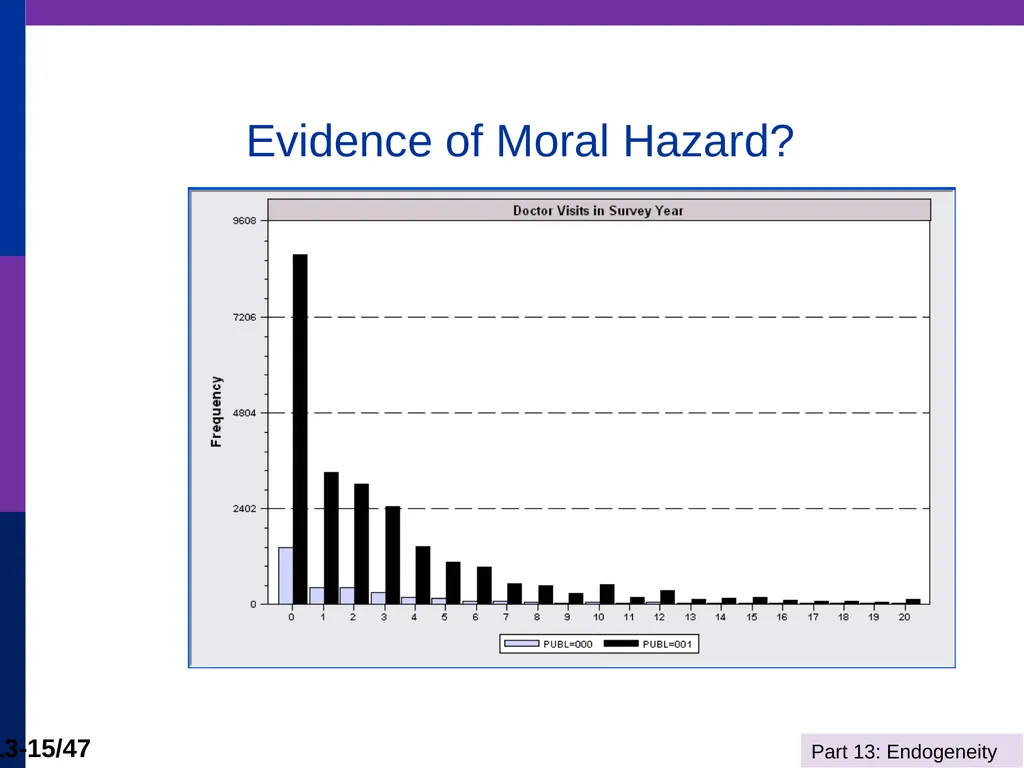
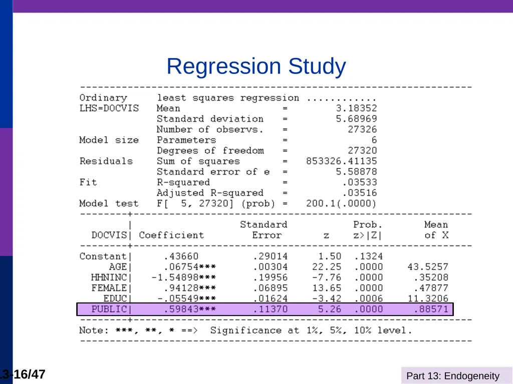
For a simple example, we examine the PUBLIC insurance (89%) instead of ADDON insurance (2%). Some Conventional Approaches<br>
13
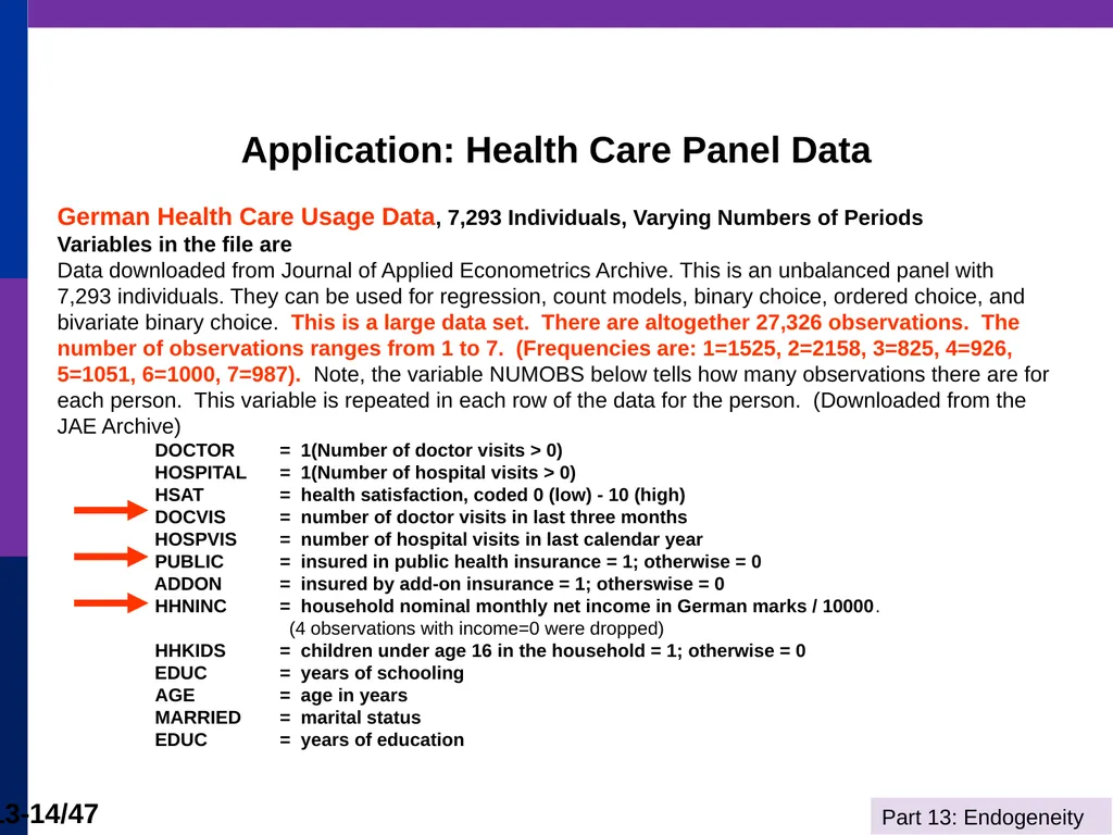
Application: Health Care Panel Data German Health Care Usage Data, 7,293 Individuals, Varying Numbers of Periods
Variables in the file are
Data downloaded from Journal of Applied Econometrics Archive. This is an unbalanced panel with 7,293 individuals. They can be used for regression, count models, binary choice, ordered choice, and bivariate binary choice. This is a large data set. There are altogether 27,326 observations. The number of observations ranges from 1 to 7. (Frequencies are: 1=1525, 2=2158, 3=825, 4=926, 5=1051, 6=1000, 7=987). Note, the variable NUMOBS below tells how many observations there are for each person. This variable is repeated in each row of the data for the person. (Downloaded from the JAE Archive)
DOCTOR = 1(Number of doctor visits > 0) HOSPITAL = 1(Number of hospital visits > 0)
HSAT = health satisfaction, coded 0 (low) - 10 (high)
DOCVIS = number of doctor visits in last three months HOSPVIS = number of hospital visits in last calendar year PUBLIC = insured in public health insurance = 1; otherwise = 0 ADDON = insured by add-on insurance = 1; otherswise = 0
HHNINC = household nominal monthly net income in German marks / 10000.
(4 observations with income=0 were dropped) HHKIDS = children under age 16 in the household = 1; otherwise = 0 EDUC = years of schooling
AGE = age in years
MARRIED = marital status
EDUC = years of education<br>
DOCTOR = 1(Number of doctor visits > 0) HOSPITAL = 1(Number of hospital visits > 0)
HSAT = health satisfaction, coded 0 (low) - 10 (high)
DOCVIS = number of doctor visits in last three months HOSPVIS = number of hospital visits in last calendar year PUBLIC = insured in public health insurance = 1; otherwise = 0 ADDON = insured by add-on insurance = 1; otherswise = 0
HHNINC = household nominal monthly net income in German marks / 10000.
(4 observations with income=0 were dropped) HHKIDS = children under age 16 in the household = 1; otherwise = 0 EDUC = years of schooling
AGE = age in years
MARRIED = marital status
EDUC = years of education<br>
14
Evidence of Moral Hazard?<br>
15
Regression Study<br>
16
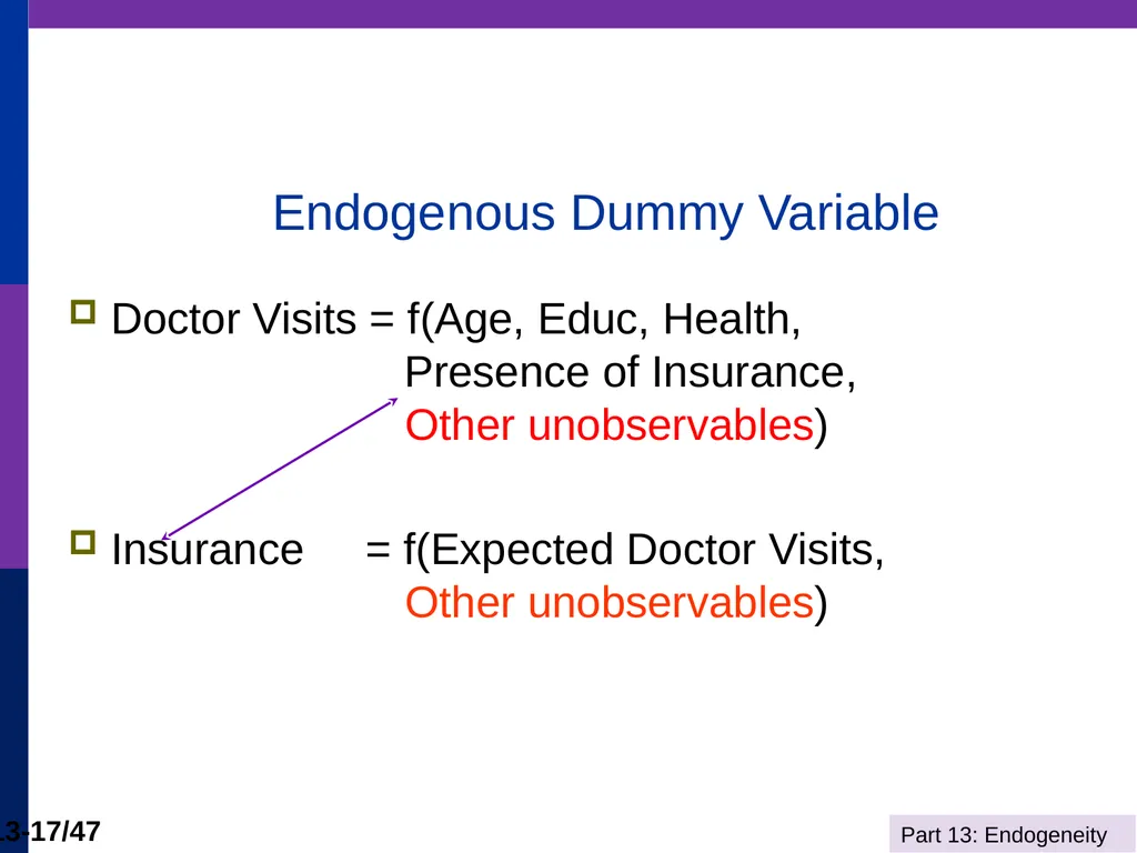
Endogenous Dummy Variable Doctor Visits = f(Age, Educ, Health,
Presence of Insurance,
Other unobservables)
Insurance = f(Expected Doctor Visits, Other unobservables)<br>
Insurance = f(Expected Doctor Visits, Other unobservables)<br>
17
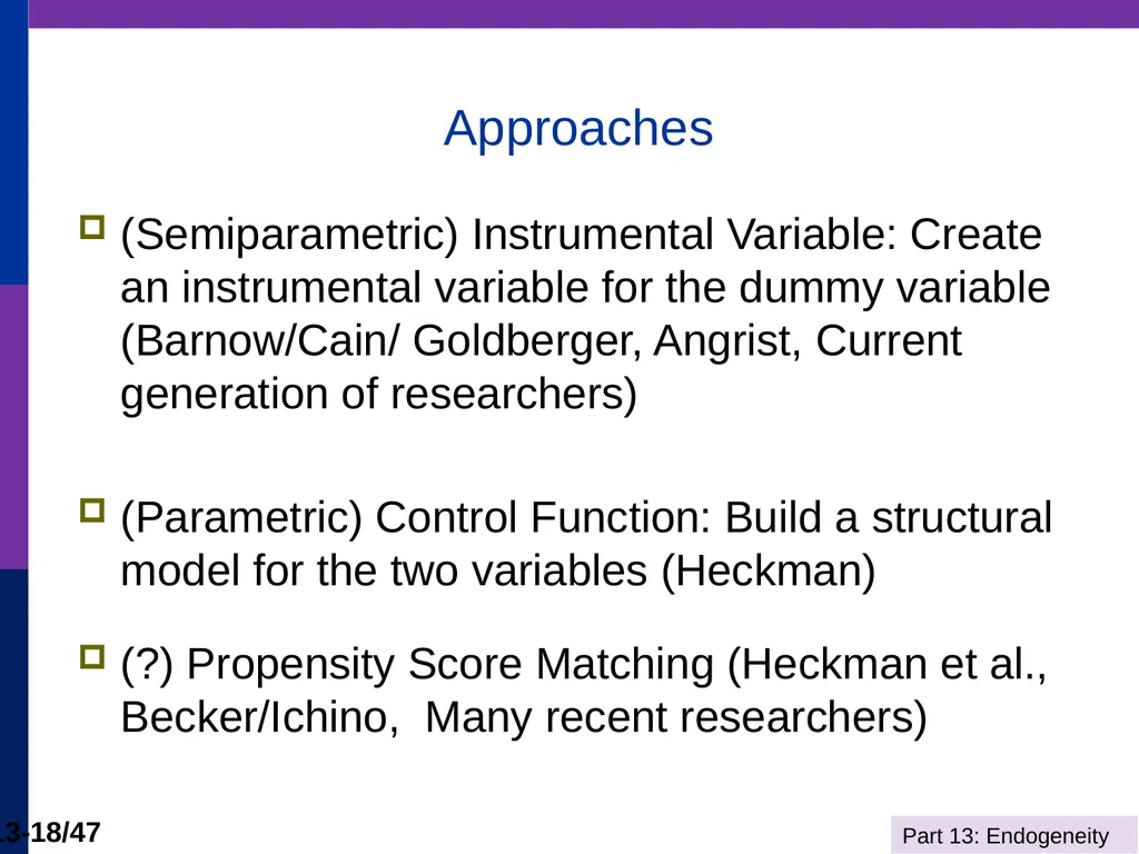
Approaches (Semiparametric) Instrumental Variable: Create an instrumental variable for the dummy variable (Barnow/Cain/ Goldberger, Angrist, Current generation of researchers)
(Parametric) Control Function: Build a structural model for the two variables (Heckman)
(?) Propensity Score Matching (Heckman et al., Becker/Ichino, Many recent researchers)<br>
(Parametric) Control Function: Build a structural model for the two variables (Heckman)
(?) Propensity Score Matching (Heckman et al., Becker/Ichino, Many recent researchers)<br>
18
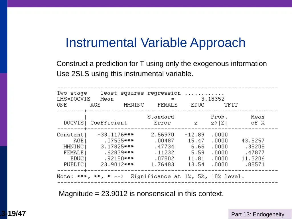
Instrumental Variable Approach Construct a prediction for T using only the exogenous information
Use 2SLS using this instrumental variable. Magnitude = 23.9012 is nonsensical in this context.<br>
Use 2SLS using this instrumental variable. Magnitude = 23.9012 is nonsensical in this context.<br>
19
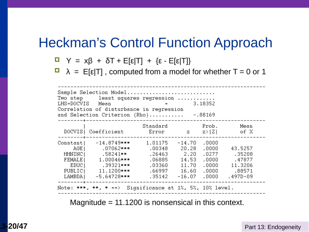
Heckman’s Control Function Approach Y = xβ + δT + E[ε|T] + {ε - E[ε|T]}
λ = E[ε|T] , computed from a model for whether T = 0 or 1 Magnitude = 11.1200 is nonsensical in this context.<br>
λ = E[ε|T] , computed from a model for whether T = 0 or 1 Magnitude = 11.1200 is nonsensical in this context.<br>
20
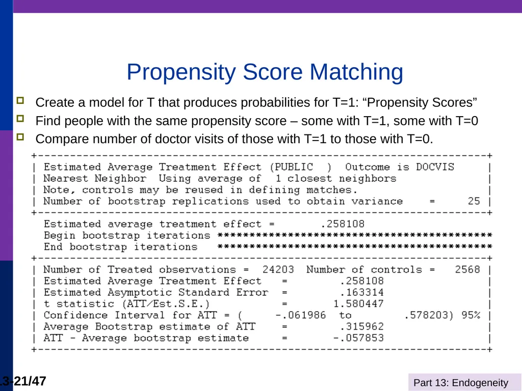
Propensity Score Matching Create a model for T that produces probabilities for T=1: “Propensity Scores”
Find people with the same propensity score – some with T=1, some with T=0
Compare number of doctor visits of those with T=1 to those with T=0.<br>
Find people with the same propensity score – some with T=1, some with T=0
Compare number of doctor visits of those with T=1 to those with T=0.<br>
21
Application of a Two Period Model “Hemoglobin and Quality of Life in Cancer Patients with Anemia,”
Finkelstein (MIT), Berndt (MIT), Greene (NYU), Cremieux (Univ. of Quebec)
1998
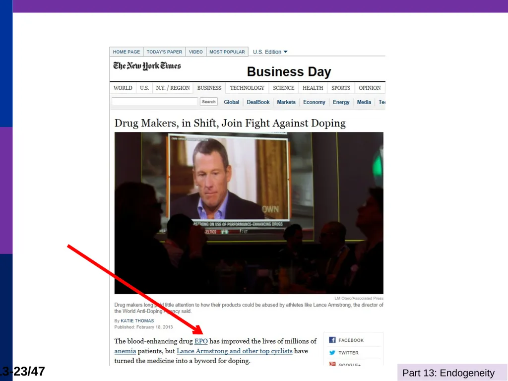
With Ortho Biotech – seeking to change labeling of already approved drug ‘erythropoetin.’ r-HuEPO<br>
Finkelstein (MIT), Berndt (MIT), Greene (NYU), Cremieux (Univ. of Quebec)
1998
With Ortho Biotech – seeking to change labeling of already approved drug ‘erythropoetin.’ r-HuEPO<br>
22
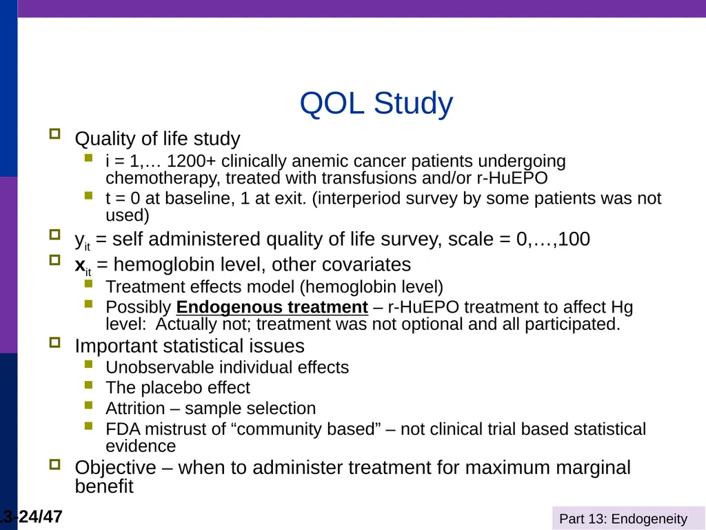
QOL Study Quality of life study
i = 1,… 1200+ clinically anemic cancer patients undergoing chemotherapy, treated with transfusions and/or r-HuEPO
t = 0 at baseline, 1 at exit. (interperiod survey by some patients was not used)
yit = self administered quality of life survey, scale = 0,…,100
xit = hemoglobin level, other covariates
Treatment effects model (hemoglobin level)
Possibly Endogenous treatment – r-HuEPO treatment to affect Hg level: Actually not; treatment was not optional and all participated.
Important statistical issues
Unobservable individual effects
The placebo effect
Attrition – sample selection
FDA mistrust of “community based” – not clinical trial based statistical evidence
Objective – when to administer treatment for maximum marginal benefit<br>
i = 1,… 1200+ clinically anemic cancer patients undergoing chemotherapy, treated with transfusions and/or r-HuEPO
t = 0 at baseline, 1 at exit. (interperiod survey by some patients was not used)
yit = self administered quality of life survey, scale = 0,…,100
xit = hemoglobin level, other covariates
Treatment effects model (hemoglobin level)
Possibly Endogenous treatment – r-HuEPO treatment to affect Hg level: Actually not; treatment was not optional and all participated.
Important statistical issues
Unobservable individual effects
The placebo effect
Attrition – sample selection
FDA mistrust of “community based” – not clinical trial based statistical evidence
Objective – when to administer treatment for maximum marginal benefit<br>
23
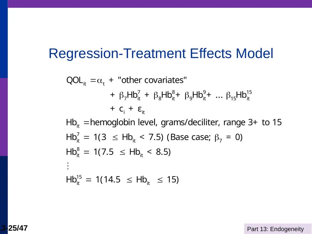
Regression-Treatment Effects Model<br>
24
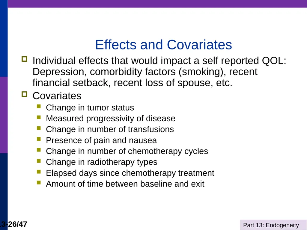
Effects and Covariates Individual effects that would impact a self reported QOL: Depression, comorbidity factors (smoking), recent financial setback, recent loss of spouse, etc.
Covariates
Change in tumor status
Measured progressivity of disease
Change in number of transfusions
Presence of pain and nausea
Change in number of chemotherapy cycles
Change in radiotherapy types
Elapsed days since chemotherapy treatment
Amount of time between baseline and exit<br>
Covariates
Change in tumor status
Measured progressivity of disease
Change in number of transfusions
Presence of pain and nausea
Change in number of chemotherapy cycles
Change in radiotherapy types
Elapsed days since chemotherapy treatment
Amount of time between baseline and exit<br>
25
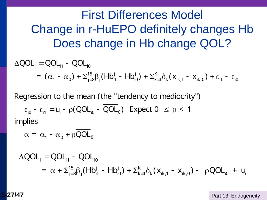
First Differences Model
Change in r-HuEPO definitely changes Hb
Does change in Hb change QOL?<br>
26
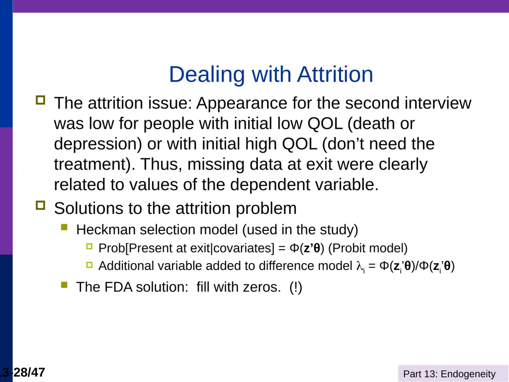
Dealing with Attrition The attrition issue: Appearance for the second interview was low for people with initial low QOL (death or depression) or with initial high QOL (don’t need the treatment). Thus, missing data at exit were clearly related to values of the dependent variable.
Solutions to the attrition problem
Heckman selection model (used in the study)
Prob[Present at exit|covariates] = Φ(z’θ) (Probit model)
Additional variable added to difference model i = Φ(zi’θ)/Φ(zi’θ)
The FDA solution: fill with zeros. (!)<br>
Solutions to the attrition problem
Heckman selection model (used in the study)
Prob[Present at exit|covariates] = Φ(z’θ) (Probit model)
Additional variable added to difference model i = Φ(zi’θ)/Φ(zi’θ)
The FDA solution: fill with zeros. (!)<br>
27
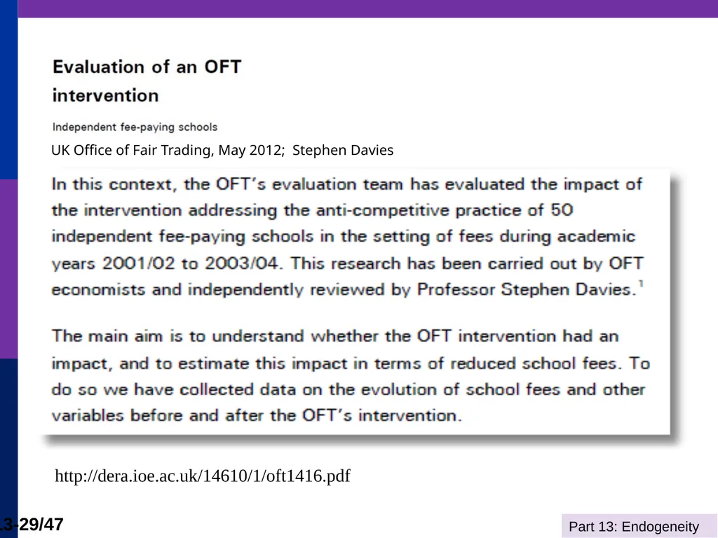
UK Office of Fair Trading, May 2012; Stephen Davies http://dera.ioe.ac.uk/14610/1/oft1416.pdf<br>
28
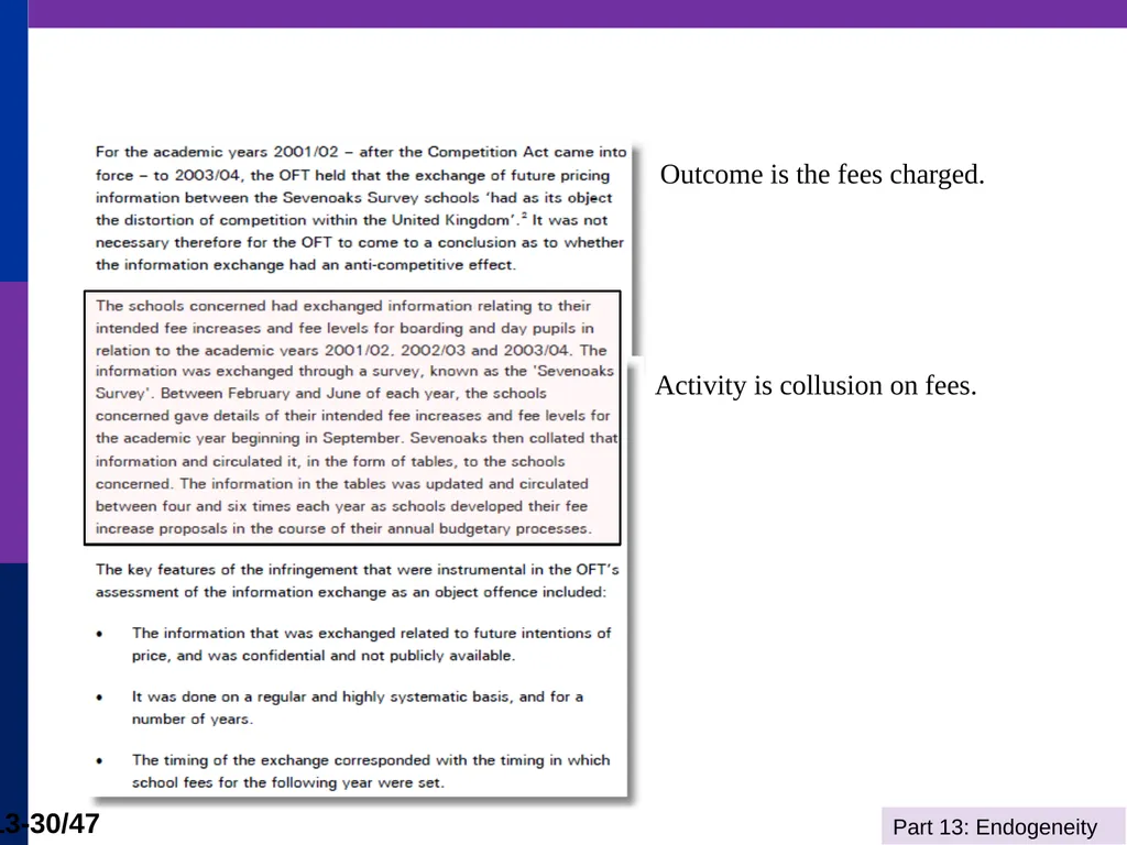
Outcome is the fees charged. Activity is collusion on fees.<br>
29
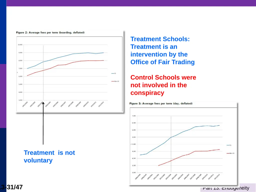
Treatment Schools: Treatment is an intervention by the Office of Fair Trading
Control Schools were not involved in the conspiracy Treatment is not voluntary<br>
Control Schools were not involved in the conspiracy Treatment is not voluntary<br>
30
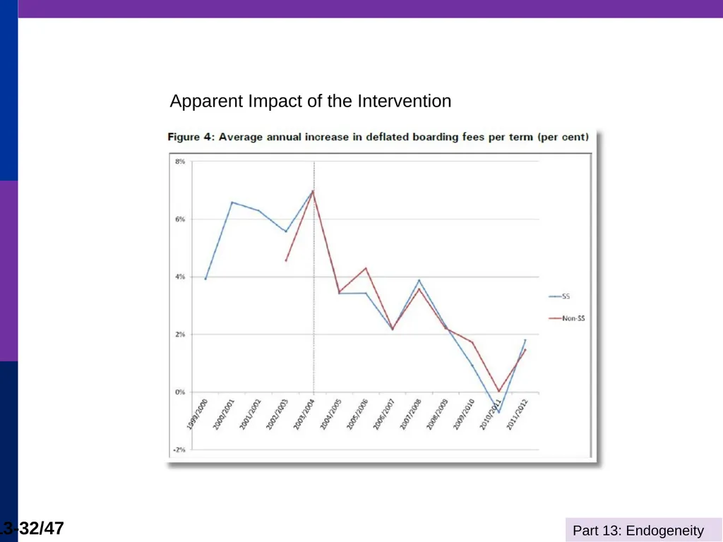
Apparent Impact of the Intervention<br>
31
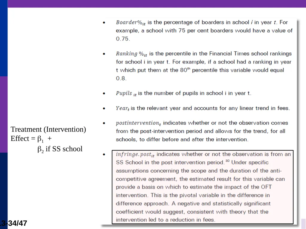
Treatment (Intervention) Effect = 1 +
2 if SS school<br>
2 if SS school<br>
32
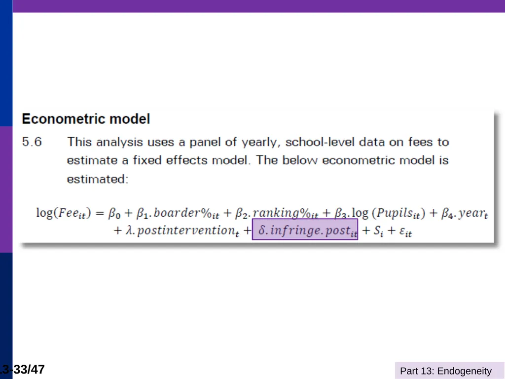
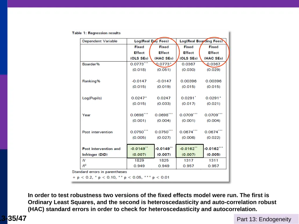
In order to test robustness two versions of the fixed effects model were run. The first is Ordinary Least Squares, and the second is heteroscedasticity and auto-correlation robust (HAC) standard errors in order to check for heteroscedasticity and autocorrelation.<br>
33
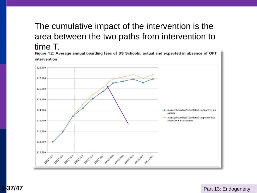
The cumulative impact of the intervention is the area between the two paths from intervention to time T.<br>
34
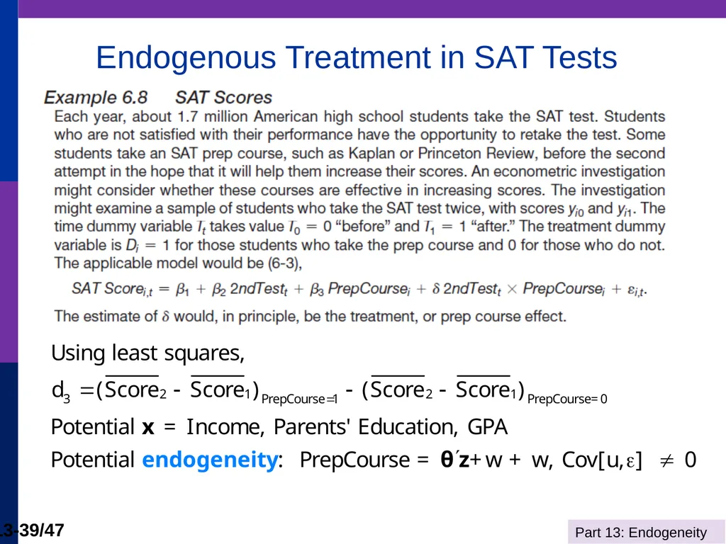
Endogenous Treatment in SAT Tests<br>
35
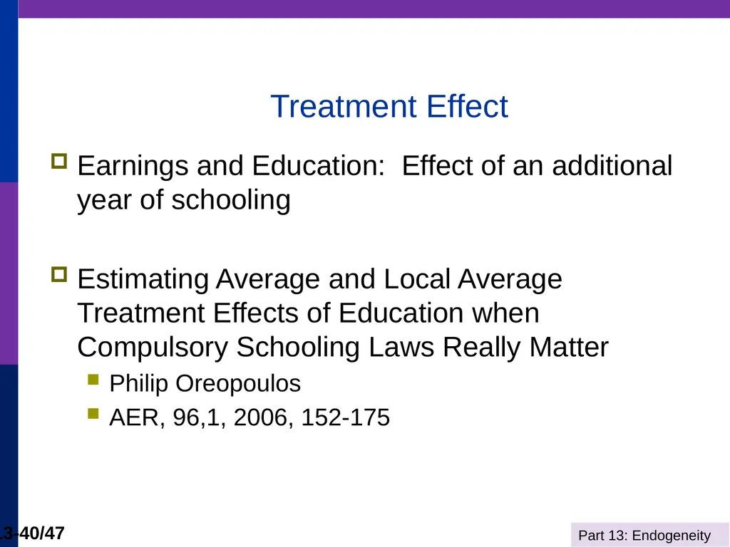
Treatment Effect Earnings and Education: Effect of an additional year of schooling
Estimating Average and Local Average Treatment Effects of Education when Compulsory Schooling Laws Really Matter
Philip Oreopoulos
AER, 96,1, 2006, 152-175<br>
Estimating Average and Local Average Treatment Effects of Education when Compulsory Schooling Laws Really Matter
Philip Oreopoulos
AER, 96,1, 2006, 152-175<br>
36
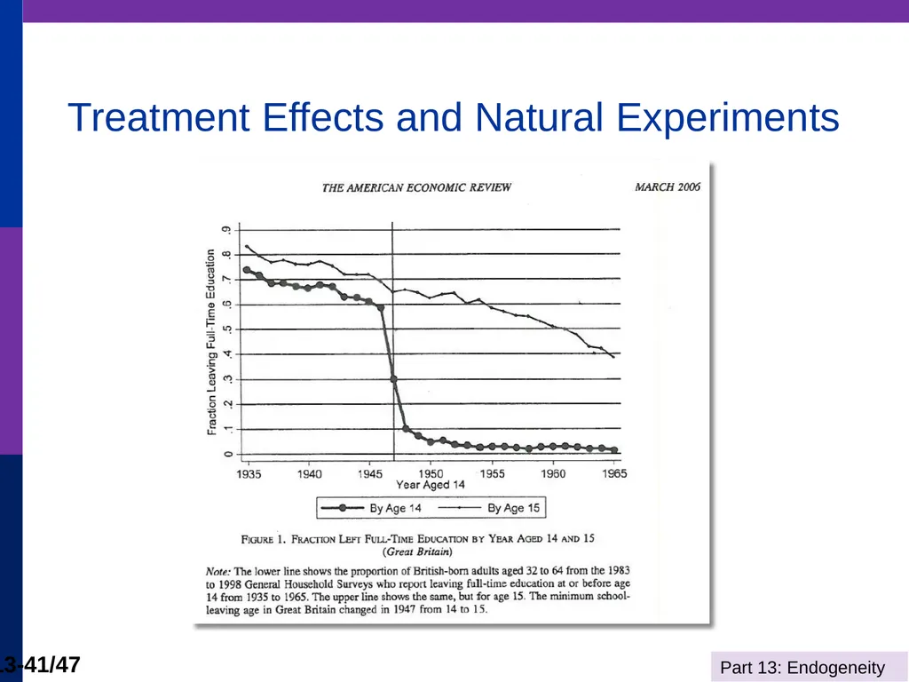
Treatment Effects and Natural Experiments<br>
37
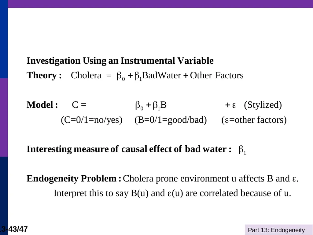
The First IV Study Was a Natural Experiment
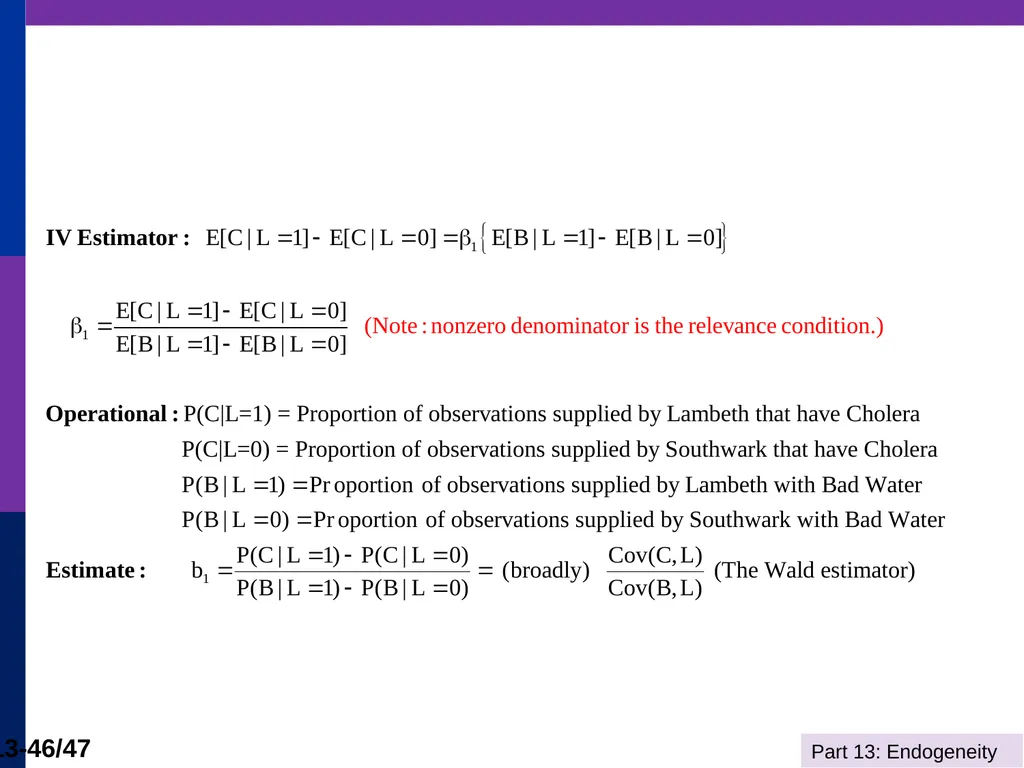
(Snow, J., On the Mode of Communication of Cholera, 1855)
http://www.ph.ucla.edu/epi/snow/snowbook3.html London Cholera epidemic, ca 1853-4
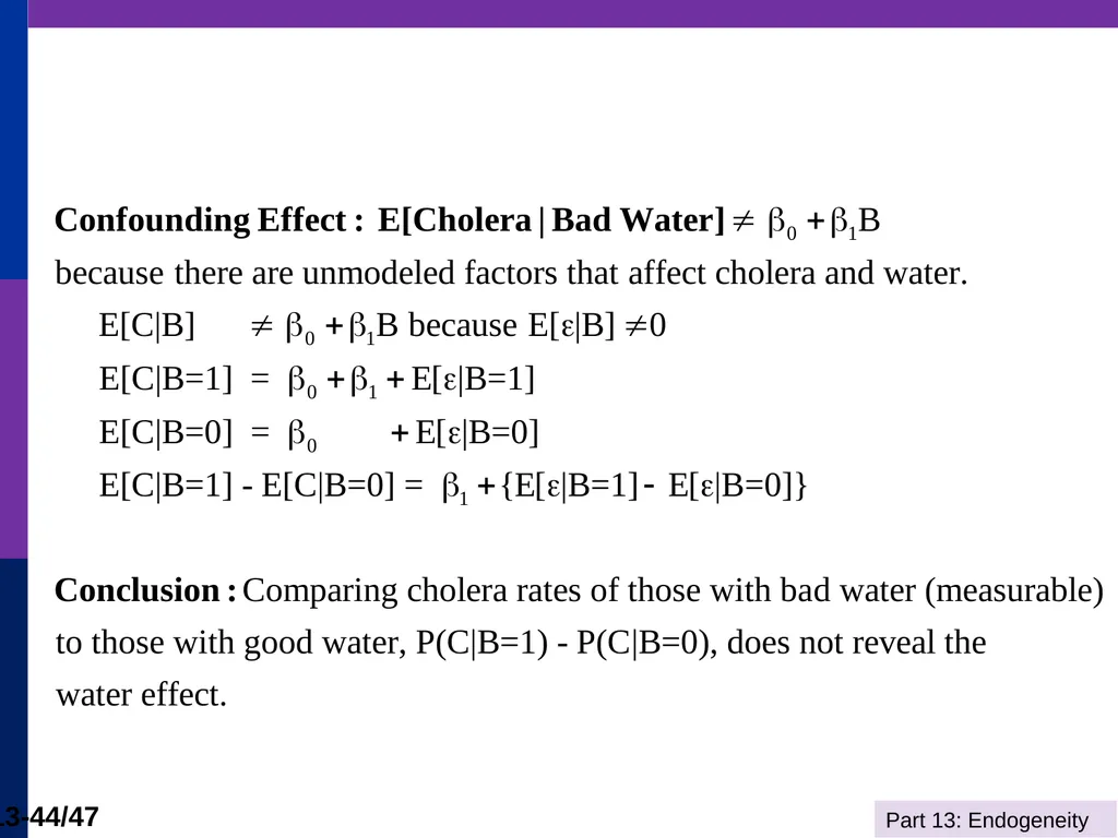
Cholera = f(Water Purity,u) + ε.
‘Causal’ effect of water purity on cholera?
Purity=f(cholera prone environment (poor, garbage in streets, rodents, etc.). Regression does not work.
Two London water companies
Lambeth Southwark & Vauxhall
Main sewage discharge Paul Grootendorst: A Review of Instrumental Variables Estimation of Treatment Effects… http://individual.utoronto.ca/grootendorst/pdf/IV_Paper_Sept6_2007.pdf
A review of instrumental variables estimation in the applied health sciences. Health Services and Outcomes Research Methodology 2007; 7(3-4):159-179. River Thames<br>
Cholera = f(Water Purity,u) + ε.
‘Causal’ effect of water purity on cholera?
Purity=f(cholera prone environment (poor, garbage in streets, rodents, etc.). Regression does not work.
Two London water companies
Lambeth Southwark & Vauxhall
Main sewage discharge Paul Grootendorst: A Review of Instrumental Variables Estimation of Treatment Effects… http://individual.utoronto.ca/grootendorst/pdf/IV_Paper_Sept6_2007.pdf
A review of instrumental variables estimation in the applied health sciences. Health Services and Outcomes Research Methodology 2007; 7(3-4):159-179. River Thames<br>
38
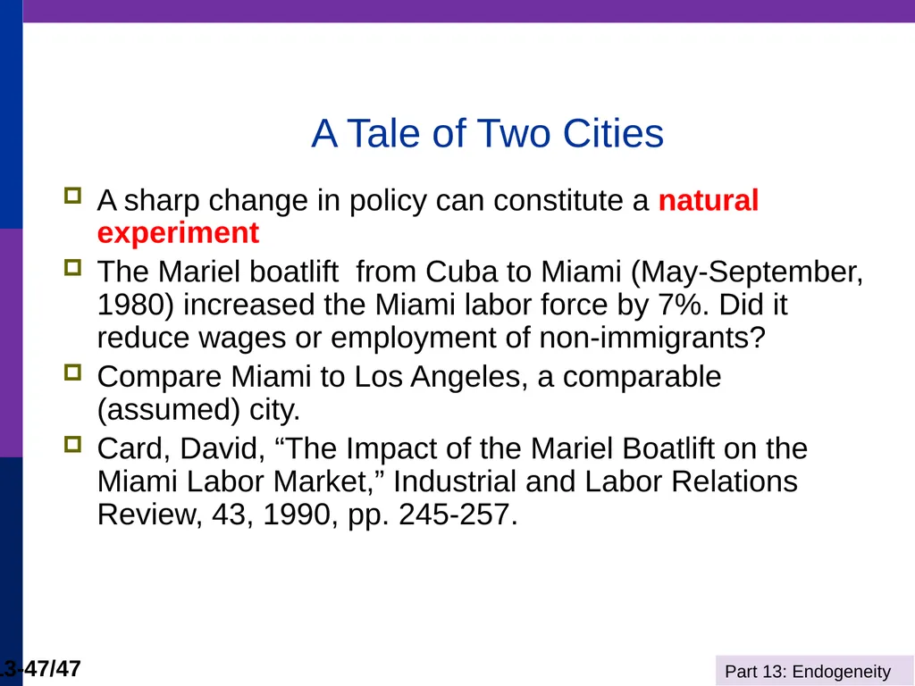
A Tale of Two Cities A sharp change in policy can constitute a natural experiment
The Mariel boatlift from Cuba to Miami (May-September, 1980) increased the Miami labor force by 7%. Did it reduce wages or employment of non-immigrants?
Compare Miami to Los Angeles, a comparable (assumed) city.
Card, David, “The Impact of the Mariel Boatlift on the Miami Labor Market,” Industrial and Labor Relations Review, 43, 1990, pp. 245-257.<br>
The Mariel boatlift from Cuba to Miami (May-September, 1980) increased the Miami labor force by 7%. Did it reduce wages or employment of non-immigrants?
Compare Miami to Los Angeles, a comparable (assumed) city.
Card, David, “The Impact of the Mariel Boatlift on the Miami Labor Market,” Industrial and Labor Relations Review, 43, 1990, pp. 245-257.<br>
39
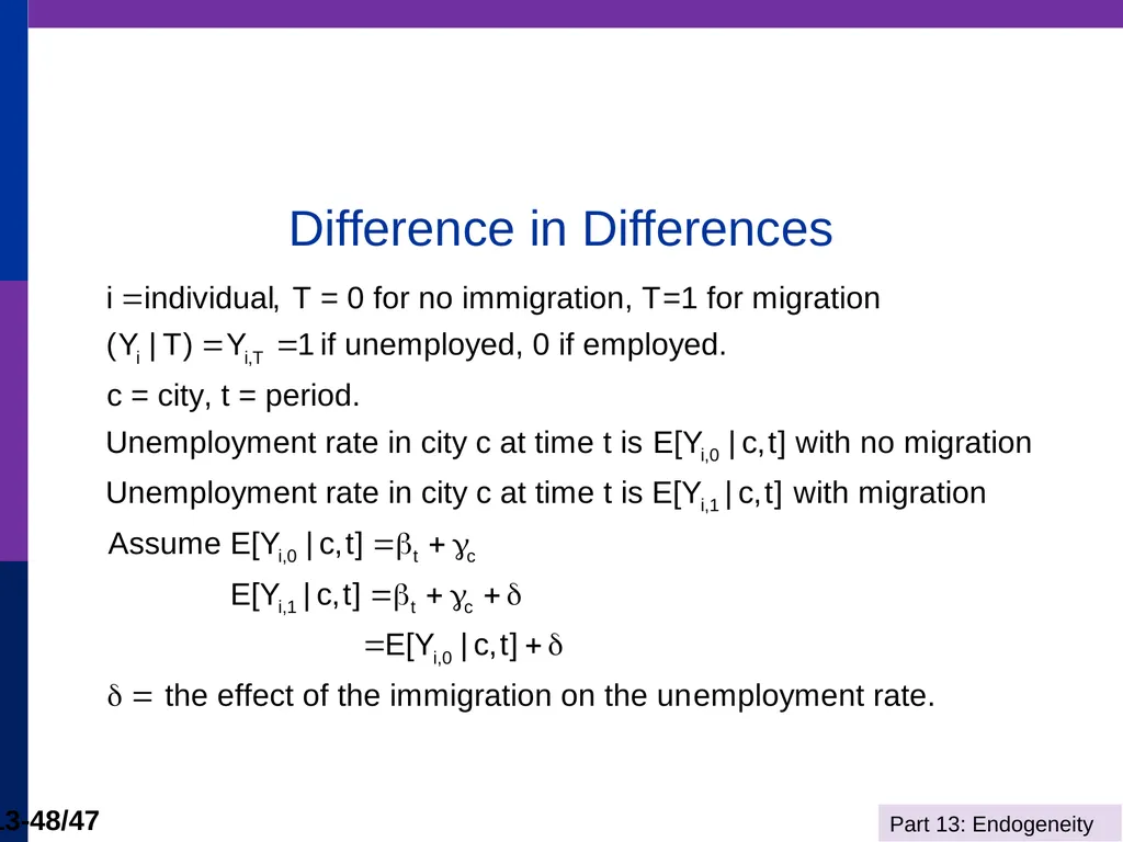
Difference in Differences<br>
40
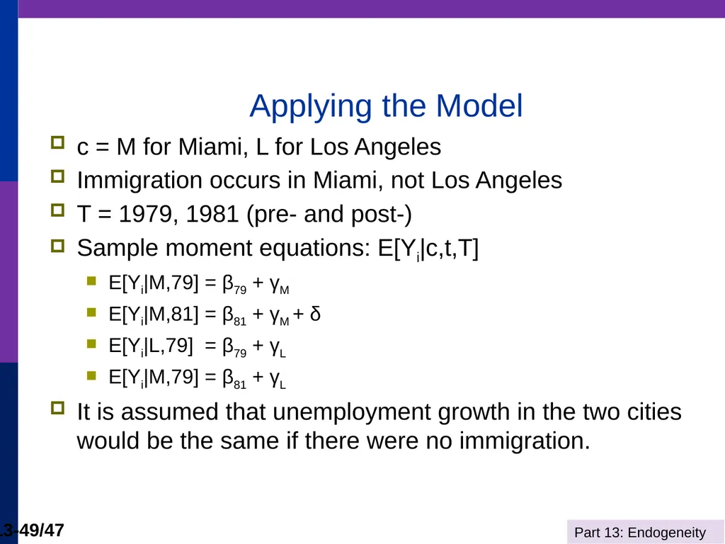
Applying the Model c = M for Miami, L for Los Angeles
Immigration occurs in Miami, not Los Angeles
T = 1979, 1981 (pre- and post-)
Sample moment equations: E[Yi|c,t,T]
E[Yi|M,79] = β79 + γM
E[Yi|M,81] = β81 + γM + δ
E[Yi|L,79] = β79 + γL
E[Yi|M,79] = β81 + γL
It is assumed that unemployment growth in the two cities would be the same if there were no immigration.<br>
Immigration occurs in Miami, not Los Angeles
T = 1979, 1981 (pre- and post-)
Sample moment equations: E[Yi|c,t,T]
E[Yi|M,79] = β79 + γM
E[Yi|M,81] = β81 + γM + δ
E[Yi|L,79] = β79 + γL
E[Yi|M,79] = β81 + γL
It is assumed that unemployment growth in the two cities would be the same if there were no immigration.<br>
41
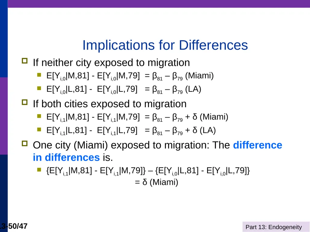
Implications for Differences If neither city exposed to migration
E[Yi,0|M,81] - E[Yi,0|M,79] = β81 – β79 (Miami)
E[Yi,0|L,81] - E[Yi,0|L,79] = β81 – β79 (LA)
If both cities exposed to migration
E[Yi,1|M,81] - E[Yi,1|M,79] = β81 – β79 + δ (Miami)
E[Yi,1|L,81] - E[Yi,1|L,79] = β81 – β79 + δ (LA)
One city (Miami) exposed to migration: The difference in differences is.
{E[Yi,1|M,81] - E[Yi,1|M,79]} – {E[Yi,0|L,81] - E[Yi,0|L,79]} = δ (Miami)<br>
E[Yi,0|M,81] - E[Yi,0|M,79] = β81 – β79 (Miami)
E[Yi,0|L,81] - E[Yi,0|L,79] = β81 – β79 (LA)
If both cities exposed to migration
E[Yi,1|M,81] - E[Yi,1|M,79] = β81 – β79 + δ (Miami)
E[Yi,1|L,81] - E[Yi,1|L,79] = β81 – β79 + δ (LA)
One city (Miami) exposed to migration: The difference in differences is.
{E[Yi,1|M,81] - E[Yi,1|M,79]} – {E[Yi,0|L,81] - E[Yi,0|L,79]} = δ (Miami)<br>
42
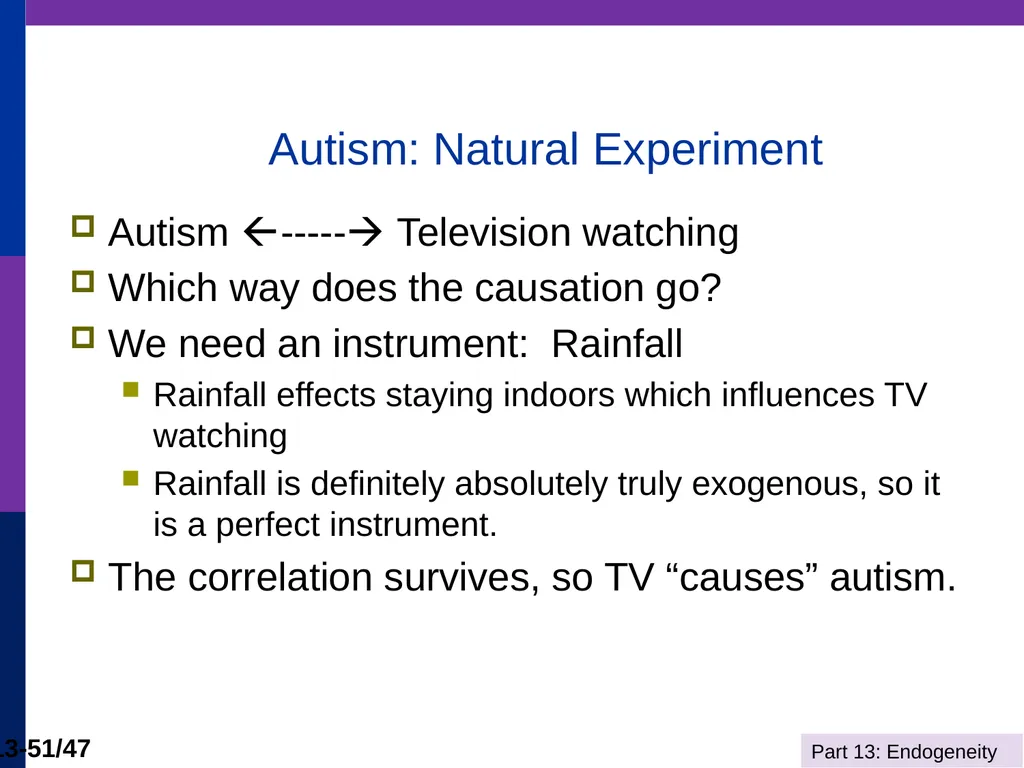
Autism: Natural Experiment Autism ----- Television watching
Which way does the causation go?
We need an instrument: Rainfall
Rainfall effects staying indoors which influences TV watching
Rainfall is definitely absolutely truly exogenous, so it is a perfect instrument.
The correlation survives, so TV “causes” autism.<br>
Which way does the causation go?
We need an instrument: Rainfall
Rainfall effects staying indoors which influences TV watching
Rainfall is definitely absolutely truly exogenous, so it is a perfect instrument.
The correlation survives, so TV “causes” autism.<br>