
Energy-Aware Wireless Scheduling with Near Optimal
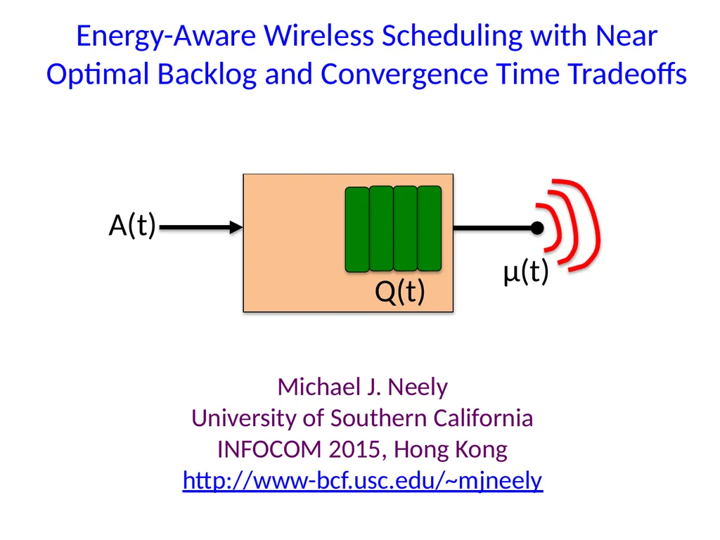
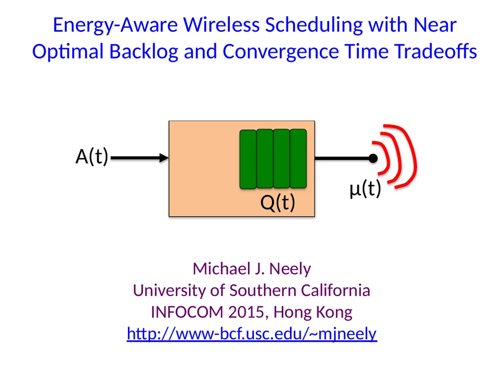
Description: Energy-Aware Wireless Scheduling with Near Optimal Backlog and Convergence Time Tradeoffs Michael J. Neely University of Southern California INFOCOM 2015, Hong Kong http:www-bcf.usc.edumjneely A(t) Q(t) μ(t) A(t) Q(t) μ(t) Q(t1)
Related Topics
Download Presentation
"Energy-Aware Wireless Scheduling with Near Optimal" is the property of its rightful owner. Permission is granted to download and print the materials on this website for personal, non-commercial use only, and to display it on your personal computer provided you do not modify the materials and that you retain all copyright notices contained in the materials. By downloading content from our website, you accept the terms of this agreement.
Presentation Transcript
slide1. Energy-Aware Wireless Scheduling with Near Optimal Backlog and Convergence Time Tradeoffs Michael J. Neely
University of Southern California
INFOCOM 2015, Hong Kong
http://www-bcf.usc.edu/~mjneely A(t) Q(t) μ(t)<br>
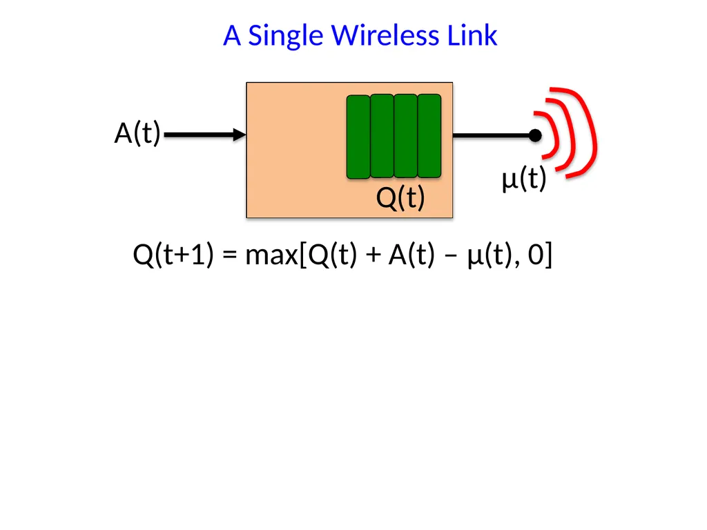
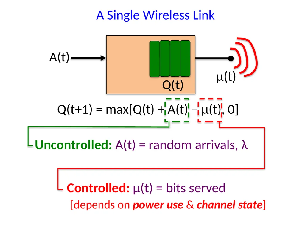
slide2. A(t) Q(t) μ(t) Q(t+1) = max[Q(t) + A(t) – μ(t), 0] A Single Wireless Link<br>
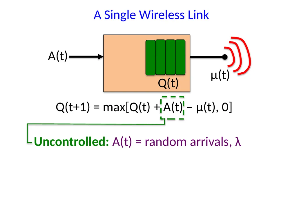
slide3. A(t) Q(t) μ(t) Q(t+1) = max[Q(t) + A(t) – μ(t), 0] A Single Wireless Link Uncontrolled: A(t) = random arrivals, λ<br>
slide4. A(t) Q(t) μ(t) Q(t+1) = max[Q(t) + A(t) – μ(t), 0] A Single Wireless Link Uncontrolled: A(t) = random arrivals, λ Controlled: μ(t) = bits served
[depends on power use & channel state]<br>
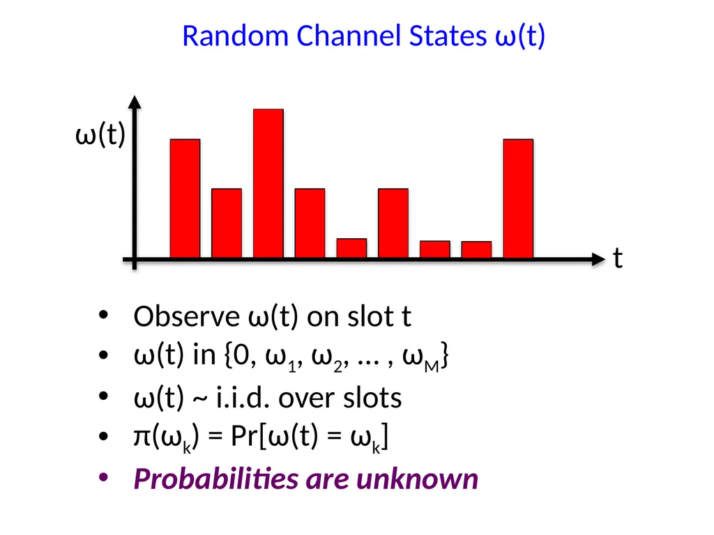
slide5. Random Channel States ω(t) Observe ω(t) on slot t
ω(t) in {0, ω1, ω2, … , ωM}
ω(t) ~ i.i.d. over slots
π(ωk) = Pr[ω(t) = ωk]
Probabilities are unknown<br>
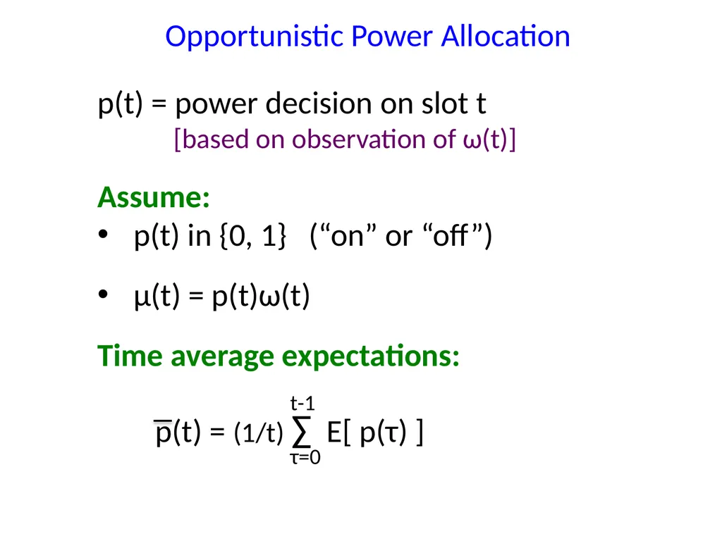
slide6. Opportunistic Power Allocation p(t) = power decision on slot t
[based on observation of ω(t)]
Assume:
p(t) in {0, 1} (“on” or “off”)
μ(t) = p(t)ω(t)
Time average expectations:
p(t) = (1/t) ∑ E[ p(τ) ] τ=0 t-1<br>
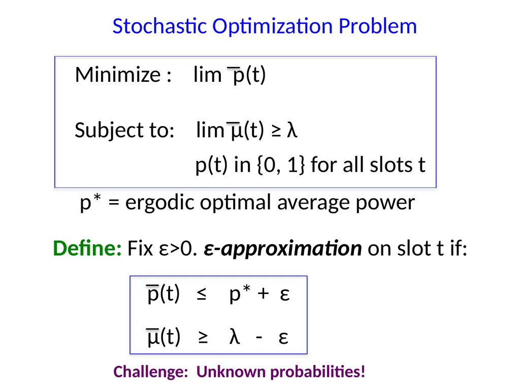
slide7. Stochastic Optimization Problem Minimize : lim p(t)
Subject to: lim μ(t) ≥ λ
p(t) in {0, 1} for all slots t p* = ergodic optimal average power Define: Fix ε>0. ε-approximation on slot t if:
p(t) ≤ p* + ε
μ(t) ≥ λ - ε Challenge: Unknown probabilities!<br>
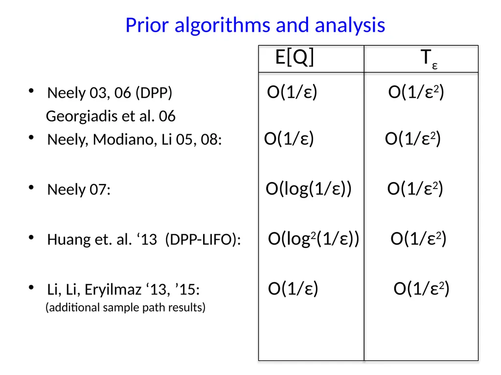
slide8. Prior algorithms and analysis E[Q] Tε
Neely 03, 06 (DPP) O(1/ε) O(1/ε2)
Georgiadis et al. 06
Neely, Modiano, Li 05, 08: O(1/ε) O(1/ε2)
Neely 07: O(log(1/ε)) O(1/ε2)
Huang et. al. ‘13 (DPP-LIFO): O(log2(1/ε)) O(1/ε2)
Li, Li, Eryilmaz ‘13, ’15: O(1/ε) O(1/ε2)
(additional sample path results)<br>
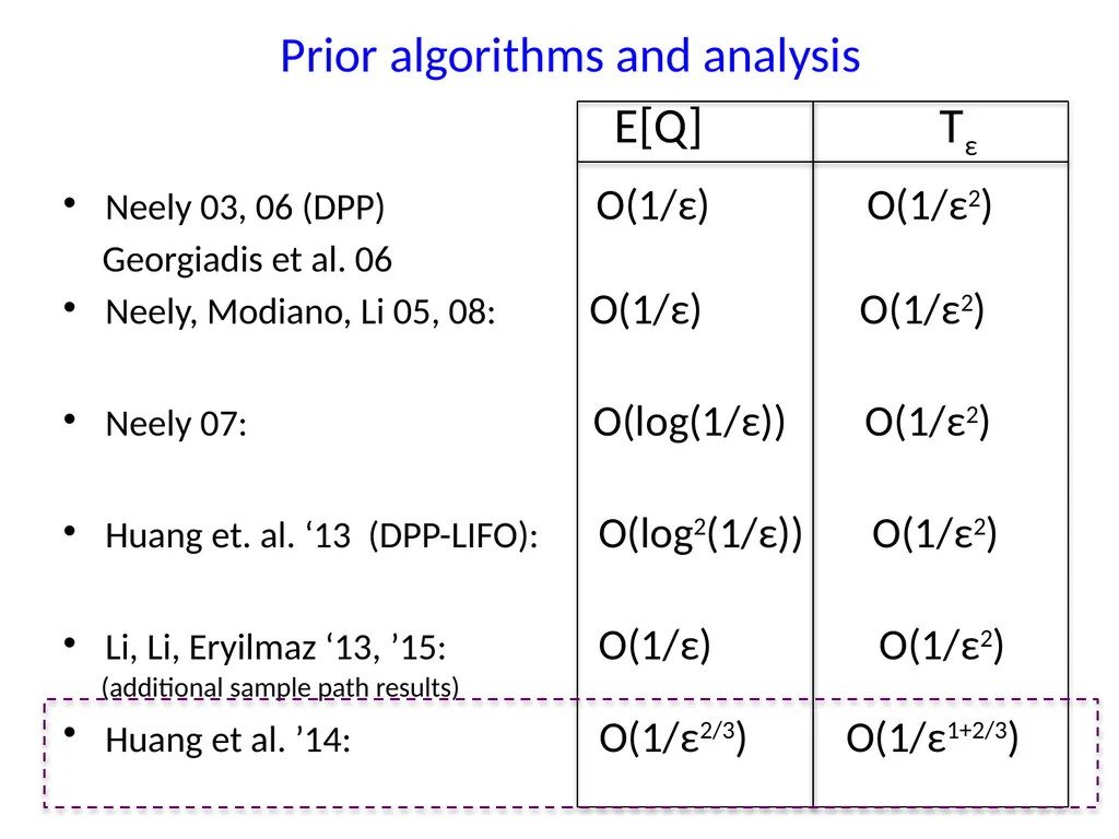
slide9. Prior algorithms and analysis E[Q] Tε
Neely 03, 06 (DPP) O(1/ε) O(1/ε2)
Georgiadis et al. 06
Neely, Modiano, Li 05, 08: O(1/ε) O(1/ε2)
Neely 07: O(log(1/ε)) O(1/ε2)
Huang et. al. ‘13 (DPP-LIFO): O(log2(1/ε)) O(1/ε2)
Li, Li, Eryilmaz ‘13, ’15: O(1/ε) O(1/ε2)
(additional sample path results)
Huang et al. ’14: O(1/ε2/3) O(1/ε1+2/3)<br>
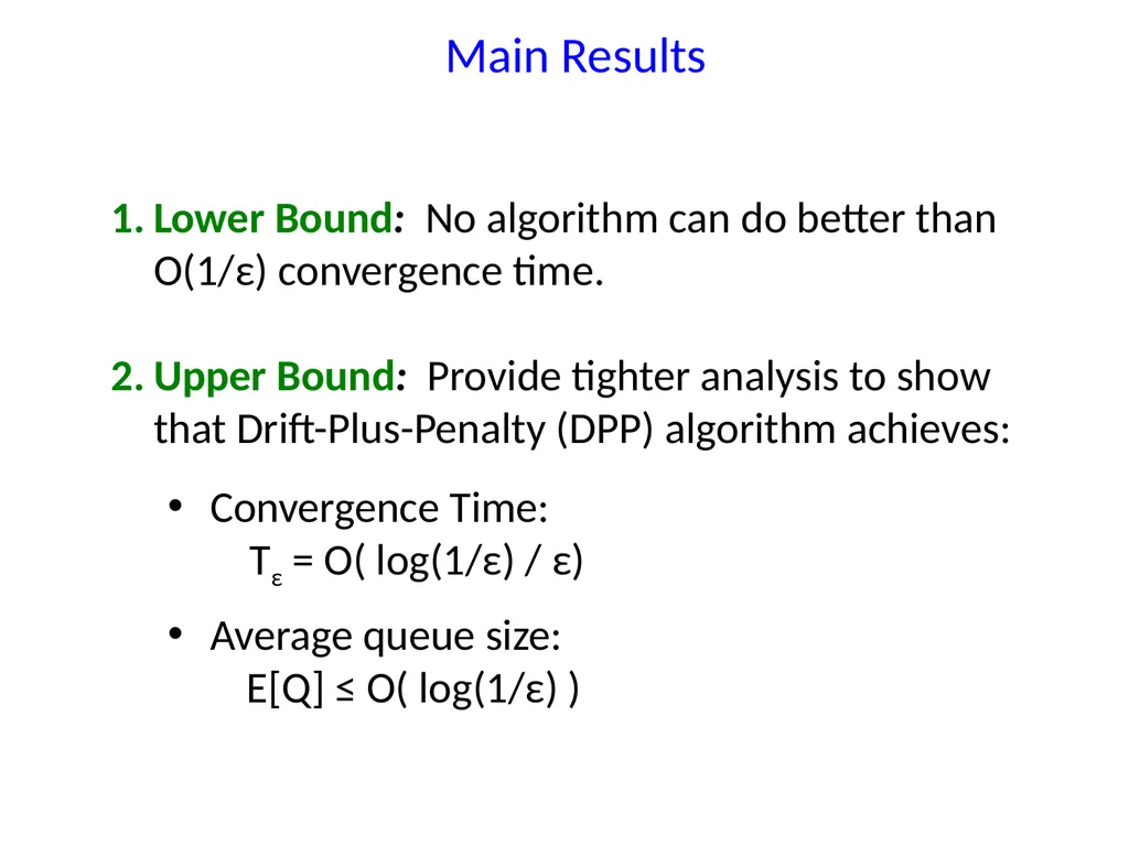
slide10. Main Results Lower Bound: No algorithm can do better than O(1/ε) convergence time.
Upper Bound: Provide tighter analysis to show that Drift-Plus-Penalty (DPP) algorithm achieves:
Convergence Time: Tε = O( log(1/ε) / ε)
Average queue size:
E[Q] ≤ O( log(1/ε) )<br>
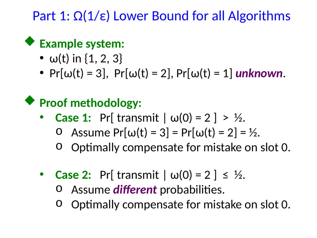
slide11. Part 1: Ω(1/ε) Lower Bound for all Algorithms Example system:
ω(t) in {1, 2, 3}
Pr[ω(t) = 3], Pr[ω(t) = 2], Pr[ω(t) = 1] unknown.
Proof methodology:
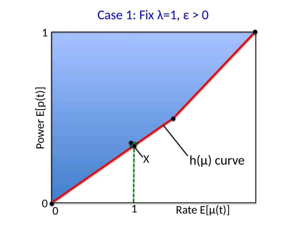
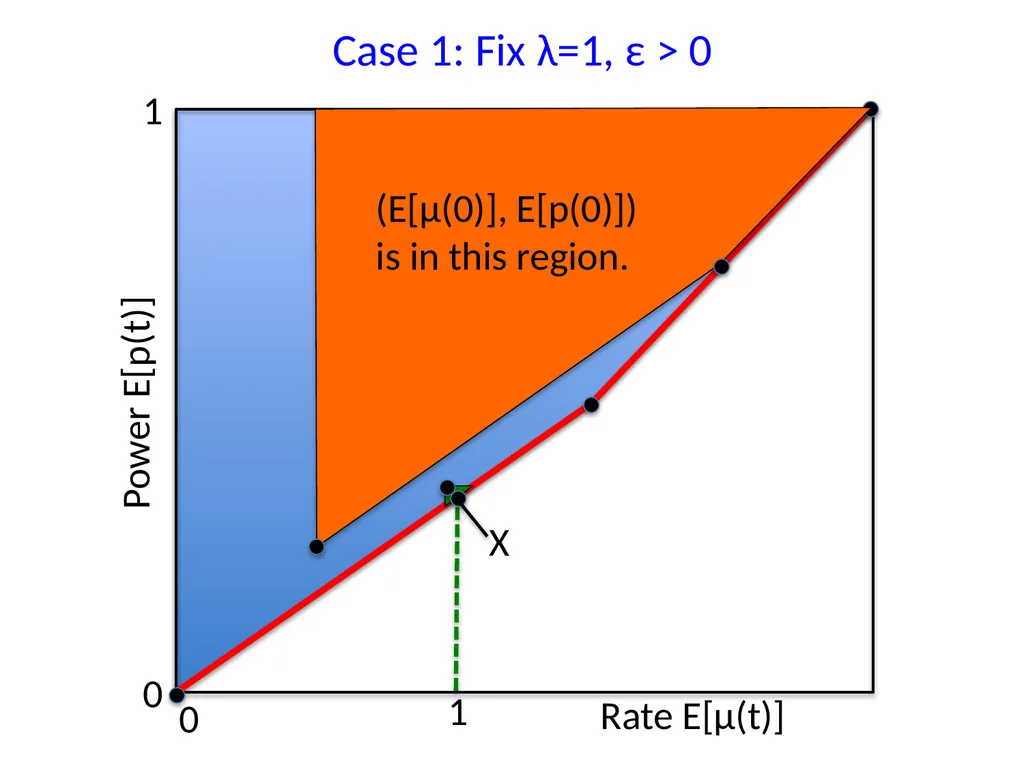
Case 1: Pr[ transmit | ω(0) = 2 ] > ½.
Assume Pr[ω(t) = 3] = Pr[ω(t) = 2] = ½.
Optimally compensate for mistake on slot 0.
Case 2: Pr[ transmit | ω(0) = 2 ] ≤ ½.
Assume different probabilities.
Optimally compensate for mistake on slot 0.<br>
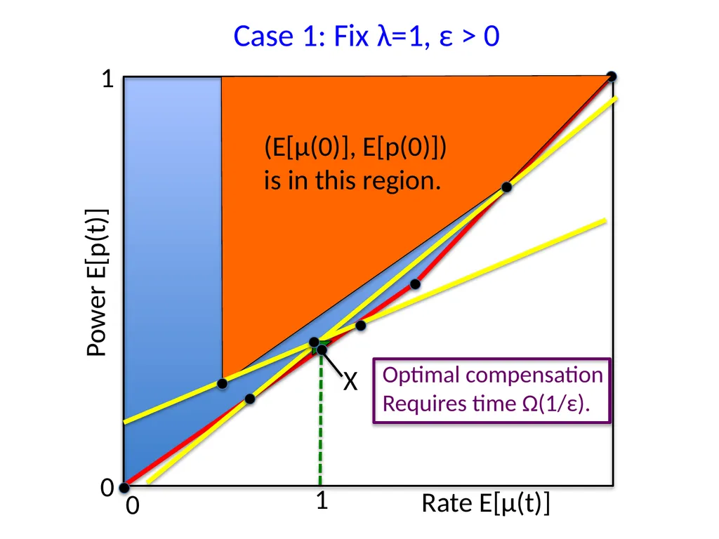
slide12. Case 1: Fix λ=1, ε > 0 Rate E[μ(t)] Power E[p(t)] X 1 0 0 1 h(μ) curve<br>
slide13. Case 1: Fix λ=1, ε > 0 Rate E[μ(t)] Power E[p(t)] A X 1 0 0 1 (E[μ(0)], E[p(0)])
is in this region.<br>
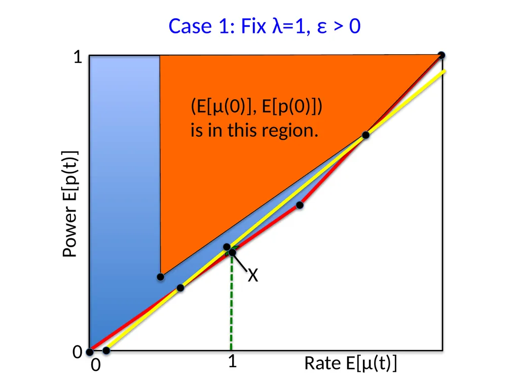
slide14. Case 1: Fix λ=1, ε > 0 Rate E[μ(t)] Power E[p(t)] A X 1 0 0 1 (E[μ(0)], E[p(0)])
is in this region.<br>
slide15. Case 1: Fix λ=1, ε > 0 Rate E[μ(t)] Power E[p(t)] A X 1 0 0 1 (E[μ(0)], E[p(0)])
is in this region.<br>
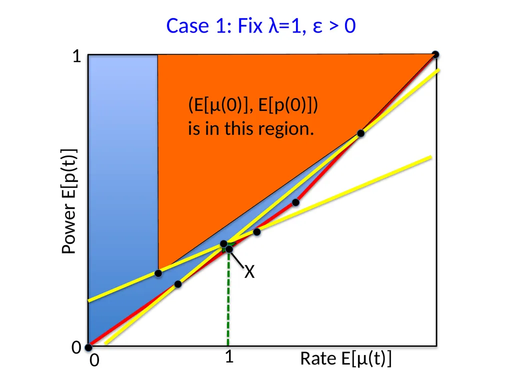
slide16. Case 1: Fix λ=1, ε > 0 Rate E[μ(t)] Power E[p(t)] A 1 0 0 1 (E[μ(0)], E[p(0)])
is in this region. X Optimal compensation
Requires time Ω(1/ε).<br>
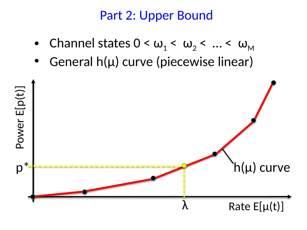
slide17. Part 2: Upper Bound Channel states 0 < ω1 < ω2 < … < ωM
General h(μ) curve (piecewise linear) Power E[p(t)] Rate E[μ(t)] λ h(μ) curve p*<br>
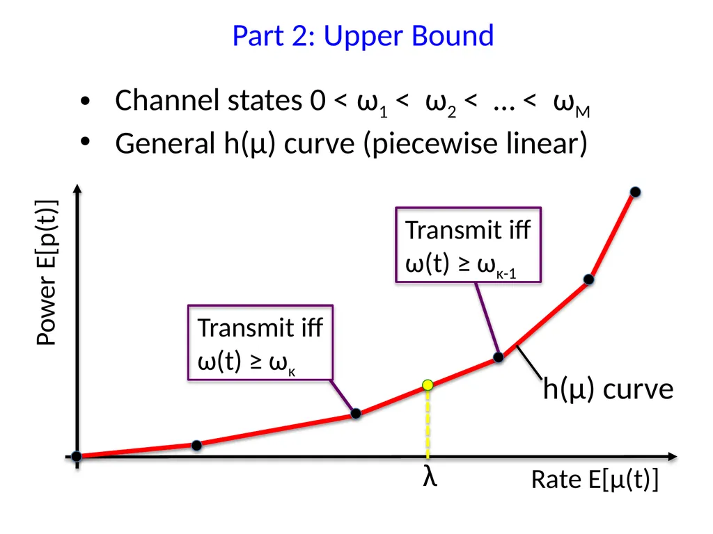
slide18. Part 2: Upper Bound Channel states 0 < ω1 < ω2 < … < ωM
General h(μ) curve (piecewise linear) Rate E[μ(t)] λ h(μ) curve Transmit iff
ω(t) ≥ ωκ-1 Transmit iff
ω(t) ≥ ωκ Power E[p(t)]<br>
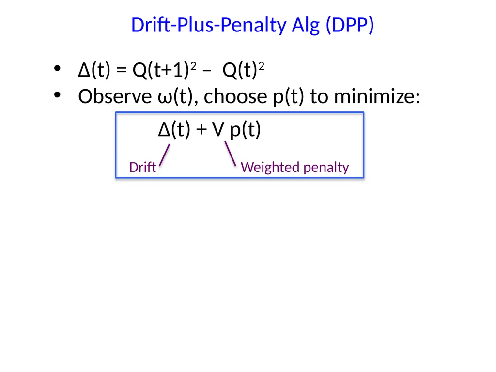
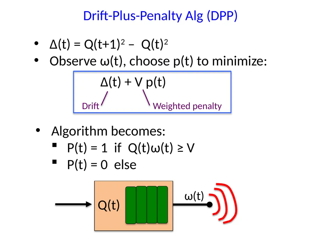
slide19. Drift-Plus-Penalty Alg (DPP) Δ(t) = Q(t+1)2 – Q(t)2
Observe ω(t), choose p(t) to minimize:
Δ(t) + V p(t) Weighted penalty Drift<br>
slide20. Drift-Plus-Penalty Alg (DPP) Δ(t) = Q(t+1)2 – Q(t)2
Observe ω(t), choose p(t) to minimize:
Δ(t) + V p(t) Weighted penalty Drift Algorithm becomes:
P(t) = 1 if Q(t)ω(t) ≥ V
P(t) = 0 else Q(t) ω(t)<br>
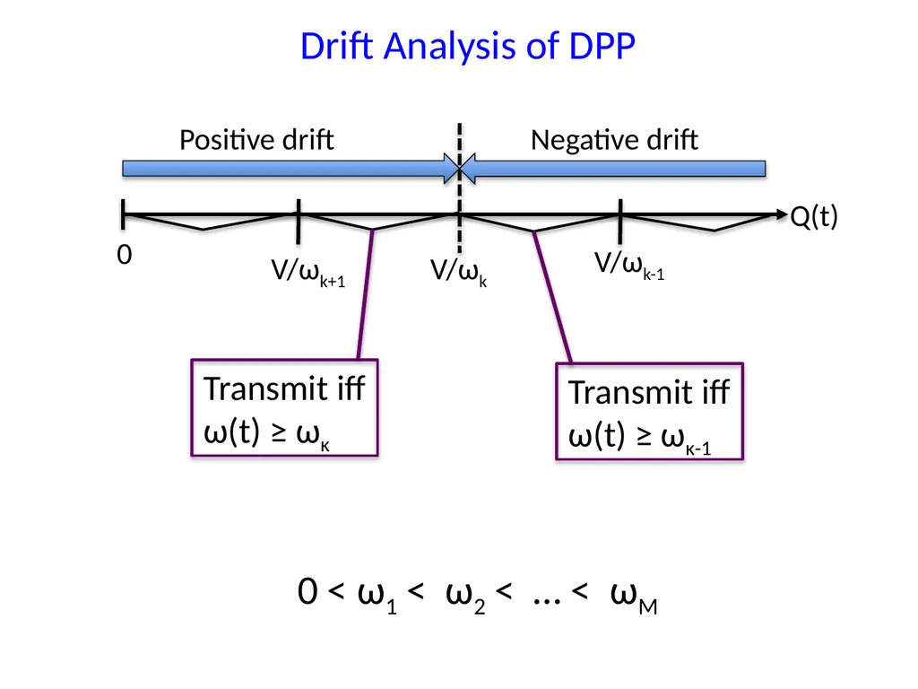
slide21. Drift Analysis of DPP V/ωk V/ωk+1 V/ωk-1 0 Q(t) Positive drift Negative drift 0 < ω1 < ω2 < … < ωM<br>
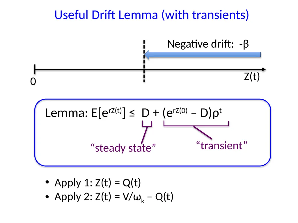
slide22. Useful Drift Lemma (with transients) Z(t) Negative drift: -β 0 Lemma: E[erZ(t)] ≤ D + (erZ(0) – D)ρt “steady state” “transient” Apply 1: Z(t) = Q(t)
Apply 2: Z(t) = V/ωk – Q(t)<br>
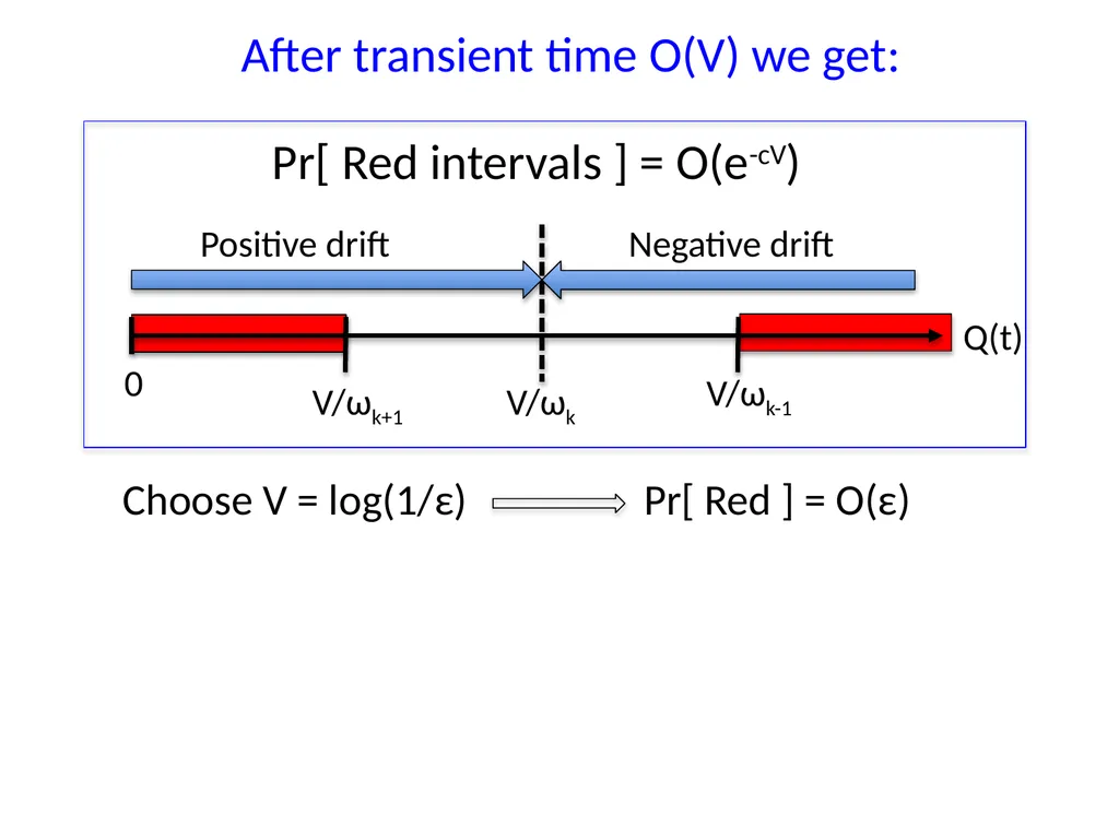
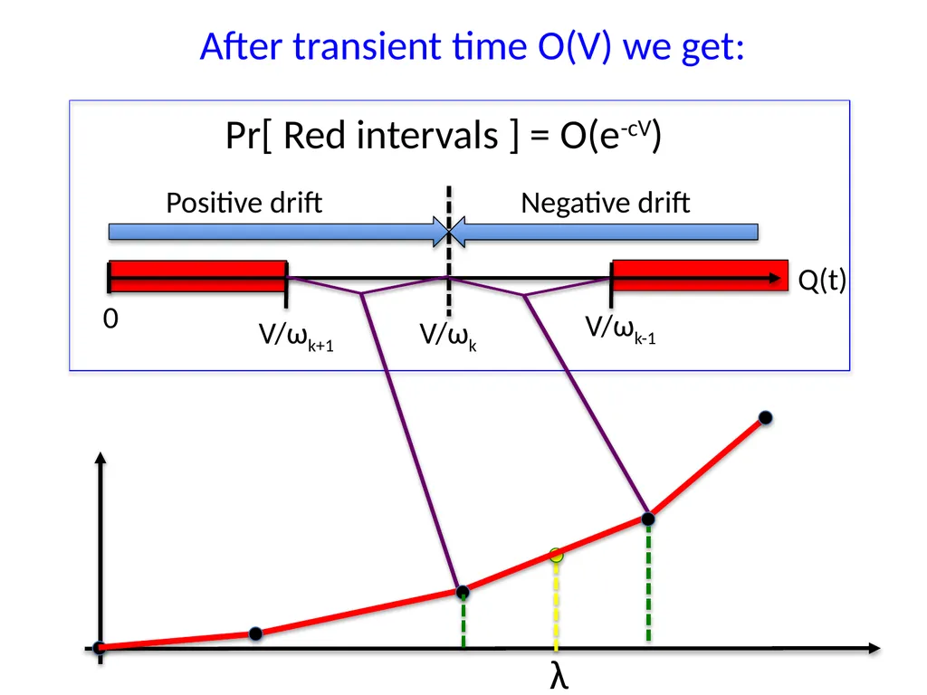
slide23. After transient time O(V) we get: V/ωk V/ωk+1 V/ωk-1 0 Q(t) Positive drift Negative drift Pr[ Red intervals ] = O(e-cV) Choose V = log(1/ε) Pr[ Red ] = O(ε)<br>
slide24. After transient time O(V) we get: V/ωk V/ωk+1 V/ωk-1 0 Q(t) Positive drift Negative drift Pr[ Red intervals ] = O(e-cV) λ<br>
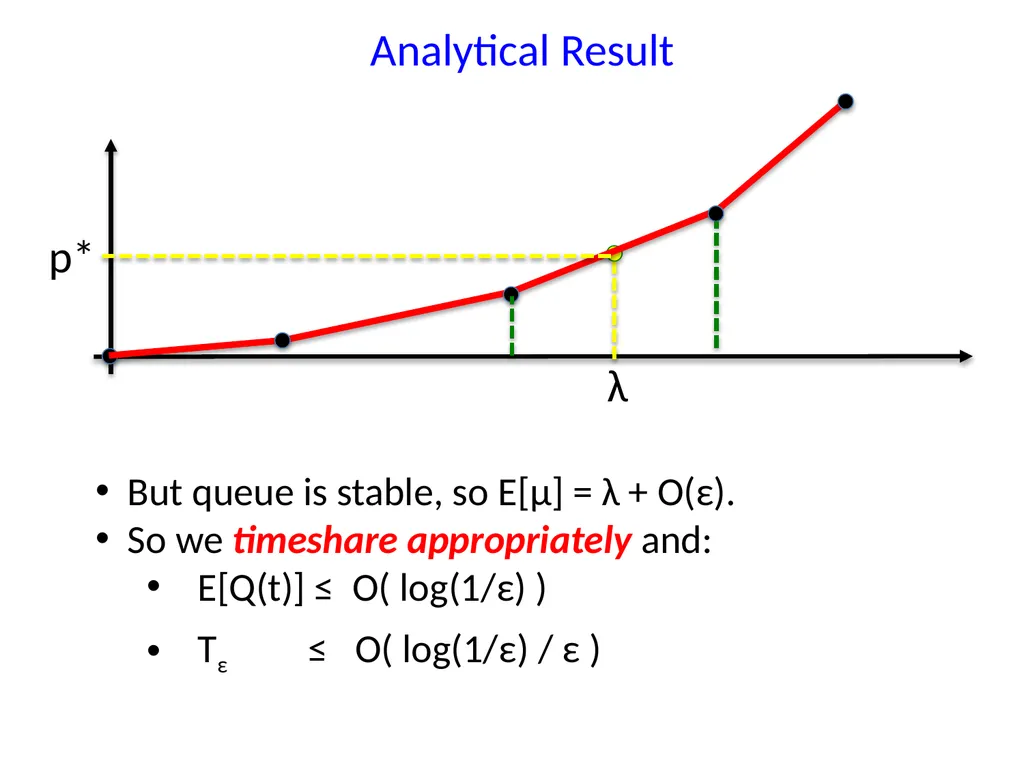
slide25. Analytical Result λ But queue is stable, so E[μ] = λ + O(ε).
So we timeshare appropriately and:
E[Q(t)] ≤ O( log(1/ε) )
Tε ≤ O( log(1/ε) / ε ) p*<br>
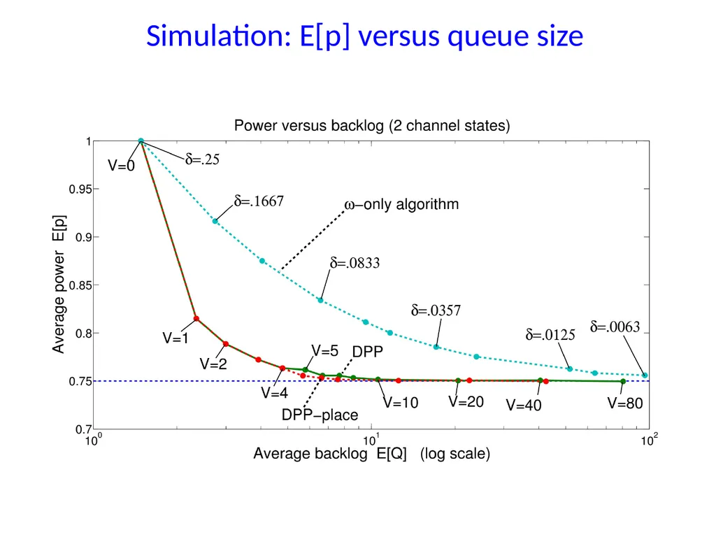
slide26. Simulation: E[p] versus queue size<br>
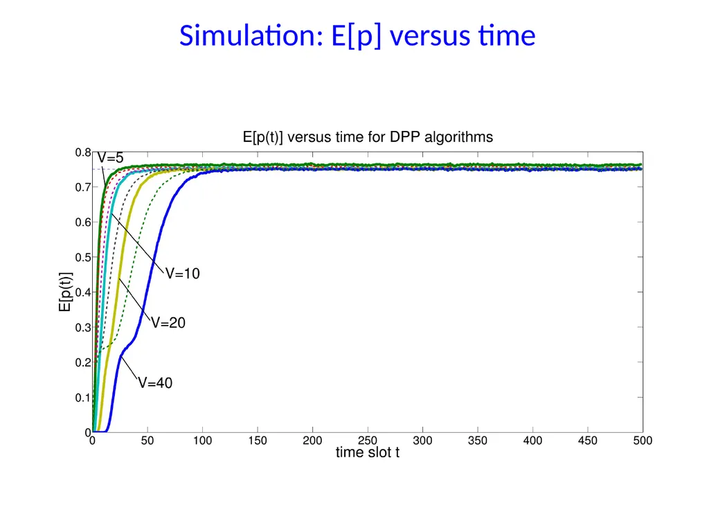
slide27. Simulation: E[p] versus time<br>
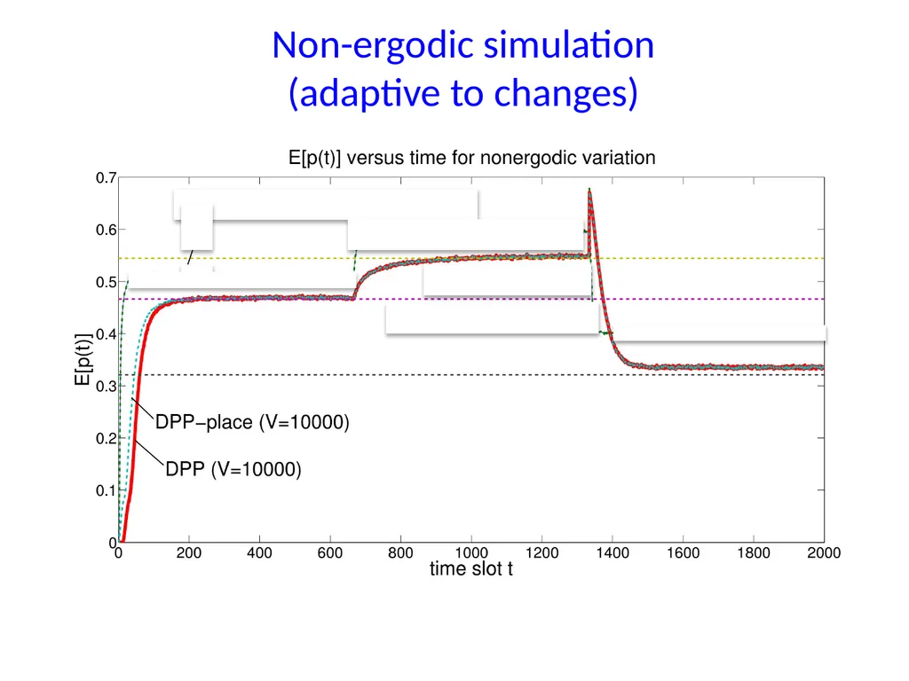
slide28. Non-ergodic simulation
(adaptive to changes)<br>
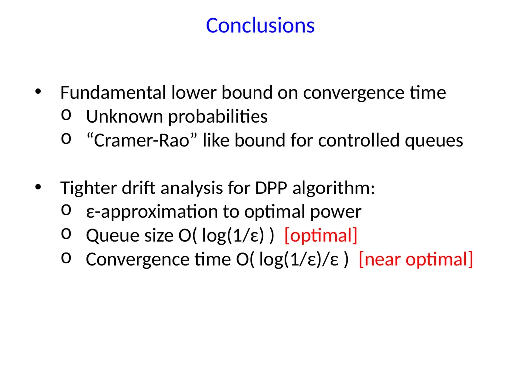
slide29. Conclusions Fundamental lower bound on convergence time
Unknown probabilities
“Cramer-Rao” like bound for controlled queues
Tighter drift analysis for DPP algorithm:
ε-approximation to optimal power
Queue size O( log(1/ε) ) [optimal]
Convergence time O( log(1/ε)/ε ) [near optimal]<br>
University of Southern California
INFOCOM 2015, Hong Kong
http://www-bcf.usc.edu/~mjneely A(t) Q(t) μ(t)<br>
slide2. A(t) Q(t) μ(t) Q(t+1) = max[Q(t) + A(t) – μ(t), 0] A Single Wireless Link<br>
slide3. A(t) Q(t) μ(t) Q(t+1) = max[Q(t) + A(t) – μ(t), 0] A Single Wireless Link Uncontrolled: A(t) = random arrivals, λ<br>
slide4. A(t) Q(t) μ(t) Q(t+1) = max[Q(t) + A(t) – μ(t), 0] A Single Wireless Link Uncontrolled: A(t) = random arrivals, λ Controlled: μ(t) = bits served
[depends on power use & channel state]<br>
slide5. Random Channel States ω(t) Observe ω(t) on slot t
ω(t) in {0, ω1, ω2, … , ωM}
ω(t) ~ i.i.d. over slots
π(ωk) = Pr[ω(t) = ωk]
Probabilities are unknown<br>
slide6. Opportunistic Power Allocation p(t) = power decision on slot t
[based on observation of ω(t)]
Assume:
p(t) in {0, 1} (“on” or “off”)
μ(t) = p(t)ω(t)
Time average expectations:
p(t) = (1/t) ∑ E[ p(τ) ] τ=0 t-1<br>
slide7. Stochastic Optimization Problem Minimize : lim p(t)
Subject to: lim μ(t) ≥ λ
p(t) in {0, 1} for all slots t p* = ergodic optimal average power Define: Fix ε>0. ε-approximation on slot t if:
p(t) ≤ p* + ε
μ(t) ≥ λ - ε Challenge: Unknown probabilities!<br>
slide8. Prior algorithms and analysis E[Q] Tε
Neely 03, 06 (DPP) O(1/ε) O(1/ε2)
Georgiadis et al. 06
Neely, Modiano, Li 05, 08: O(1/ε) O(1/ε2)
Neely 07: O(log(1/ε)) O(1/ε2)
Huang et. al. ‘13 (DPP-LIFO): O(log2(1/ε)) O(1/ε2)
Li, Li, Eryilmaz ‘13, ’15: O(1/ε) O(1/ε2)
(additional sample path results)<br>
slide9. Prior algorithms and analysis E[Q] Tε
Neely 03, 06 (DPP) O(1/ε) O(1/ε2)
Georgiadis et al. 06
Neely, Modiano, Li 05, 08: O(1/ε) O(1/ε2)
Neely 07: O(log(1/ε)) O(1/ε2)
Huang et. al. ‘13 (DPP-LIFO): O(log2(1/ε)) O(1/ε2)
Li, Li, Eryilmaz ‘13, ’15: O(1/ε) O(1/ε2)
(additional sample path results)
Huang et al. ’14: O(1/ε2/3) O(1/ε1+2/3)<br>
slide10. Main Results Lower Bound: No algorithm can do better than O(1/ε) convergence time.
Upper Bound: Provide tighter analysis to show that Drift-Plus-Penalty (DPP) algorithm achieves:
Convergence Time: Tε = O( log(1/ε) / ε)
Average queue size:
E[Q] ≤ O( log(1/ε) )<br>
slide11. Part 1: Ω(1/ε) Lower Bound for all Algorithms Example system:
ω(t) in {1, 2, 3}
Pr[ω(t) = 3], Pr[ω(t) = 2], Pr[ω(t) = 1] unknown.
Proof methodology:
Case 1: Pr[ transmit | ω(0) = 2 ] > ½.
Assume Pr[ω(t) = 3] = Pr[ω(t) = 2] = ½.
Optimally compensate for mistake on slot 0.
Case 2: Pr[ transmit | ω(0) = 2 ] ≤ ½.
Assume different probabilities.
Optimally compensate for mistake on slot 0.<br>
slide12. Case 1: Fix λ=1, ε > 0 Rate E[μ(t)] Power E[p(t)] X 1 0 0 1 h(μ) curve<br>
slide13. Case 1: Fix λ=1, ε > 0 Rate E[μ(t)] Power E[p(t)] A X 1 0 0 1 (E[μ(0)], E[p(0)])
is in this region.<br>
slide14. Case 1: Fix λ=1, ε > 0 Rate E[μ(t)] Power E[p(t)] A X 1 0 0 1 (E[μ(0)], E[p(0)])
is in this region.<br>
slide15. Case 1: Fix λ=1, ε > 0 Rate E[μ(t)] Power E[p(t)] A X 1 0 0 1 (E[μ(0)], E[p(0)])
is in this region.<br>
slide16. Case 1: Fix λ=1, ε > 0 Rate E[μ(t)] Power E[p(t)] A 1 0 0 1 (E[μ(0)], E[p(0)])
is in this region. X Optimal compensation
Requires time Ω(1/ε).<br>
slide17. Part 2: Upper Bound Channel states 0 < ω1 < ω2 < … < ωM
General h(μ) curve (piecewise linear) Power E[p(t)] Rate E[μ(t)] λ h(μ) curve p*<br>
slide18. Part 2: Upper Bound Channel states 0 < ω1 < ω2 < … < ωM
General h(μ) curve (piecewise linear) Rate E[μ(t)] λ h(μ) curve Transmit iff
ω(t) ≥ ωκ-1 Transmit iff
ω(t) ≥ ωκ Power E[p(t)]<br>
slide19. Drift-Plus-Penalty Alg (DPP) Δ(t) = Q(t+1)2 – Q(t)2
Observe ω(t), choose p(t) to minimize:
Δ(t) + V p(t) Weighted penalty Drift<br>
slide20. Drift-Plus-Penalty Alg (DPP) Δ(t) = Q(t+1)2 – Q(t)2
Observe ω(t), choose p(t) to minimize:
Δ(t) + V p(t) Weighted penalty Drift Algorithm becomes:
P(t) = 1 if Q(t)ω(t) ≥ V
P(t) = 0 else Q(t) ω(t)<br>
slide21. Drift Analysis of DPP V/ωk V/ωk+1 V/ωk-1 0 Q(t) Positive drift Negative drift 0 < ω1 < ω2 < … < ωM<br>
slide22. Useful Drift Lemma (with transients) Z(t) Negative drift: -β 0 Lemma: E[erZ(t)] ≤ D + (erZ(0) – D)ρt “steady state” “transient” Apply 1: Z(t) = Q(t)
Apply 2: Z(t) = V/ωk – Q(t)<br>
slide23. After transient time O(V) we get: V/ωk V/ωk+1 V/ωk-1 0 Q(t) Positive drift Negative drift Pr[ Red intervals ] = O(e-cV) Choose V = log(1/ε) Pr[ Red ] = O(ε)<br>
slide24. After transient time O(V) we get: V/ωk V/ωk+1 V/ωk-1 0 Q(t) Positive drift Negative drift Pr[ Red intervals ] = O(e-cV) λ<br>
slide25. Analytical Result λ But queue is stable, so E[μ] = λ + O(ε).
So we timeshare appropriately and:
E[Q(t)] ≤ O( log(1/ε) )
Tε ≤ O( log(1/ε) / ε ) p*<br>
slide26. Simulation: E[p] versus queue size<br>
slide27. Simulation: E[p] versus time<br>
slide28. Non-ergodic simulation
(adaptive to changes)<br>
slide29. Conclusions Fundamental lower bound on convergence time
Unknown probabilities
“Cramer-Rao” like bound for controlled queues
Tighter drift analysis for DPP algorithm:
ε-approximation to optimal power
Queue size O( log(1/ε) ) [optimal]
Convergence time O( log(1/ε)/ε ) [near optimal]<br>