Evaluation of Changes in the Minimum Offer Price

slide1. Evaluation of Changes in the Minimum Offer Price Rules on Financial Risk Presented By:

David B. Patton, Ph.D.
Pallas LeeVanSchaick, Ph.D.

Potomac Economics
External Market Monitor

August 11, 2021<br>
slide2. Scope of Study - Review ISO-NE is considering reforms that will sustain the competitive performance of the market if MOPR is eliminated.
Eliminating the MOPR will affect the long-term investment and retirement decisions of participants by increasing the volatility and risk associated with future revenues.
The ISO requested the EMM evaluate this risk and how it can be accounted for in the market.
This presentation covers:
Review of the modeling framework from the July 26 presentation (slides 4 to 8)
Summary of initial input assumptions (slides 9 to 23)
Initial results (slides 24 to 33)
Additional details are provided in the Appendix<br>
slide3. Summary of Study This study estimates changes in the capacity market parameters that account for higher investment risk resulting from MOPR elimination
The effects of risk/uncertainty are primarily accounted for in the weighted average cost of capital (WACC) used to calculate Net CONE.
Hence, we estimate the incremental changes in the cost of equity and cost of debt that together determine the WACC
This presentation discusses:
Initial assumptions we make regarding: load growth, the supply of clean energy and storage resources, and the supply of conventional resources
The model framework which utilizes these assumptions to estimate the changes in the COE, COD, and capital structure.
Based on our initial assumptions and model, we calculate an after tax WACC increase of 115 basis points or 1.15 percentage points.
We discuss planned enhancements to the model that may change this estimate, including a debt ratio adjustment that would tend to reduce it.<br>
slide4. Modeling Framework - Review<br>
slide5. Estimation of WACC in Net CONE Studies Recent Net CONE studies have estimated the WACC based on:
Financial market theory including the capital asset pricing model
Publicly traded independent power producers and utilities
These firms are primarily exposed to market risk in regions with a MOPR or limited state policy intervention
Our model is designed to estimate how future price and revenue volatility would be affected by a change in market rules. We will then use these results to estimate:
The effect of these changes on the ROE using the capital asset pricing model; and
The effects on investors’ cost of debt based on the processes employed by the ratings agencies.<br>
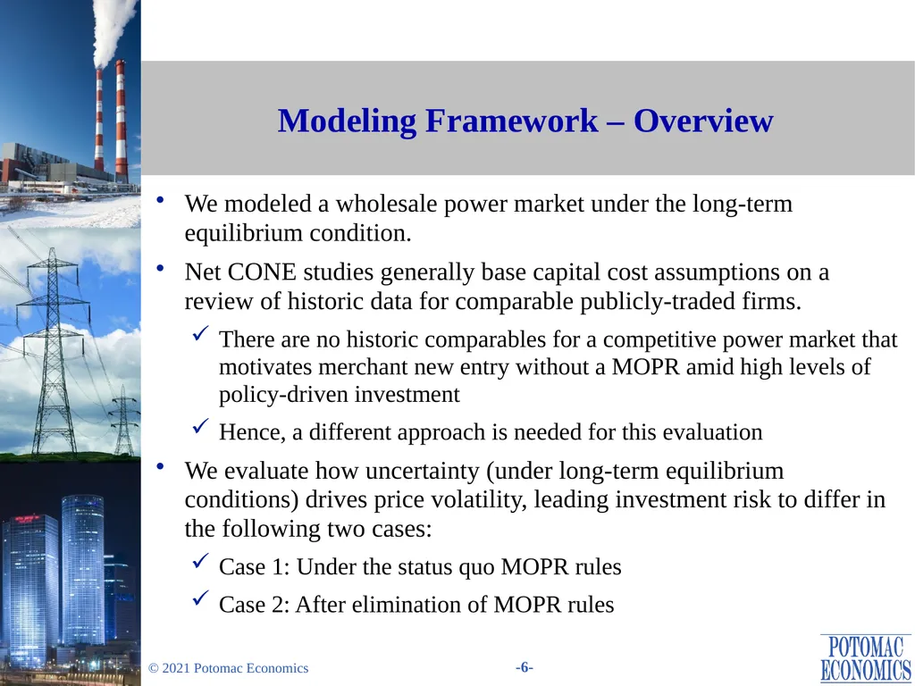
slide6. Modeling Framework – Overview We modeled a wholesale power market under the long-term equilibrium condition.
Net CONE studies generally base capital cost assumptions on a review of historic data for comparable publicly-traded firms.
There are no historic comparables for a competitive power market that motivates merchant new entry without a MOPR amid high levels of policy-driven investment
Hence, a different approach is needed for this evaluation
We evaluate how uncertainty (under long-term equilibrium conditions) drives price volatility, leading investment risk to differ in the following two cases:
Case 1: Under the status quo MOPR rules
Case 2: After elimination of MOPR rules<br>
slide7. Modeling Framework - Cost of Equity The Capital Asset Pricing Model predicts that increasing expected volatility of market revenues will increase the power market risk component of the cost of equity: 
COENoMOPR-P = COEMOPR-P × StDevNoMOPR ÷ StDevMOPR where 
COEMOPR-P is the power market risk component of cost of equity under the MOPR, which we derive from the Net CONE study and recent orders setting regulated ROEs: 
COEMOPR-P = {Merchant cost of equity} minus
{Regulated cost of equity}
StDev is the expected standard deviation of market returns in each case
Using results from a Monte Carlo simulation of the system at long-term equilibrium, we estimated the difference in the standard deviation of market revenues in the MOPR and no MOPR cases.<br>
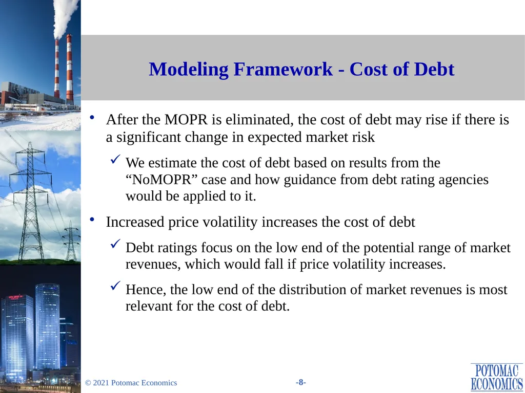
slide8. Modeling Framework - Cost of Debt After the MOPR is eliminated, the cost of debt may rise if there is a significant change in expected market risk
We estimate the cost of debt based on results from the “NoMOPR” case and how guidance from debt rating agencies would be applied to it.
Increased price volatility increases the cost of debt
Debt ratings focus on the low end of the potential range of market revenues, which would fall if price volatility increases.
Hence, the low end of the distribution of market revenues is most relevant for the cost of debt.<br>
slide9. Initial Input Assumptions<br>
slide10. Principles for Determining Model Inputs (1) State policies are driving a rapid increase in penetration of clean resources – New England states have published detailed information about these policies.
There is substantial uncertainty regarding the state policies, including the timing and quantities of new supply over the investment horizon
Some policies lack detail (e.g., whether the policy will focus on solar or wind to achieve certain targets)
Some states have made slower than expected progress toward stated policy goals. (e.g., a project originally contracted with a utility to enter in 2024 might not enter the market until 2028.)
Our assumptions regarding state policies are derived primarily from key documents supporting legislation and/or regulations:
For example: 2050 Decarbonization Roadmap<br>
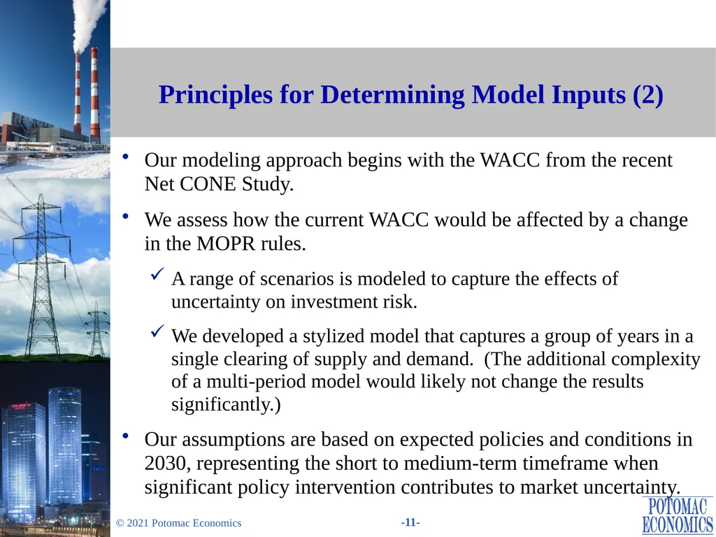
slide11. Principles for Determining Model Inputs (2) Our modeling approach begins with the WACC from the recent Net CONE Study.
We assess how the current WACC would be affected by a change in the MOPR rules.
A range of scenarios is modeled to capture the effects of uncertainty on investment risk.
We developed a stylized model that captures a group of years in a single clearing of supply and demand. (The additional complexity of a multi-period model would likely not change the results significantly.)
Our assumptions are based on expected policies and conditions in 2030, representing the short to medium-term timeframe when significant policy intervention contributes to market uncertainty.<br>
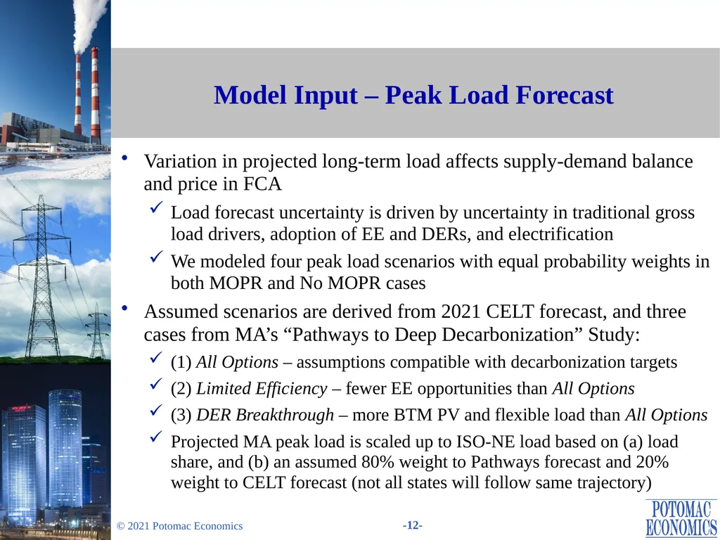
slide12. Model Input – Peak Load Forecast Variation in projected long-term load affects supply-demand balance and price in FCA
Load forecast uncertainty is driven by uncertainty in traditional gross load drivers, adoption of EE and DERs, and electrification
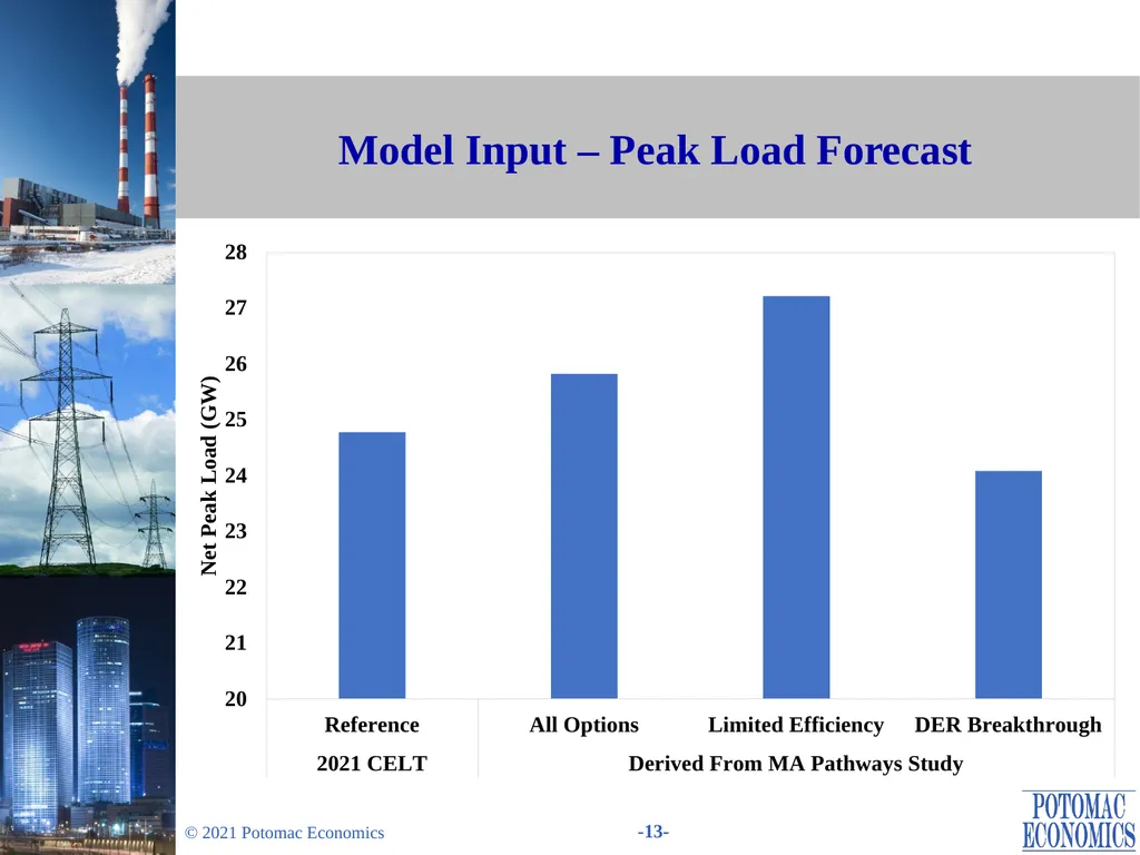
We modeled four peak load scenarios with equal probability weights in both MOPR and No MOPR cases
Assumed scenarios are derived from 2021 CELT forecast, and three cases from MA’s “Pathways to Deep Decarbonization” Study:
(1) All Options – assumptions compatible with decarbonization targets
(2) Limited Efficiency – fewer EE opportunities than All Options
(3) DER Breakthrough – more BTM PV and flexible load than All Options
Projected MA peak load is scaled up to ISO-NE load based on (a) load share, and (b) an assumed 80% weight to Pathways forecast and 20% weight to CELT forecast (not all states will follow same trajectory)<br>
slide13. Model Input – Peak Load Forecast<br>
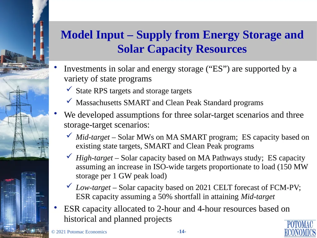
slide14. Model Input – Supply from Energy Storage and Solar Capacity Resources Investments in solar and energy storage (“ES”) are supported by a variety of state programs
State RPS targets and storage targets
Massachusetts SMART and Clean Peak Standard programs
We developed assumptions for three solar-target scenarios and three storage-target scenarios:
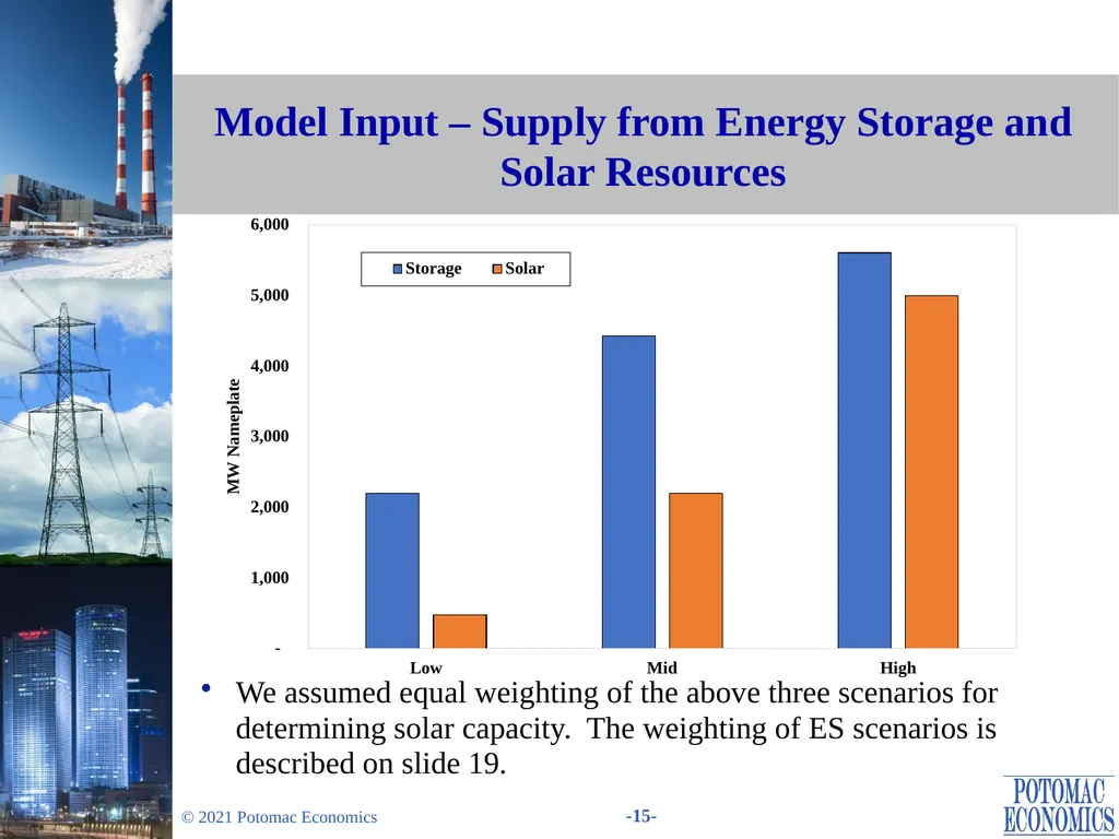
Mid-target – Solar MWs on MA SMART program; ES capacity based on existing state targets, SMART and Clean Peak programs
High-target – Solar capacity based on MA Pathways study; ES capacity assuming an increase in ISO-wide targets proportionate to load (150 MW storage per 1 GW peak load)
Low-target – Solar capacity based on 2021 CELT forecast of FCM-PV; ESR capacity assuming a 50% shortfall in attaining Mid-target
ESR capacity allocated to 2-hour and 4-hour resources based on historical and planned projects<br>
slide15. Model Input – Supply from Energy Storage and Solar Resources We assumed equal weighting of the above three scenarios for determining solar capacity. The weighting of ES scenarios is described on slide 19.<br>
slide16. Model Input – Supply from Energy Storage and Solar Resources We considered synergies between storage and solar in determining the assumed supply from these resources since they can have greater value in combination than individually
The ELCC values were used to quantify the capacity quantities of these resources
ELCC curve for intermittent resources was derived from a 2020 Brattle Group study performed in NY context, but considering comparable quantities of intermittent resources1
Slope of ELCC curves for 2-hour and 4-hour storage resources were derived from a 2019 study by GE2
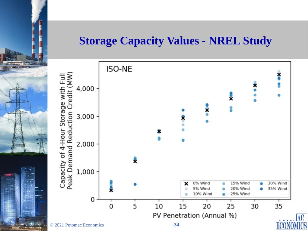
Storage ELCC was adjusted to account for renewable resource penetration based on a 2019 study by NREL (see slide 34)3<br>
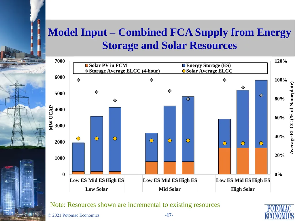
slide17. Model Input – Combined FCA Supply from Energy Storage and Solar Resources Note: Resources shown are incremental to existing resources<br>
slide18. Model Input – Capacity Offers from Solar and Storage Solar resources are price-takers in MOPR and No MOPR cases
Since Class I REC revenues are considered in the offer floor calculation, we assume solar resources will be price-takers
Battery storage are assumed to be subsidized as necessary to meet the target levels on the previous slide, with the possibility of additional merchant storage entry
In No MOPR case, subsidized storage resources are price-takers and additional merchant storage offer at prices described below
In MOPR case, the average offer prices of storage resources are:
For 2-hr units, their ORTP ($2.9/kW-mo in 2030$)
For 4-hr units, a value developed by the IMM’s consultants for its FCA-16 new resource reviews
Offer prices and the probability weights of storage target scenarios are adjusted based on battery costs that are discussed on next slide<br>
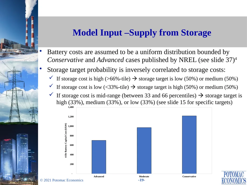
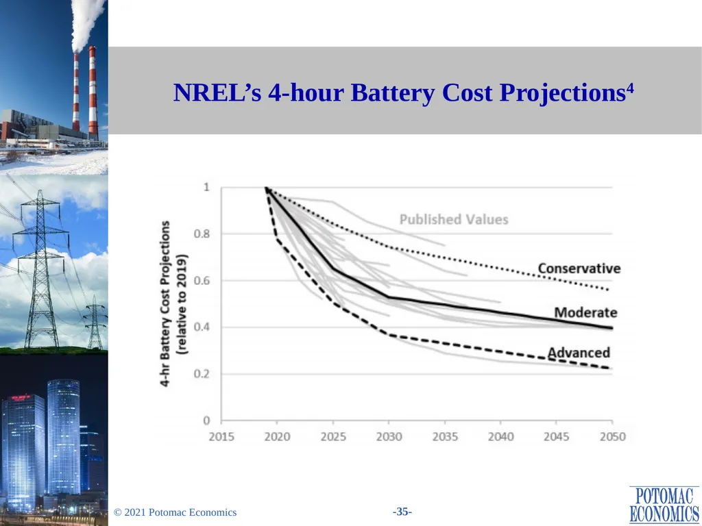
slide19. Model Input –Supply from Storage Battery costs are assumed to be a uniform distribution bounded by Conservative and Advanced cases published by NREL (see slide 37)4
Storage target probability is inversely correlated to storage costs:
If storage cost is high (>66%-tile)  storage target is low (50%) or medium (50%)
If storage cost is low (<33%-tile)  storage target is high (50%) or medium (50%)
If storage cost is mid-range (between 33 and 66 percentiles)  storage target is high (33%), medium (33%), or low (33%) (see slide 15 for specific targets)<br>
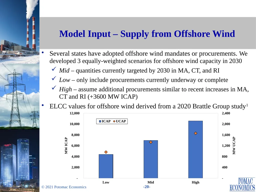
slide20. Model Input – Supply from Offshore Wind Several states have adopted offshore wind mandates or procurements. We developed 3 equally-weighted scenarios for offshore wind capacity in 2030
Mid – quantities currently targeted by 2030 in MA, CT, and RI
Low – only include procurements currently underway or complete
High – assume additional procurements similar to recent increases in MA, CT and RI (+3600 MW ICAP)
ELCC values for offshore wind derived from a 2020 Brattle Group study1<br>
slide21. Model Input – Supply from Existing Resources and New Combustion Turbine Units Existing Resources – Supply from various types of internal resources is based on the actual cleared quantities from FCA-15
Oil/gas-fired steam turbines are assumed to retire or no longer sell capacity due to high GFCs, higher PPR, and poor performance in PFP events
We reviewed Net GFCs for existing CCs and CTs from studies for NEPOOL and NESCOE.5 Given the expected value of PFP events, we assume offers from these resources ranging from $1-$4/kW-mo
New CTs - The ability of fossil-fired resources to be permitted and the availability of sites for building new CTs is unclear
We modeled 4 equally-weighted scenarios with varying quantities (1.5 GW to 6 GW) of feasible new CT builds
We assume that new CTs offer at Net CONE to Net CONE +$1/kW-mo
Supply Adjustment - Since the model is initiated in an equilibrium where: E(Revenues) = Gross CONE, an initial adjustment to the supply is required to satisfy this condition. See slide 25<br>
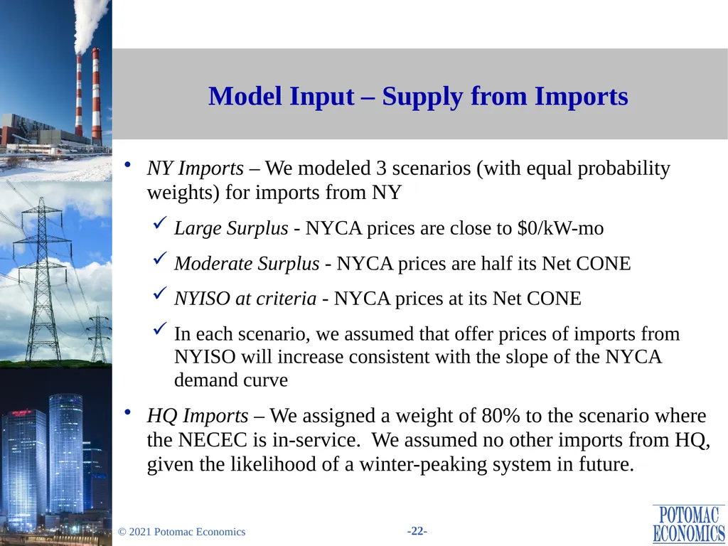
slide22. Model Input – Supply from Imports NY Imports – We modeled 3 scenarios (with equal probability weights) for imports from NY
Large Surplus - NYCA prices are close to $0/kW-mo
Moderate Surplus - NYCA prices are half its Net CONE
NYISO at criteria - NYCA prices at its Net CONE
In each scenario, we assumed that offer prices of imports from NYISO will increase consistent with the slope of the NYCA demand curve
HQ Imports – We assigned a weight of 80% to the scenario where the NECEC is in-service. We assumed no other imports from HQ, given the likelihood of a winter-peaking system in future.<br>
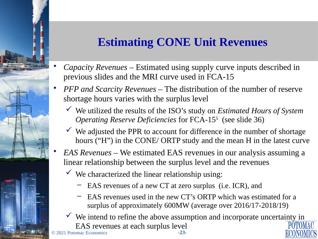
slide23. Estimating CONE Unit Revenues Capacity Revenues – Estimated using supply curve inputs described in previous slides and the MRI curve used in FCA-15
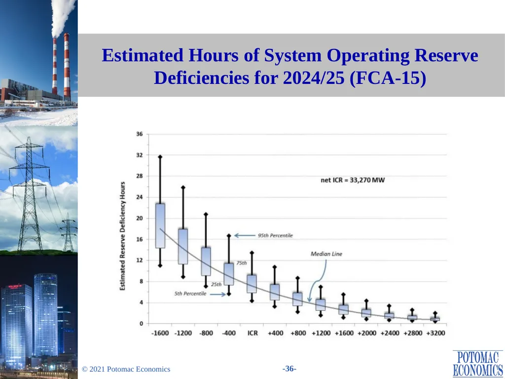
PFP and Scarcity Revenues – The distribution of the number of reserve shortage hours varies with the surplus level
We utilized the results of the ISO’s study on Estimated Hours of System Operating Reserve Deficiencies for FCA-155 (see slide 36)
We adjusted the PPR to account for difference in the number of shortage hours (“H”) in the CONE/ ORTP study and the mean H in the latest curve
EAS Revenues – We estimated EAS revenues in our analysis assuming a linear relationship between the surplus level and the revenues
We characterized the linear relationship using:
EAS revenues of a new CT at zero surplus (i.e. ICR), and
EAS revenues used in the new CT’s ORTP which was estimated for a surplus of approximately 600MW (average over 2016/17-2018/19)
We intend to refine the above assumption and incorporate uncertainty in EAS revenues at each surplus level<br>
slide24. Initial Results<br>
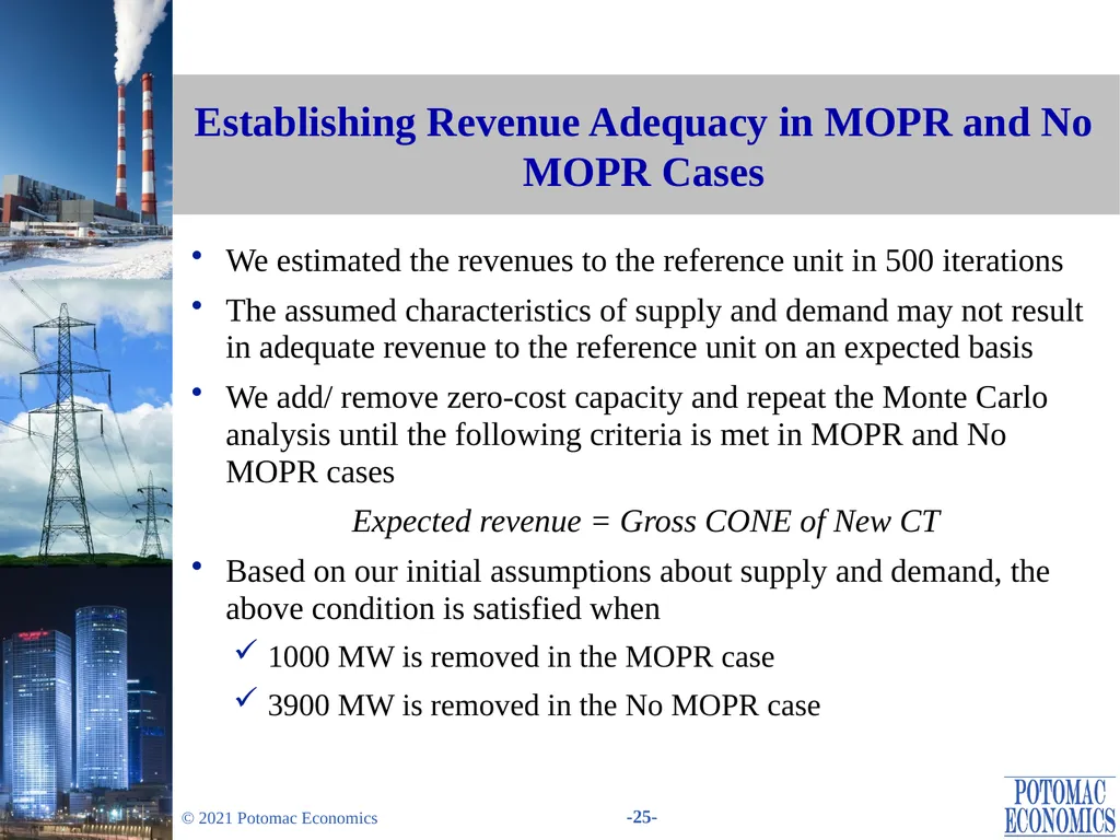
slide25. Establishing Revenue Adequacy in MOPR and No MOPR Cases We estimated the revenues to the reference unit in 500 iterations
The assumed characteristics of supply and demand may not result in adequate revenue to the reference unit on an expected basis
We add/ remove zero-cost capacity and repeat the Monte Carlo analysis until the following criteria is met in MOPR and No MOPR cases
Expected revenue = Gross CONE of New CT
Based on our initial assumptions about supply and demand, the above condition is satisfied when
1000 MW is removed in the MOPR case
3900 MW is removed in the No MOPR case<br>
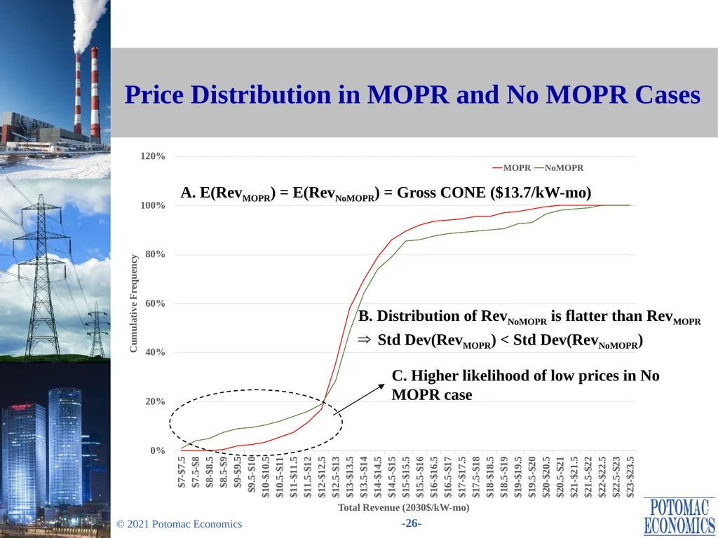
slide26. Price Distribution in MOPR and No MOPR Cases A. E(RevMOPR) = E(RevNoMOPR) = Gross CONE ($13.7/kW-mo) B. Distribution of RevNoMOPR is flatter than RevMOPR
⇒  Std Dev(RevMOPR) < Std Dev(RevNoMOPR) C. Higher likelihood of low prices in No MOPR case<br>
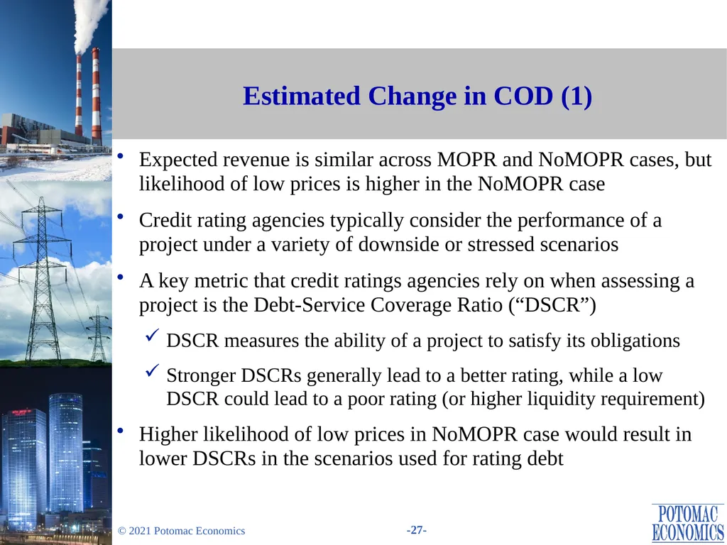
slide27. Estimated Change in COD (1) Expected revenue is similar across MOPR and NoMOPR cases, but likelihood of low prices is higher in the NoMOPR case
Credit rating agencies typically consider the performance of a project under a variety of downside or stressed scenarios
A key metric that credit ratings agencies rely on when assessing a project is the Debt-Service Coverage Ratio (“DSCR”)
DSCR measures the ability of a project to satisfy its obligations
Stronger DSCRs generally lead to a better rating, while a low DSCR could lead to a poor rating (or higher liquidity requirement)
Higher likelihood of low prices in NoMOPR case would result in lower DSCRs in the scenarios used for rating debt<br>
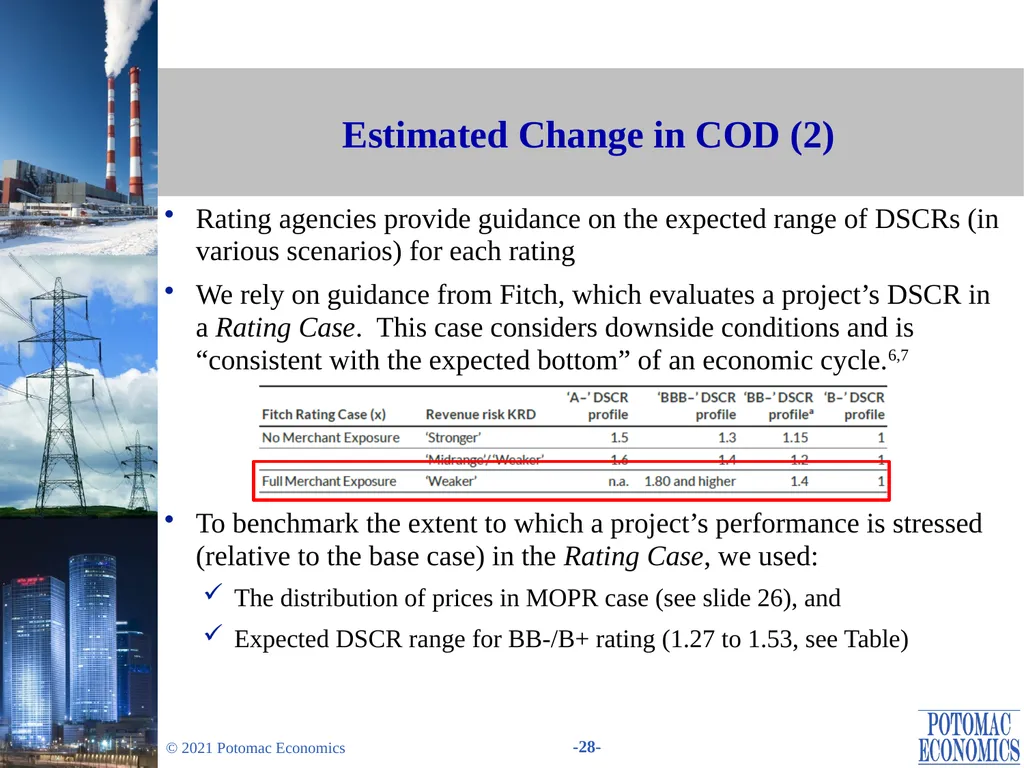
slide28. Estimated Change in COD (2) Rating agencies provide guidance on the expected range of DSCRs (in various scenarios) for each rating
We rely on guidance from Fitch, which evaluates a project’s DSCR in a Rating Case. This case considers downside conditions and is “consistent with the expected bottom” of an economic cycle.6,7

To benchmark the extent to which a project’s performance is stressed (relative to the base case) in the Rating Case, we used:
The distribution of prices in MOPR case (see slide 26), and
Expected DSCR range for BB-/B+ rating (1.27 to 1.53, see Table)<br>
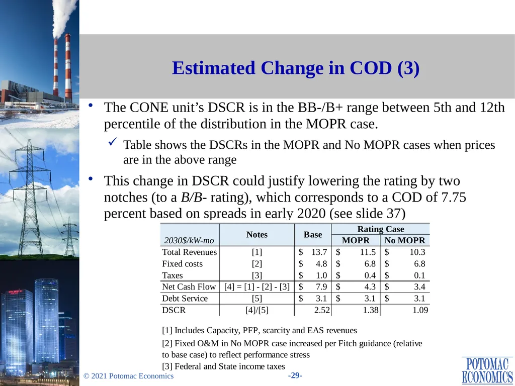
slide29. Estimated Change in COD (3) The CONE unit’s DSCR is in the BB-/B+ range between 5th and 12th percentile of the distribution in the MOPR case.
Table shows the DSCRs in the MOPR and No MOPR cases when prices are in the above range
This change in DSCR could justify lowering the rating by two notches (to a B/B- rating), which corresponds to a COD of 7.75 percent based on spreads in early 2020 (see slide 37)<br>
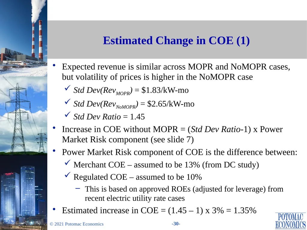
slide30. Estimated Change in COE (1) Expected revenue is similar across MOPR and NoMOPR cases, but volatility of prices is higher in the NoMOPR case
Std Dev(RevMOPR) = $1.83/kW-mo
Std Dev(RevNoMOPR) = $2.65/kW-mo
Std Dev Ratio = 1.45
Increase in COE without MOPR = (Std Dev Ratio-1) x Power Market Risk component (see slide 7)
Power Market Risk component of COE is the difference between:
Merchant COE – assumed to be 13% (from DC study)
Regulated COE – assumed to be 10%
This is based on approved ROEs (adjusted for leverage) from recent electric utility rate cases
Estimated increase in COE = (1.45 – 1) x 3% = 1.35%<br>
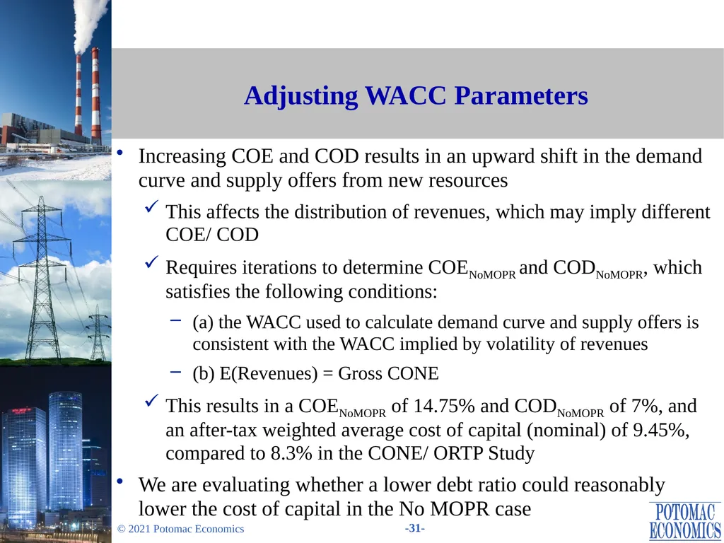
slide31. Adjusting WACC Parameters Increasing COE and COD results in an upward shift in the demand curve and supply offers from new resources
This affects the distribution of revenues, which may imply different COE/ COD
Requires iterations to determine COENoMOPR and CODNoMOPR, which satisfies the following conditions:
(a) the WACC used to calculate demand curve and supply offers is consistent with the WACC implied by volatility of revenues
(b) E(Revenues) = Gross CONE
This results in a COENoMOPR of 14.75% and CODNoMOPR of 7%, and an after-tax weighted average cost of capital (nominal) of 9.45%, compared to 8.3% in the CONE/ ORTP Study
We are evaluating whether a lower debt ratio could reasonably lower the cost of capital in the No MOPR case<br>
slide32. Questions?<br>
slide33. Appendix<br>
slide34. Storage Capacity Values - NREL Study<br>
slide35. NREL’s 4-hour Battery Cost Projections4<br>
slide36. Estimated Hours of System Operating Reserve Deficiencies for 2024/25 (FCA-15)<br>
slide37. Bond Yields The following table shows the assumed corporate bond yields for B and BB-rated bonds

The yields shown are derived from:
Corporate BB and B index yields for the January-June 2020, published by FRED (Federal Reserve St. Louis)
Spread for each rating from January 2021 published by Professor Damodaran of Stern School of Business8<br>
slide38. References (1) [1] The Brattle Group (2020), “Quantitative Analysis of Resource Adequacy Structures”
[2] GE Energy Consulting (2019), “Valuing Capacity for Resources with Energy Limitations”
[3] Denholm, Nunemaker, Gagnon and Cole (2019), “The Potential for Battery Energy Storage to Provide Peaking Capacity in the United States.”
[4] NREL (2021), Annual Technology Baseline
[5] Operating Reserve Deficiency Information – Capacity Commitment Period 2024-2025
[6] FitchRatings (2021), Thermal Power Project Rating Criteria
[7] FitchRatings (2020), Infrastructure and Project Finance Rating Criteria
[8] Damodaran (2021), Ratings, Interest Coverage Ratios and Default Spread<br>