
Graphs Chapter 10 With Question/Answer Animations
MT
Published · 89 slides · 0 views
1 / 1

Description
Graphs Chapter 10 With QuestionAnswer Animations McGraw Hill LLC. All rights reserved. No reproduction or distribution without the prior written consent of McGraw Hill LLC. Chapter Summary Graphs and Graph Models. Graph Terminology and
Related Topics
Share
Embed code
Download this presentation From Below
"Graphs Chapter 10 With Question/Answer Animations" is the property of its rightful owner. Permission is granted to download and print the materials on this website for personal, non-commercial use only, and to display it on your personal computer provided you do not modify the materials and that you retain all copyright notices contained in the materials. By downloading content from our website, you accept the terms of this agreement.
Presentation Transcript
01
Graphs Chapter 10 With Question/Answer Animations © McGraw Hill LLC. All rights reserved. No reproduction or distribution without the prior written consent of McGraw Hill LLC.<br>
02
Chapter Summary Graphs and Graph Models.
Graph Terminology and Special Types of Graphs.
Representing Graphs and Graph Isomorphism Connectivity.
Euler and Hamiltonian Graphs.
Shortest-Path Problems (not currently included in overheads).
Planar Graphs (not currently included in overheads).
Graph Coloring (not currently included in overheads). 2<br>
Graph Terminology and Special Types of Graphs.
Representing Graphs and Graph Isomorphism Connectivity.
Euler and Hamiltonian Graphs.
Shortest-Path Problems (not currently included in overheads).
Planar Graphs (not currently included in overheads).
Graph Coloring (not currently included in overheads). 2<br>
03
Graphs and Graph Models Section 10.1 3<br>
04
Section Summary 1 Introduction to Graphs.
Graph Taxonomy.
Graph Models. 4<br>
Graph Taxonomy.
Graph Models. 4<br>
05
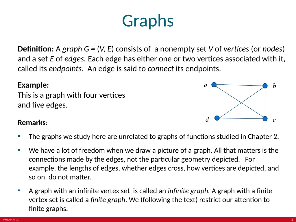
Graphs Definition: A graph G = (V, E) consists of a nonempty set V of vertices (or nodes) and a set E of edges. Each edge has either one or two vertices associated with it, called its endpoints. An edge is said to connect its endpoints. Example:
This is a graph with four vertices and five edges. Remarks:
The graphs we study here are unrelated to graphs of functions studied in Chapter 2.
We have a lot of freedom when we draw a picture of a graph. All that matters is the connections made by the edges, not the particular geometry depicted. For example, the lengths of edges, whether edges cross, how vertices are depicted, and so on, do not matter.
A graph with an infinite vertex set is called an infinite graph. A graph with a finite vertex set is called a finite graph. We (following the text) restrict our attention to finite graphs. 5<br>
The graphs we study here are unrelated to graphs of functions studied in Chapter 2.
We have a lot of freedom when we draw a picture of a graph. All that matters is the connections made by the edges, not the particular geometry depicted. For example, the lengths of edges, whether edges cross, how vertices are depicted, and so on, do not matter.
A graph with an infinite vertex set is called an infinite graph. A graph with a finite vertex set is called a finite graph. We (following the text) restrict our attention to finite graphs. 5<br>
06
Some Terminology 1 In a simple graph each edge connects two different vertices and no two edges connect the same pair of vertices.
Multigraphs may have multiple edges connecting the same two vertices. When m different edges connect the vertices u and v, we say that {u,v} is an edge of multiplicity m.
An edge that connects a vertex to itself is called a loop.
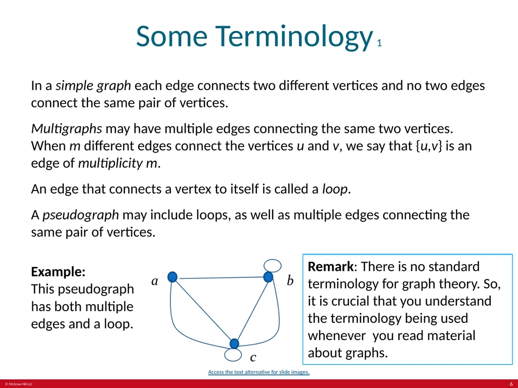
A pseudograph may include loops, as well as multiple edges connecting the same pair of vertices. Example: This pseudograph has both multiple edges and a loop. Remark: There is no standard terminology for graph theory. So, it is crucial that you understand the terminology being used whenever you read material about graphs. Access the text alternative for slide images. 6<br>
Multigraphs may have multiple edges connecting the same two vertices. When m different edges connect the vertices u and v, we say that {u,v} is an edge of multiplicity m.
An edge that connects a vertex to itself is called a loop.
A pseudograph may include loops, as well as multiple edges connecting the same pair of vertices. Example: This pseudograph has both multiple edges and a loop. Remark: There is no standard terminology for graph theory. So, it is crucial that you understand the terminology being used whenever you read material about graphs. Access the text alternative for slide images. 6<br>
07
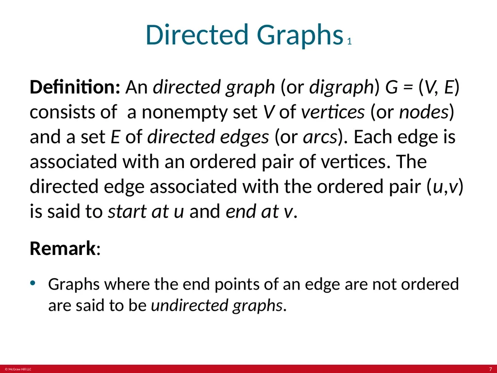
Directed Graphs 1 Definition: An directed graph (or digraph) G = (V, E) consists of a nonempty set V of vertices (or nodes) and a set E of directed edges (or arcs). Each edge is associated with an ordered pair of vertices. The directed edge associated with the ordered pair (u,v) is said to start at u and end at v.
Remark:
Graphs where the end points of an edge are not ordered are said to be undirected graphs. 7<br>
Remark:
Graphs where the end points of an edge are not ordered are said to be undirected graphs. 7<br>
08
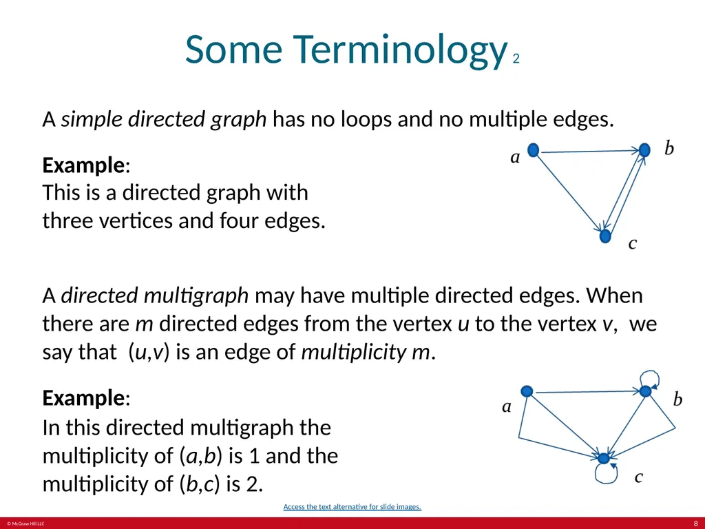
Some Terminology 2 A simple directed graph has no loops and no multiple edges.
Example: This is a directed graph with three vertices and four edges. A directed multigraph may have multiple directed edges. When there are m directed edges from the vertex u to the vertex v, we say that (u,v) is an edge of multiplicity m.
Example: In this directed multigraph the multiplicity of (a,b) is 1 and the multiplicity of (b,c) is 2. Access the text alternative for slide images. 8<br>
Example: This is a directed graph with three vertices and four edges. A directed multigraph may have multiple directed edges. When there are m directed edges from the vertex u to the vertex v, we say that (u,v) is an edge of multiplicity m.
Example: In this directed multigraph the multiplicity of (a,b) is 1 and the multiplicity of (b,c) is 2. Access the text alternative for slide images. 8<br>
09
Graph Models:
Computer Networks 1 When we build a graph model, we use the appropriate type of graph to capture the important features of the application.
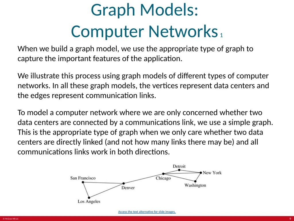
We illustrate this process using graph models of different types of computer networks. In all these graph models, the vertices represent data centers and the edges represent communication links.
To model a computer network where we are only concerned whether two data centers are connected by a communications link, we use a simple graph. This is the appropriate type of graph when we only care whether two data centers are directly linked (and not how many links there may be) and all communications links work in both directions. Access the text alternative for slide images. 9<br>
We illustrate this process using graph models of different types of computer networks. In all these graph models, the vertices represent data centers and the edges represent communication links.
To model a computer network where we are only concerned whether two data centers are connected by a communications link, we use a simple graph. This is the appropriate type of graph when we only care whether two data centers are directly linked (and not how many links there may be) and all communications links work in both directions. Access the text alternative for slide images. 9<br>
10
Graph Models:
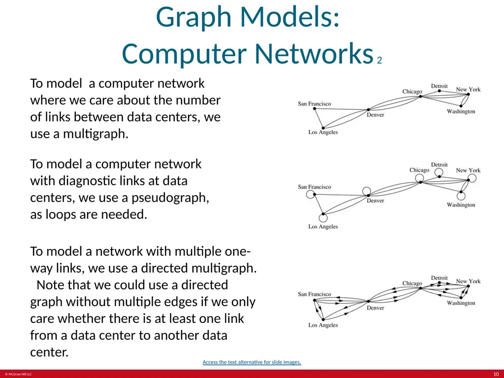
Computer Networks 2 To model a computer network where we care about the number of links between data centers, we use a multigraph. To model a computer network with diagnostic links at data centers, we use a pseudograph, as loops are needed. To model a network with multiple one-way links, we use a directed multigraph. Note that we could use a directed graph without multiple edges if we only care whether there is at least one link from a data center to another data center. Access the text alternative for slide images. 10<br>
11
Graph Terminology: Summary To understand the structure of a graph and to build a graph model, we ask these questions:
Are the edges of the graph undirected or directed (or both)?
If the edges are undirected, are multiple edges present that connect the same pair of vertices? If the edges are directed, are multiple directed edges present?
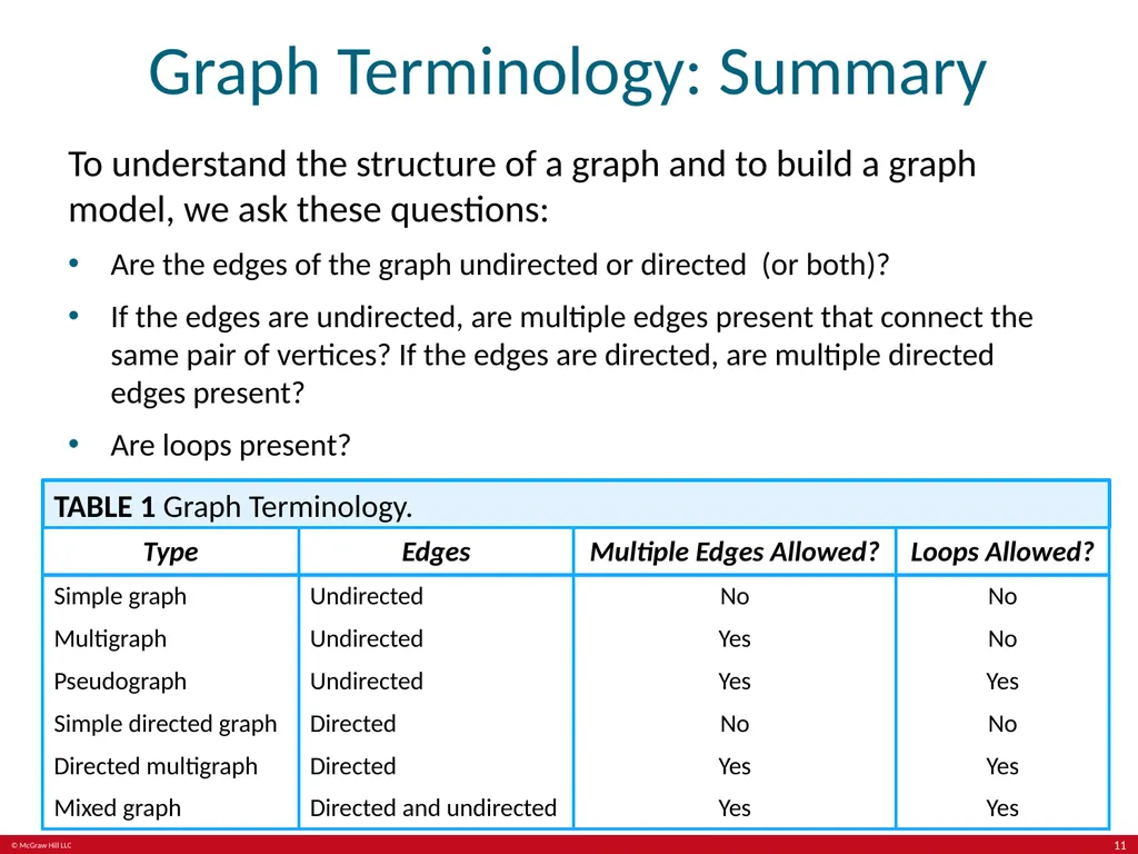
Are loops present? TABLE 1 Graph Terminology. 11<br>
Are the edges of the graph undirected or directed (or both)?
If the edges are undirected, are multiple edges present that connect the same pair of vertices? If the edges are directed, are multiple directed edges present?
Are loops present? TABLE 1 Graph Terminology. 11<br>
12
Other Applications of Graphs We will illustrate how graph theory can be used in models of:
Social networks.
Communications networks.
Information networks.
Software design.
Transportation networks.
Biological networks.
It’s a challenge to find a subject to which graph theory has not yet been applied. Can you find an area without applications of graph theory? 12<br>
Social networks.
Communications networks.
Information networks.
Software design.
Transportation networks.
Biological networks.
It’s a challenge to find a subject to which graph theory has not yet been applied. Can you find an area without applications of graph theory? 12<br>
13
Graph Models: Social Networks 1 Graphs can be used to model social structures based on different kinds of relationships between people or groups.
In a social network, vertices represent individuals or organizations and edges represent relationships between them.
Useful graph models of social networks include:
friendship graphs - undirected graphs where two people are connected if they are friends (in the real world, on Facebook, or in a particular virtual world, and so on.)
collaboration graphs - undirected graphs where two people are connected if they collaborate in a specific way.
influence graphs - directed graphs where there is an edge from one person to another if the first person can influence the second person. 13<br>
In a social network, vertices represent individuals or organizations and edges represent relationships between them.
Useful graph models of social networks include:
friendship graphs - undirected graphs where two people are connected if they are friends (in the real world, on Facebook, or in a particular virtual world, and so on.)
collaboration graphs - undirected graphs where two people are connected if they collaborate in a specific way.
influence graphs - directed graphs where there is an edge from one person to another if the first person can influence the second person. 13<br>
14
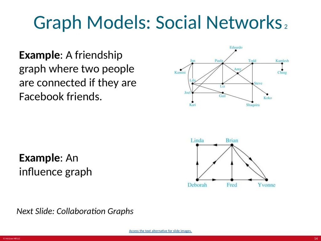
Graph Models: Social Networks 2 Example: A friendship graph where two people are connected if they are Facebook friends. Example: An influence graph Next Slide: Collaboration Graphs Access the text alternative for slide images. 14<br>
15
Examples of Collaboration Graphs The Hollywood graph models the collaboration of actors in films.
We represent actors by vertices and we connect two vertices if the actors they represent have appeared in the same movie.
We will study the Hollywood Graph in Section 10.4 when we discuss Kevin Bacon numbers.
An academic collaboration graph models the collaboration of researchers who have jointly written a paper in a particular subject.
We represent researchers in a particular academic discipline using vertices.
We connect the vertices representing two researchers in this discipline if they are coauthors of a paper.
We will study the academic collaboration graph for mathematicians when we discuss Erdős numbers in Section 10.4. 15<br>
We represent actors by vertices and we connect two vertices if the actors they represent have appeared in the same movie.
We will study the Hollywood Graph in Section 10.4 when we discuss Kevin Bacon numbers.
An academic collaboration graph models the collaboration of researchers who have jointly written a paper in a particular subject.
We represent researchers in a particular academic discipline using vertices.
We connect the vertices representing two researchers in this discipline if they are coauthors of a paper.
We will study the academic collaboration graph for mathematicians when we discuss Erdős numbers in Section 10.4. 15<br>
16
Applications to Information Networks Graphs can be used to model different types of networks that link different types of information.
In a web graph, web pages are represented by vertices and links are represented by directed edges.
A web graph models the web at a particular time.
We will explain how the web graph is used by search engines in Section 11.4.
In a citation network:
Research papers in a particular discipline are represented by vertices.
When a paper cites a second paper as a reference, there is an edge from the vertex representing this paper to the vertex representing the second paper. 16<br>
In a web graph, web pages are represented by vertices and links are represented by directed edges.
A web graph models the web at a particular time.
We will explain how the web graph is used by search engines in Section 11.4.
In a citation network:
Research papers in a particular discipline are represented by vertices.
When a paper cites a second paper as a reference, there is an edge from the vertex representing this paper to the vertex representing the second paper. 16<br>
17
Transportation Graphs Graph models are extensively used in the study of transportation networks.
Airline networks can be modeled using directed multigraphs where
airports are represented by vertices.
each flight is represented by a directed edge from the vertex representing the departure airport to the vertex representing the destination airport.
Road networks can be modeled using graphs where
vertices represent intersections and edges represent roads.
undirected edges represent two-way roads and directed edges represent one-way roads. 17<br>
Airline networks can be modeled using directed multigraphs where
airports are represented by vertices.
each flight is represented by a directed edge from the vertex representing the departure airport to the vertex representing the destination airport.
Road networks can be modeled using graphs where
vertices represent intersections and edges represent roads.
undirected edges represent two-way roads and directed edges represent one-way roads. 17<br>
18
Software Design Applications 1 Graph models are extensively used in software design. We will introduce two such models here; one representing the dependency between the modules of a software application and the other representing restrictions in the execution of statements in computer programs.
When a top-down approach is used to design software, the system is divided into modules, each performing a specific task.
We use a module dependency graph to represent the dependency between these modules. These dependencies need to be understood before coding can be done.
In a module dependency graph vertices represent software modules and there is an edge from one module to another if the second module depends on the first. Example: The dependencies between the seven modules in the design of a web browser are represented by this module dependency graph. Access the text alternative for slide images. 18<br>
When a top-down approach is used to design software, the system is divided into modules, each performing a specific task.
We use a module dependency graph to represent the dependency between these modules. These dependencies need to be understood before coding can be done.
In a module dependency graph vertices represent software modules and there is an edge from one module to another if the second module depends on the first. Example: The dependencies between the seven modules in the design of a web browser are represented by this module dependency graph. Access the text alternative for slide images. 18<br>
19
Software Design Applications 2 We can use a directed graph called a precedence graph to represent which statements must have already been executed before we execute each statement.
Vertices represent statements in a computer program.
There is a directed edge from a vertex to a second vertex if the second vertex cannot be executed before the first. Example: This precedence graph shows which statements must already have been executed before we can execute each of the six statements in the program. Access the text alternative for slide images. 19<br>
Vertices represent statements in a computer program.
There is a directed edge from a vertex to a second vertex if the second vertex cannot be executed before the first. Example: This precedence graph shows which statements must already have been executed before we can execute each of the six statements in the program. Access the text alternative for slide images. 19<br>
20
Biological Applications 1 Graph models are used extensively in many areas of the biological science. We will describe two such models, one to ecology and the other to molecular biology.
Niche overlap graphs model competition between species in an ecosystem
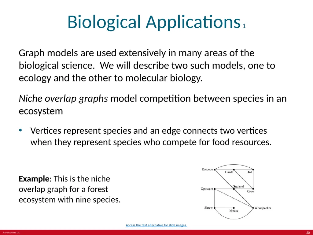
Vertices represent species and an edge connects two vertices when they represent species who compete for food resources. Example: This is the niche overlap graph for a forest ecosystem with nine species. Access the text alternative for slide images. 20<br>
Niche overlap graphs model competition between species in an ecosystem
Vertices represent species and an edge connects two vertices when they represent species who compete for food resources. Example: This is the niche overlap graph for a forest ecosystem with nine species. Access the text alternative for slide images. 20<br>
21
Biological Applications 2 We can model the interaction of proteins in a cell using a protein interaction network.
In a protein interaction graph, vertices represent proteins and vertices are connected by an edge if the proteins they represent interact.
Protein interaction graphs can be huge and can contain more than 100,000 vertices, each representing a different protein, and more than 1,000,000 edges, each representing an interaction between proteins.
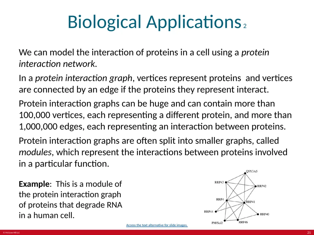
Protein interaction graphs are often split into smaller graphs, called modules, which represent the interactions between proteins involved in a particular function. Example: This is a module of the protein interaction graph of proteins that degrade RNA in a human cell. Access the text alternative for slide images. 21<br>
In a protein interaction graph, vertices represent proteins and vertices are connected by an edge if the proteins they represent interact.
Protein interaction graphs can be huge and can contain more than 100,000 vertices, each representing a different protein, and more than 1,000,000 edges, each representing an interaction between proteins.
Protein interaction graphs are often split into smaller graphs, called modules, which represent the interactions between proteins involved in a particular function. Example: This is a module of the protein interaction graph of proteins that degrade RNA in a human cell. Access the text alternative for slide images. 21<br>
22
Graph Terminology and Special Types of Graphs Section 10.2 22<br>
23
Section Summary 2 Basic Terminology.
Some Special Types of Graphs.
Bipartite Graphs.
Bipartite Graphs and Matchings (not currently included in overheads).
Some Applications of Special Types of Graphs (not currently included in overheads).
New Graphs from Old. 23<br>
Some Special Types of Graphs.
Bipartite Graphs.
Bipartite Graphs and Matchings (not currently included in overheads).
Some Applications of Special Types of Graphs (not currently included in overheads).
New Graphs from Old. 23<br>
24
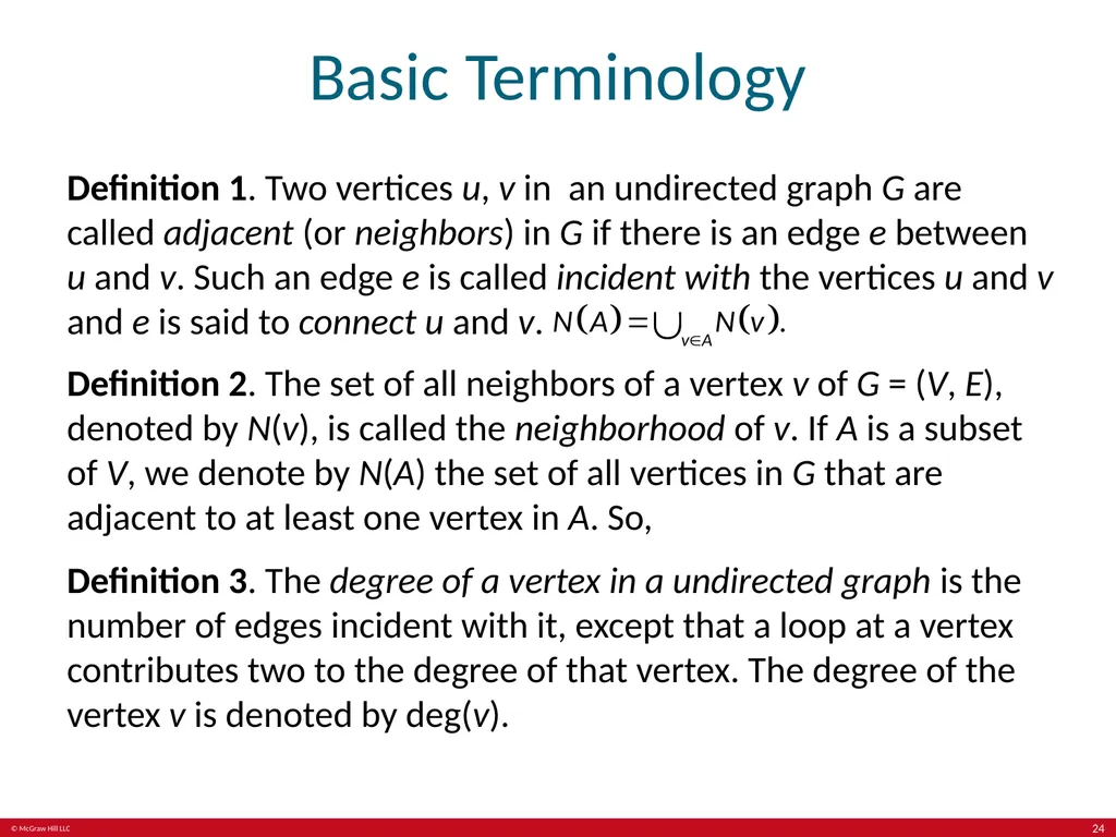
Basic Terminology Definition 1. Two vertices u, v in an undirected graph G are called adjacent (or neighbors) in G if there is an edge e between u and v. Such an edge e is called incident with the vertices u and v and e is said to connect u and v. Definition 2. The set of all neighbors of a vertex v of G = (V, E), denoted by N(v), is called the neighborhood of v. If A is a subset of V, we denote by N(A) the set of all vertices in G that are adjacent to at least one vertex in A. So,
Definition 3. The degree of a vertex in a undirected graph is the number of edges incident with it, except that a loop at a vertex contributes two to the degree of that vertex. The degree of the vertex v is denoted by deg(v). 24<br>
Definition 3. The degree of a vertex in a undirected graph is the number of edges incident with it, except that a loop at a vertex contributes two to the degree of that vertex. The degree of the vertex v is denoted by deg(v). 24<br>
25
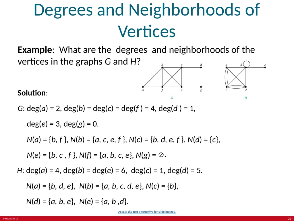
Degrees and Neighborhoods of Vertices Example: What are the degrees and neighborhoods of the vertices in the graphs G and H? Solution:
G: deg(a) = 2, deg(b) = deg(c) = deg(f ) = 4, deg(d ) = 1,
deg(e) = 3, deg(g) = 0.
N(a) = {b, f }, N(b) = {a, c, e, f }, N(c) = {b, d, e, f }, N(d) = {c},
N(e) = {b, c , f }, N(f) = {a, b, c, e}, N(g) = H: deg(a) = 4, deg(b) = deg(e) = 6, deg(c) = 1, deg(d) = 5.
N(a) = {b, d, e}, N(b) = {a, b, c, d, e}, N(c) = {b},
N(d) = {a, b, e}, N(e) = {a, b ,d}. Access the text alternative for slide images. 25<br>
G: deg(a) = 2, deg(b) = deg(c) = deg(f ) = 4, deg(d ) = 1,
deg(e) = 3, deg(g) = 0.
N(a) = {b, f }, N(b) = {a, c, e, f }, N(c) = {b, d, e, f }, N(d) = {c},
N(e) = {b, c , f }, N(f) = {a, b, c, e}, N(g) = H: deg(a) = 4, deg(b) = deg(e) = 6, deg(c) = 1, deg(d) = 5.
N(a) = {b, d, e}, N(b) = {a, b, c, d, e}, N(c) = {b},
N(d) = {a, b, e}, N(e) = {a, b ,d}. Access the text alternative for slide images. 25<br>
26
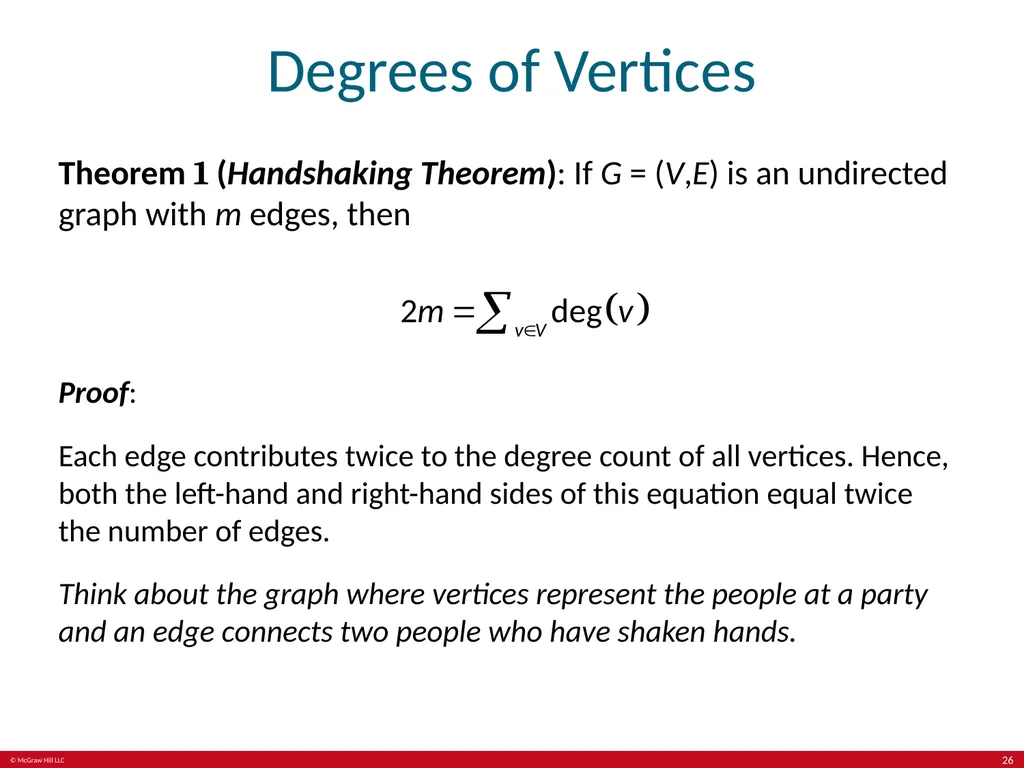
Degrees of Vertices Theorem 1 (Handshaking Theorem): If G = (V,E) is an undirected graph with m edges, then Proof:
Each edge contributes twice to the degree count of all vertices. Hence, both the left-hand and right-hand sides of this equation equal twice the number of edges.
Think about the graph where vertices represent the people at a party and an edge connects two people who have shaken hands. 26<br>
Each edge contributes twice to the degree count of all vertices. Hence, both the left-hand and right-hand sides of this equation equal twice the number of edges.
Think about the graph where vertices represent the people at a party and an edge connects two people who have shaken hands. 26<br>
27
Handshaking Theorem We now give two examples illustrating the usefulness of the handshaking theorem.
Example: How many edges are there in a graph with 10 vertices of degree six?
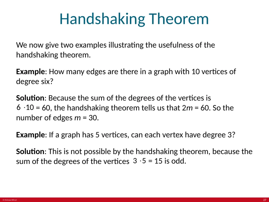
Solution: Because the sum of the degrees of the vertices is = 60, the handshaking theorem tells us that 2m = 60. So the number of edges m = 30. Example: If a graph has 5 vertices, can each vertex have degree 3?
Solution: This is not possible by the handshaking theorem, because the sum of the degrees of the vertices = 15 is odd. 27<br>
Example: How many edges are there in a graph with 10 vertices of degree six?
Solution: Because the sum of the degrees of the vertices is = 60, the handshaking theorem tells us that 2m = 60. So the number of edges m = 30. Example: If a graph has 5 vertices, can each vertex have degree 3?
Solution: This is not possible by the handshaking theorem, because the sum of the degrees of the vertices = 15 is odd. 27<br>
28
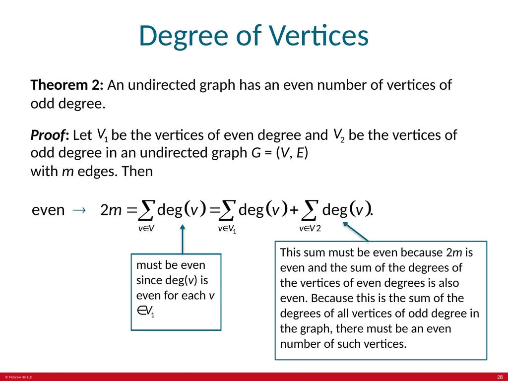
Degree of Vertices Theorem 2: An undirected graph has an even number of vertices of odd degree.
Proof: Let be the vertices of even degree and be the vertices of odd degree in an undirected graph G = (V, E) with m edges. Then must be even since deg(v) is even for each v ∈ This sum must be even because 2m is even and the sum of the degrees of the vertices of even degrees is also even. Because this is the sum of the degrees of all vertices of odd degree in the graph, there must be an even number of such vertices. 28<br>
Proof: Let be the vertices of even degree and be the vertices of odd degree in an undirected graph G = (V, E) with m edges. Then must be even since deg(v) is even for each v ∈ This sum must be even because 2m is even and the sum of the degrees of the vertices of even degrees is also even. Because this is the sum of the degrees of all vertices of odd degree in the graph, there must be an even number of such vertices. 28<br>
29
Directed Graphs 2 Recall the definition of a directed graph.
Definition: An directed graph G = (V, E) consists of V, a nonempty set of vertices (or nodes), and E, a set of directed edges or arcs. Each edge is an ordered pair of vertices. The directed edge (u,v) is said to start at u and end at v.
Definition: Let (u,v) be an edge in G. Then u is the initial vertex of this edge and is adjacent to v and v is the terminal (or end) vertex of this edge and is adjacent from u. The initial and terminal vertices of a loop are the same. 29<br>
Definition: An directed graph G = (V, E) consists of V, a nonempty set of vertices (or nodes), and E, a set of directed edges or arcs. Each edge is an ordered pair of vertices. The directed edge (u,v) is said to start at u and end at v.
Definition: Let (u,v) be an edge in G. Then u is the initial vertex of this edge and is adjacent to v and v is the terminal (or end) vertex of this edge and is adjacent from u. The initial and terminal vertices of a loop are the same. 29<br>
30
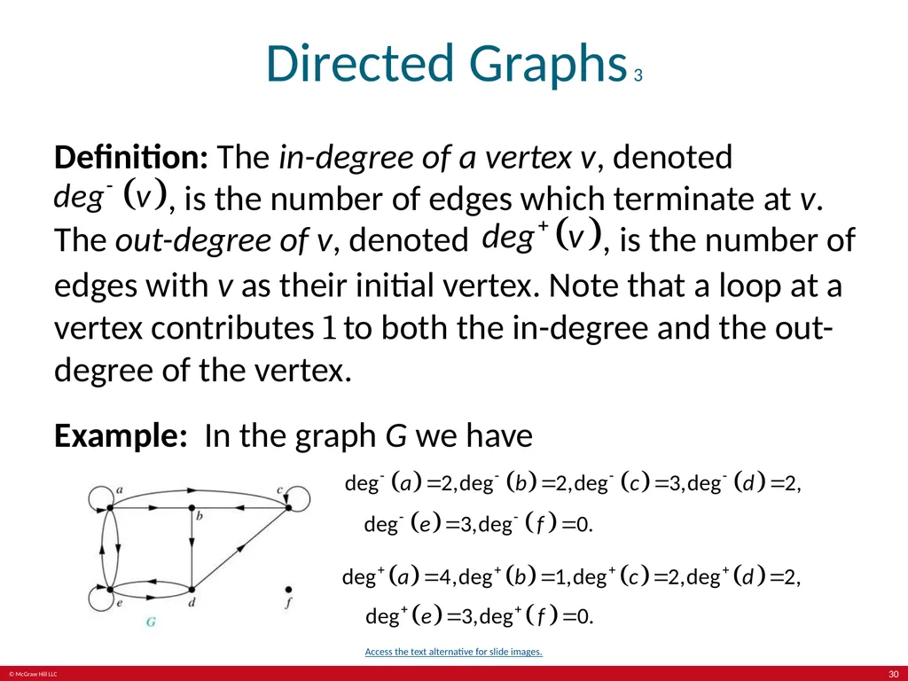
Directed Graphs 3 Definition: The in-degree of a vertex v, denoted , is the number of edges which terminate at v. The out-degree of v, denoted , is the number of edges with v as their initial vertex. Note that a loop at a vertex contributes 1 to both the in-degree and the out-degree of the vertex.
Example: In the graph G we have Access the text alternative for slide images. 30<br>
Example: In the graph G we have Access the text alternative for slide images. 30<br>
31
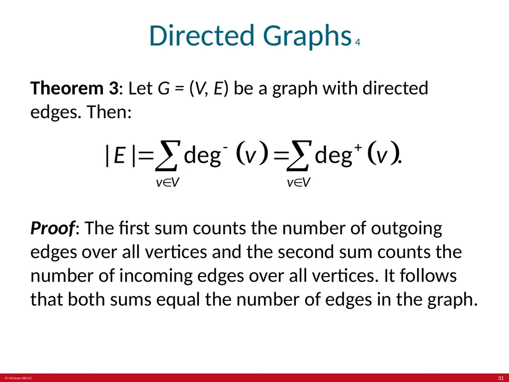
Directed Graphs 4 Theorem 3: Let G = (V, E) be a graph with directed edges. Then: Proof: The first sum counts the number of outgoing edges over all vertices and the second sum counts the number of incoming edges over all vertices. It follows that both sums equal the number of edges in the graph. 31<br>
32
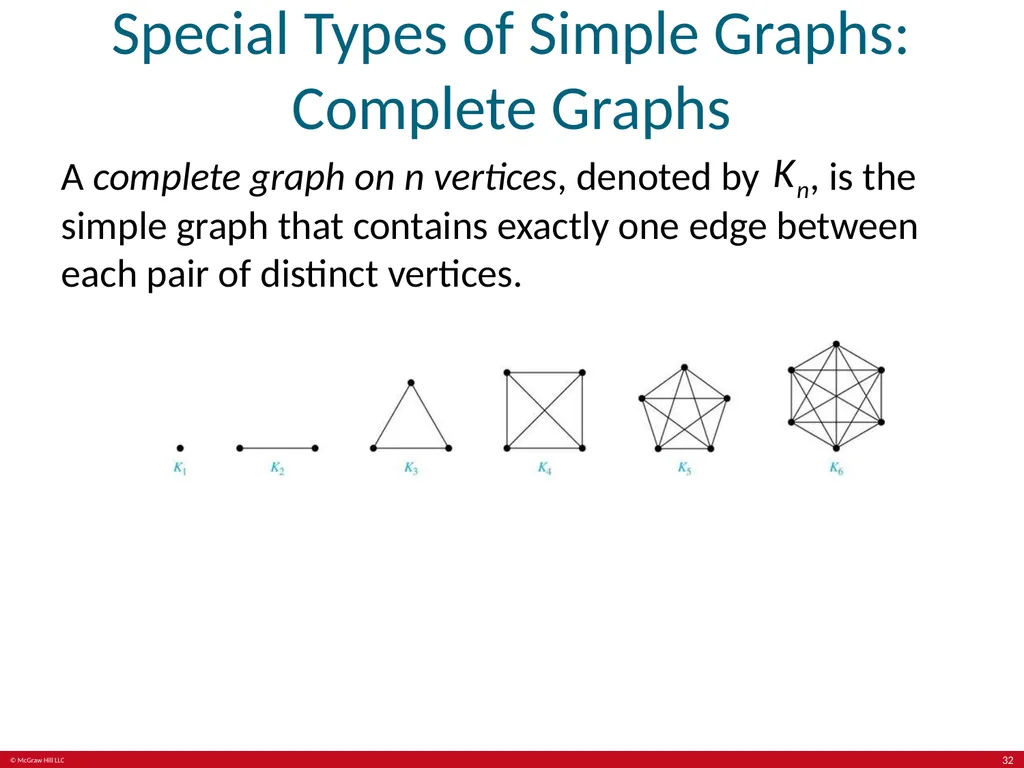
Special Types of Simple Graphs: Complete Graphs A complete graph on n vertices, denoted by , is the simple graph that contains exactly one edge between each pair of distinct vertices. 32<br>
33
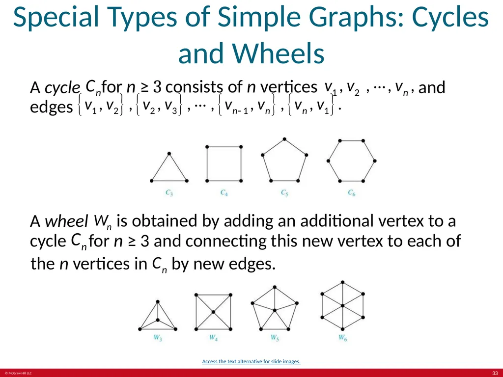
Special Types of Simple Graphs: Cycles and Wheels A cycle for n ≥ 3 consists of n vertices and edges A wheel is obtained by adding an additional vertex to a cycle for n ≥ 3 and connecting this new vertex to each of the n vertices in by new edges. Access the text alternative for slide images. 33<br>
34
Special Types of Simple Graphs:
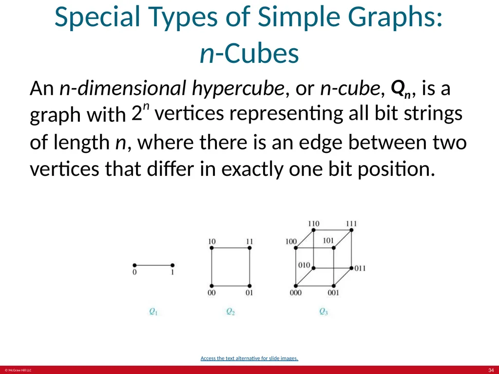
n-Cubes An n-dimensional hypercube, or n-cube, , is a graph with vertices representing all bit strings of length n, where there is an edge between two vertices that differ in exactly one bit position. Access the text alternative for slide images. 34<br>
35
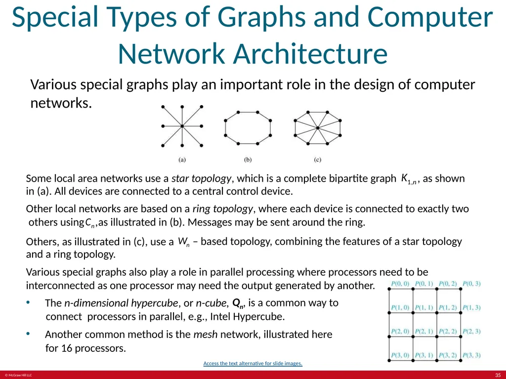
Special Types of Graphs and Computer Network Architecture Various special graphs play an important role in the design of computer networks. Some local area networks use a star topology, which is a complete bipartite graph , as shown in (a). All devices are connected to a central control device.
Other local networks are based on a ring topology, where each device is connected to exactly two others using ,as illustrated in (b). Messages may be sent around the ring. Others, as illustrated in (c), use a – based topology, combining the features of a star topology and a ring topology.
Various special graphs also play a role in parallel processing where processors need to be interconnected as one processor may need the output generated by another.
The n-dimensional hypercube, or n-cube, , is a common way to connect processors in parallel, e.g., Intel Hypercube. Another common method is the mesh network, illustrated here for 16 processors. Access the text alternative for slide images. 35<br>
Other local networks are based on a ring topology, where each device is connected to exactly two others using ,as illustrated in (b). Messages may be sent around the ring. Others, as illustrated in (c), use a – based topology, combining the features of a star topology and a ring topology.
Various special graphs also play a role in parallel processing where processors need to be interconnected as one processor may need the output generated by another.
The n-dimensional hypercube, or n-cube, , is a common way to connect processors in parallel, e.g., Intel Hypercube. Another common method is the mesh network, illustrated here for 16 processors. Access the text alternative for slide images. 35<br>
36
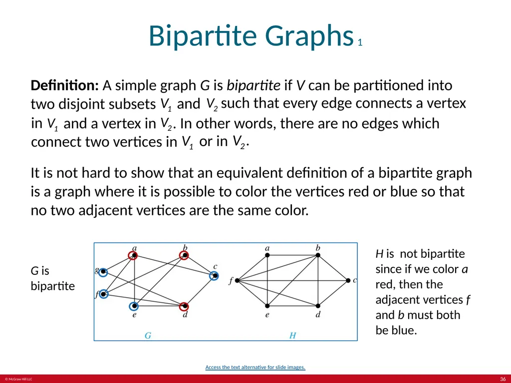
Bipartite Graphs 1 Definition: A simple graph G is bipartite if V can be partitioned into two disjoint subsets and such that every edge connects a vertex in and a vertex in . In other words, there are no edges which connect two vertices in or in It is not hard to show that an equivalent definition of a bipartite graph is a graph where it is possible to color the vertices red or blue so that no two adjacent vertices are the same color. G is bipartite H is not bipartite since if we color a red, then the adjacent vertices f and b must both be blue. Access the text alternative for slide images. 36<br>
37
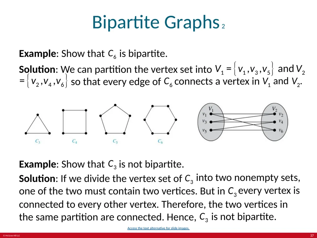
Bipartite Graphs 2 Example: Show that is bipartite. Solution: We can partition the vertex set into so that every edge of connects a vertex in Example: Show that is not bipartite. Solution: If we divide the vertex set of into two nonempty sets, one of the two must contain two vertices. But in every vertex is connected to every other vertex. Therefore, the two vertices in the same partition are connected. Hence, is not bipartite. Access the text alternative for slide images. 37<br>
38
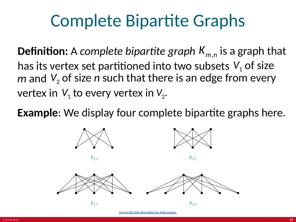
Complete Bipartite Graphs Definition: A complete bipartite graph is a graph that has its vertex set partitioned into two subsets of size m and of size n such that there is an edge from every vertex in to every vertex in Example: We display four complete bipartite graphs here. Access the text alternative for slide images. 38<br>
39
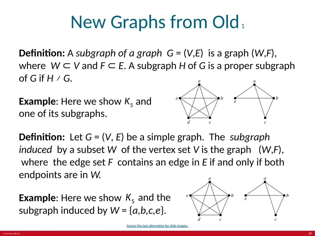
New Graphs from Old 1 Definition: A subgraph of a graph G = (V,E) is a graph (W,F), where W ⊂ V and F ⊂ E. A subgraph H of G is a proper subgraph of G if H ≠ G.
Example: Here we show and one of its subgraphs. Definition: Let G = (V, E) be a simple graph. The subgraph induced by a subset W of the vertex set V is the graph (W,F), where the edge set F contains an edge in E if and only if both endpoints are in W.
Example: Here we show and the subgraph induced by W = {a,b,c,e}. Access the text alternative for slide images. 39<br>
Example: Here we show and one of its subgraphs. Definition: Let G = (V, E) be a simple graph. The subgraph induced by a subset W of the vertex set V is the graph (W,F), where the edge set F contains an edge in E if and only if both endpoints are in W.
Example: Here we show and the subgraph induced by W = {a,b,c,e}. Access the text alternative for slide images. 39<br>
40
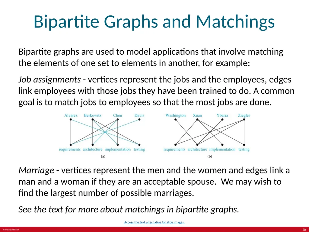
Bipartite Graphs and Matchings Bipartite graphs are used to model applications that involve matching the elements of one set to elements in another, for example:
Job assignments - vertices represent the jobs and the employees, edges link employees with those jobs they have been trained to do. A common goal is to match jobs to employees so that the most jobs are done. Marriage - vertices represent the men and the women and edges link a man and a woman if they are an acceptable spouse. We may wish to find the largest number of possible marriages.
See the text for more about matchings in bipartite graphs. Access the text alternative for slide images. 40<br>
Job assignments - vertices represent the jobs and the employees, edges link employees with those jobs they have been trained to do. A common goal is to match jobs to employees so that the most jobs are done. Marriage - vertices represent the men and the women and edges link a man and a woman if they are an acceptable spouse. We may wish to find the largest number of possible marriages.
See the text for more about matchings in bipartite graphs. Access the text alternative for slide images. 40<br>
41
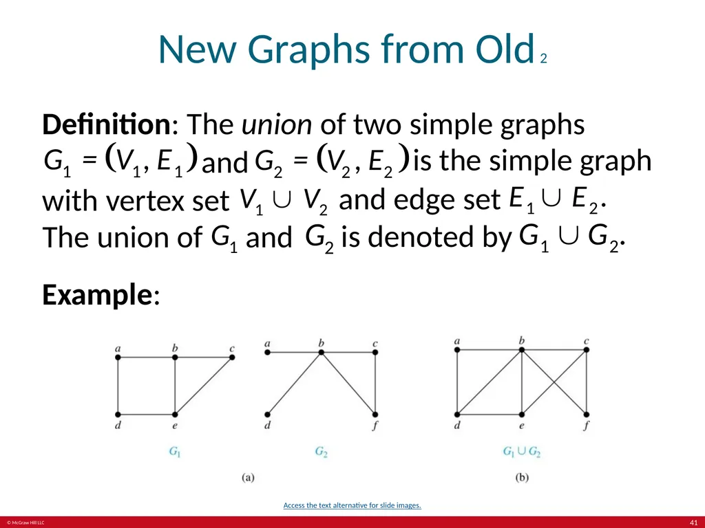
New Graphs from Old 2 Definition: The union of two simple graphs and is the simple graph with vertex set and edge set The union of and is denoted by Example: Access the text alternative for slide images. 41<br>
42
Representing Graphs and Graph Isomorphism Section 10.3 42<br>
43
Section Summary 3 Adjacency Lists.
Adjacency Matrices.
Incidence Matrices.
Isomorphism of Graphs. 43<br>
Adjacency Matrices.
Incidence Matrices.
Isomorphism of Graphs. 43<br>
44
Representing Graphs:
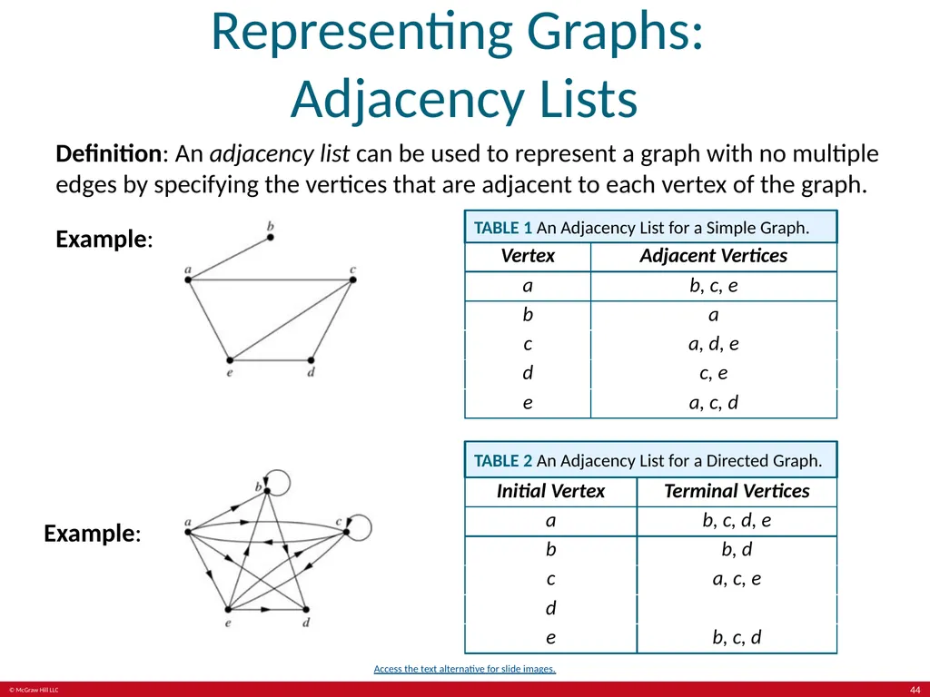
Adjacency Lists Definition: An adjacency list can be used to represent a graph with no multiple edges by specifying the vertices that are adjacent to each vertex of the graph.
Example: Example: TABLE 1 An Adjacency List for a Simple Graph. TABLE 2 An Adjacency List for a Directed Graph. For d there are no terminal vertices. Access the text alternative for slide images. 44<br>
Example: Example: TABLE 1 An Adjacency List for a Simple Graph. TABLE 2 An Adjacency List for a Directed Graph. For d there are no terminal vertices. Access the text alternative for slide images. 44<br>
45
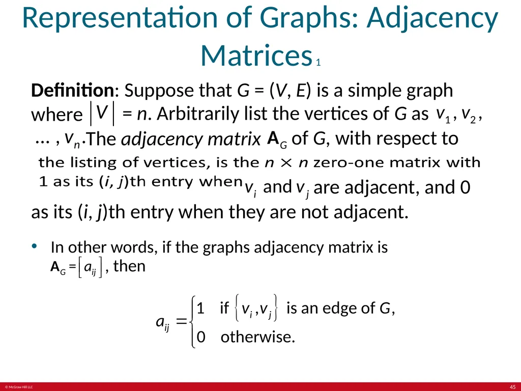
Representation of Graphs: Adjacency Matrices 1 Definition: Suppose that G = (V, E) is a simple graph where = n. Arbitrarily list the vertices of G as The adjacency matrix of G, with respect to are adjacent, and 0 as its (i, j)th entry when they are not adjacent.
In other words, if the graphs adjacency matrix is , then 45<br>
In other words, if the graphs adjacency matrix is , then 45<br>
46
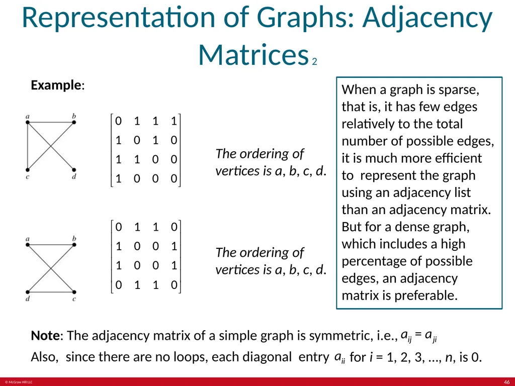
Representation of Graphs: Adjacency Matrices 2 Example: The ordering of vertices is a, b, c, d. The ordering of vertices is a, b, c, d. When a graph is sparse, that is, it has few edges relatively to the total number of possible edges, it is much more efficient to represent the graph using an adjacency list than an adjacency matrix. But for a dense graph, which includes a high percentage of possible edges, an adjacency matrix is preferable. Note: The adjacency matrix of a simple graph is symmetric, i.e., Also, since there are no loops, each diagonal entry for i = 1, 2, 3, …, n, is 0. 46<br>
47
Representation of Graphs: Adjacency Matrices 3 Adjacency matrices can also be used to represent graphs with loops and multiple edges.
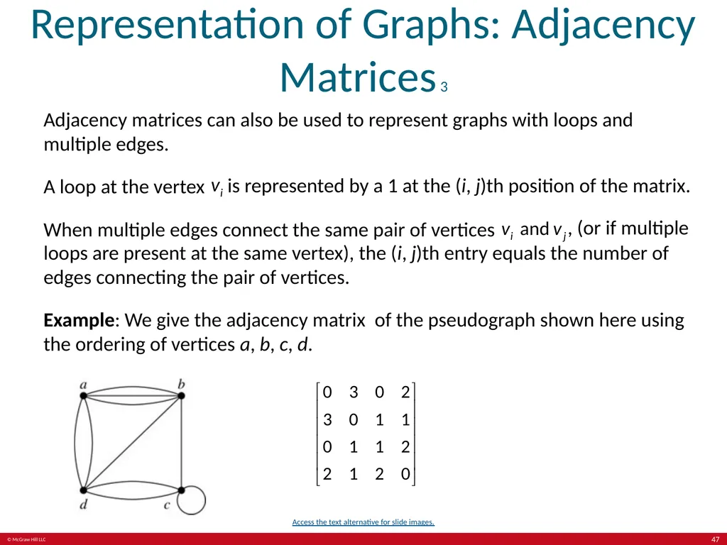
A loop at the vertex is represented by a 1 at the (i, j)th position of the matrix. When multiple edges connect the same pair of vertices , (or if multiple loops are present at the same vertex), the (i, j)th entry equals the number of edges connecting the pair of vertices.
Example: We give the adjacency matrix of the pseudograph shown here using the ordering of vertices a, b, c, d. Access the text alternative for slide images. 47<br>
A loop at the vertex is represented by a 1 at the (i, j)th position of the matrix. When multiple edges connect the same pair of vertices , (or if multiple loops are present at the same vertex), the (i, j)th entry equals the number of edges connecting the pair of vertices.
Example: We give the adjacency matrix of the pseudograph shown here using the ordering of vertices a, b, c, d. Access the text alternative for slide images. 47<br>
48
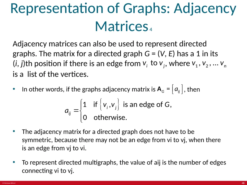
Representation of Graphs: Adjacency Matrices 4 Adjacency matrices can also be used to represent directed graphs. The matrix for a directed graph G = (V, E) has a 1 in its (i, j)th position if there is an edge from , where is a list of the vertices.
In other words, if the graphs adjacency matrix is , then The adjacency matrix for a directed graph does not have to be symmetric, because there may not be an edge from vi to vj, when there is an edge from vj to vi.
To represent directed multigraphs, the value of aij is the number of edges connecting vi to vj. 48<br>
In other words, if the graphs adjacency matrix is , then The adjacency matrix for a directed graph does not have to be symmetric, because there may not be an edge from vi to vj, when there is an edge from vj to vi.
To represent directed multigraphs, the value of aij is the number of edges connecting vi to vj. 48<br>
49
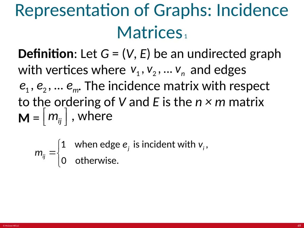
Representation of Graphs: Incidence Matrices 1 Definition: Let G = (V, E) be an undirected graph with vertices where and edges . The incidence matrix with respect to the ordering of V and E is the n × m matrix M = , where 49<br>
50
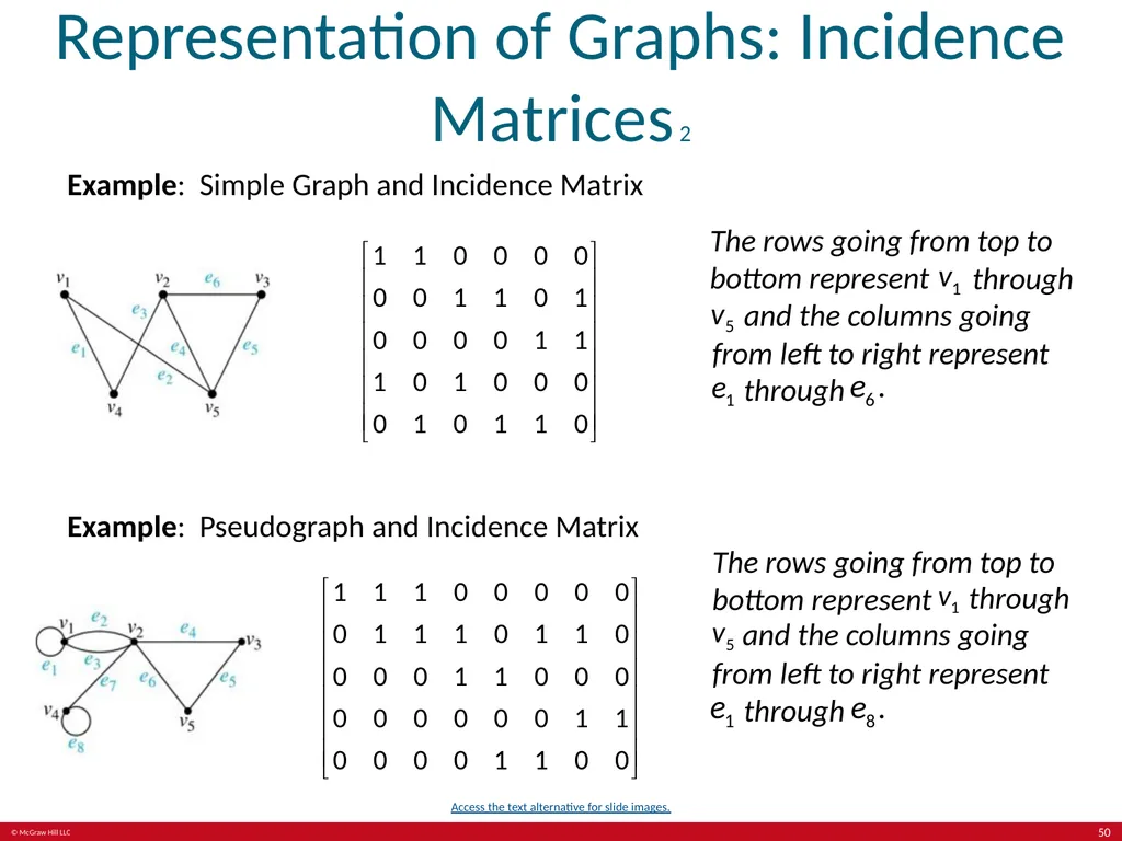
Representation of Graphs: Incidence Matrices 2 Example: Simple Graph and Incidence Matrix The rows going from top to bottom represent through and the columns going from left to right represent through Example: Pseudograph and Incidence Matrix The rows going from top to bottom represent through and the columns going from left to right represent through Access the text alternative for slide images. 50<br>
51
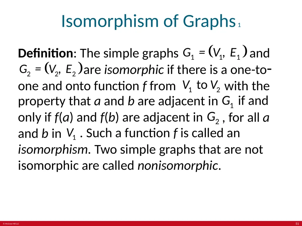
Isomorphism of Graphs 1 Definition: The simple graphs and are isomorphic if there is a one-to- one and onto function f from with the property that a and b are adjacent in if and only if f(a) and f(b) are adjacent in , for all a and b in . Such a function f is called an isomorphism. Two simple graphs that are not isomorphic are called nonisomorphic. 51<br>
52
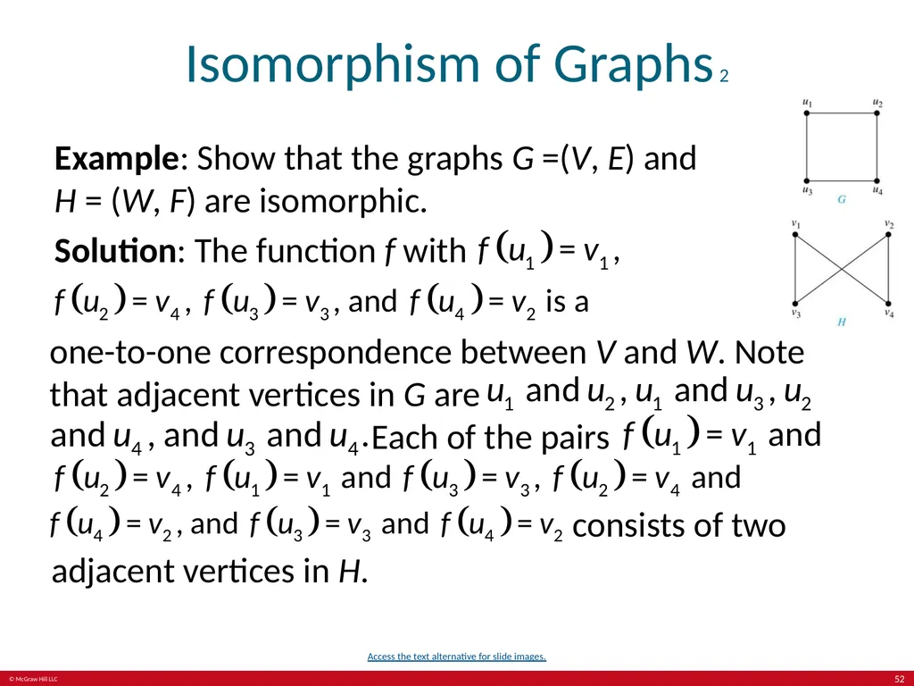
Isomorphism of Graphs 2 Example: Show that the graphs G =(V, E) and H = (W, F) are isomorphic.
Solution: The function f with one-to-one correspondence between V and W. Note that adjacent vertices in G are Each of the pairs consists of two adjacent vertices in H. Access the text alternative for slide images. 52<br>
Solution: The function f with one-to-one correspondence between V and W. Note that adjacent vertices in G are Each of the pairs consists of two adjacent vertices in H. Access the text alternative for slide images. 52<br>
53
Isomorphism of Graphs 3 It is difficult to determine whether two simple graphs are isomorphic using brute force because there are n possible one-to-one correspondences between the vertex sets of two simple graphs with n vertices.
The best algorithms for determining weather two graphs are isomorphic have exponential worst case complexity in terms of the number of vertices of the graphs.
Sometimes it is not hard to show that two graphs are not isomorphic. We can do so by finding a property, preserved by isomorphism, that only one of the two graphs has. Such a property is called graph invariant.
There are many different useful graph invariants that can be used to distinguish nonisomorphic graphs, such as the number of vertices, number of edges, and degree sequence (list of the degrees of the vertices in nonincreasing order). We will encounter others in later sections of this chapter. 53<br>
The best algorithms for determining weather two graphs are isomorphic have exponential worst case complexity in terms of the number of vertices of the graphs.
Sometimes it is not hard to show that two graphs are not isomorphic. We can do so by finding a property, preserved by isomorphism, that only one of the two graphs has. Such a property is called graph invariant.
There are many different useful graph invariants that can be used to distinguish nonisomorphic graphs, such as the number of vertices, number of edges, and degree sequence (list of the degrees of the vertices in nonincreasing order). We will encounter others in later sections of this chapter. 53<br>
54
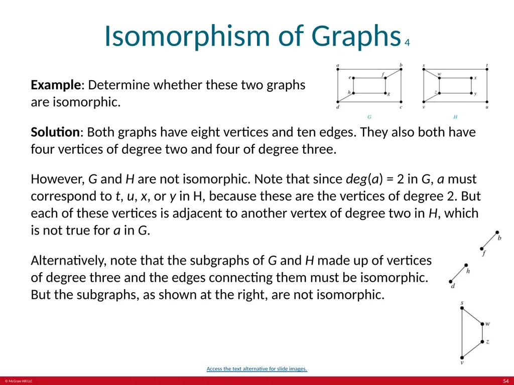
Isomorphism of Graphs 4 Example: Determine whether these two graphs
are isomorphic.
Solution: Both graphs have eight vertices and ten edges. They also both have four vertices of degree two and four of degree three.
However, G and H are not isomorphic. Note that since deg(a) = 2 in G, a must correspond to t, u, x, or y in H, because these are the vertices of degree 2. But each of these vertices is adjacent to another vertex of degree two in H, which is not true for a in G.
Alternatively, note that the subgraphs of G and H made up of vertices of degree three and the edges connecting them must be isomorphic. But the subgraphs, as shown at the right, are not isomorphic. Access the text alternative for slide images. 54<br>
Solution: Both graphs have eight vertices and ten edges. They also both have four vertices of degree two and four of degree three.
However, G and H are not isomorphic. Note that since deg(a) = 2 in G, a must correspond to t, u, x, or y in H, because these are the vertices of degree 2. But each of these vertices is adjacent to another vertex of degree two in H, which is not true for a in G.
Alternatively, note that the subgraphs of G and H made up of vertices of degree three and the edges connecting them must be isomorphic. But the subgraphs, as shown at the right, are not isomorphic. Access the text alternative for slide images. 54<br>
55
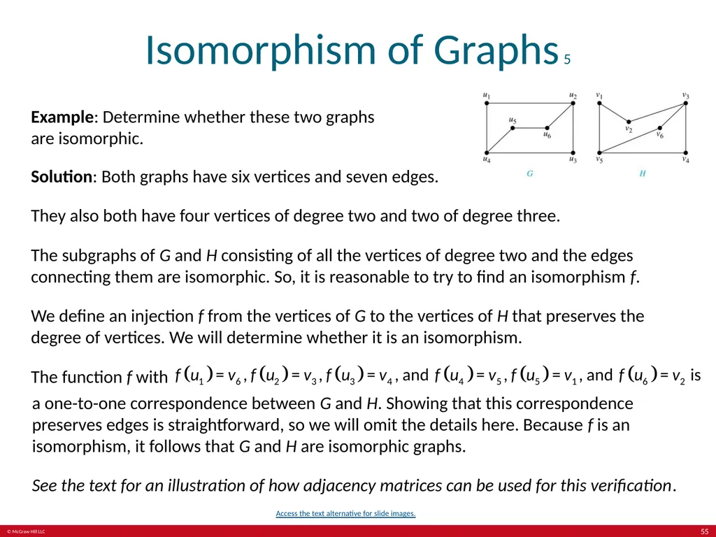
Isomorphism of Graphs 5 Example: Determine whether these two graphs are isomorphic. Solution: Both graphs have six vertices and seven edges.
They also both have four vertices of degree two and two of degree three.
The subgraphs of G and H consisting of all the vertices of degree two and the edges connecting them are isomorphic. So, it is reasonable to try to find an isomorphism f.
We define an injection f from the vertices of G to the vertices of H that preserves the degree of vertices. We will determine whether it is an isomorphism.
The function f with a one-to-one correspondence between G and H. Showing that this correspondence preserves edges is straightforward, so we will omit the details here. Because f is an isomorphism, it follows that G and H are isomorphic graphs.
See the text for an illustration of how adjacency matrices can be used for this verification. Access the text alternative for slide images. 55<br>
They also both have four vertices of degree two and two of degree three.
The subgraphs of G and H consisting of all the vertices of degree two and the edges connecting them are isomorphic. So, it is reasonable to try to find an isomorphism f.
We define an injection f from the vertices of G to the vertices of H that preserves the degree of vertices. We will determine whether it is an isomorphism.
The function f with a one-to-one correspondence between G and H. Showing that this correspondence preserves edges is straightforward, so we will omit the details here. Because f is an isomorphism, it follows that G and H are isomorphic graphs.
See the text for an illustration of how adjacency matrices can be used for this verification. Access the text alternative for slide images. 55<br>
56
Algorithms for Graph Isomorphism The best algorithms known for determining whether two graphs are isomorphic have exponential worst-case time complexity (in the number of vertices of the graphs).
However, there are algorithms with linear average-case time complexity.
You can use a public domain program called NAUTY to determine in less than a second whether two graphs with as many as 100 vertices are isomorphic.
Graph isomorphism is a problem of special interest because it is one of a few NP problems not known to be either tractable or NP-complete (see Section 3.3). 56<br>
However, there are algorithms with linear average-case time complexity.
You can use a public domain program called NAUTY to determine in less than a second whether two graphs with as many as 100 vertices are isomorphic.
Graph isomorphism is a problem of special interest because it is one of a few NP problems not known to be either tractable or NP-complete (see Section 3.3). 56<br>
57
Applications of Graph Isomorphism The question whether graphs are isomorphic plays an important role in applications of graph theory. For example,
chemists use molecular graphs to model chemical compounds. Vertices represent atoms and edges represent chemical bonds. When a new compound is synthesized, a database of molecular graphs is checked to determine whether the graph representing the new compound is isomorphic to the graph of a compound that this already known.
Electronic circuits are modeled as graphs in which the vertices represent components and the edges represent connections between them. Graph isomorphism is the basis for.
the verification that a particular layout of a circuit corresponds to the design’s original schematics.
determining whether a chip from one vendor includes the intellectual property of another vendor. 57<br>
chemists use molecular graphs to model chemical compounds. Vertices represent atoms and edges represent chemical bonds. When a new compound is synthesized, a database of molecular graphs is checked to determine whether the graph representing the new compound is isomorphic to the graph of a compound that this already known.
Electronic circuits are modeled as graphs in which the vertices represent components and the edges represent connections between them. Graph isomorphism is the basis for.
the verification that a particular layout of a circuit corresponds to the design’s original schematics.
determining whether a chip from one vendor includes the intellectual property of another vendor. 57<br>
58
Connectivity Section 10.4 58<br>
59
Section Summary 4 Paths.
Connectedness in Undirected Graphs.
Vertex Connectivity and Edge Connectivity (not currently included in overheads).
Connectedness in Directed Graphs.
Paths and Isomorphism (not currently included in overheads).
Counting Paths between Vertices. 59<br>
Connectedness in Undirected Graphs.
Vertex Connectivity and Edge Connectivity (not currently included in overheads).
Connectedness in Directed Graphs.
Paths and Isomorphism (not currently included in overheads).
Counting Paths between Vertices. 59<br>
60
Paths 1 Informal Definition: A path is a sequence of edges that begins at a vertex of a graph and travels from vertex to vertex along edges of the graph. As the path travels along its edges, it visits the vertices along this path, that is, the endpoints of these.
Applications: Numerous problems can be modeled with paths formed by traveling along edges of graphs such as:
determining whether a message can be sent between two computers.
efficiently planning routes for mail delivery. 60<br>
Applications: Numerous problems can be modeled with paths formed by traveling along edges of graphs such as:
determining whether a message can be sent between two computers.
efficiently planning routes for mail delivery. 60<br>
61
Paths 2 Definition: Let n be a nonnegative integer and G an undirected graph. A path of length n from u to v in G is a sequence of n edges of G for which there exists a sequence = v of vertices such that has, for i = the endpoints When the graph is simple, we denote this path by its vertex sequence (since listing the vertices uniquely determines the path). The path is a circuit if it begins and ends at the same vertex (u = v) and has length greater than zero.
The path or circuit is said to pass through the vertices and traverse the edges A path or circuit is simple if it does not contain the same edge more than once. This terminology is readily extended to directed graphs. (see text) 61<br>
The path or circuit is said to pass through the vertices and traverse the edges A path or circuit is simple if it does not contain the same edge more than once. This terminology is readily extended to directed graphs. (see text) 61<br>
62
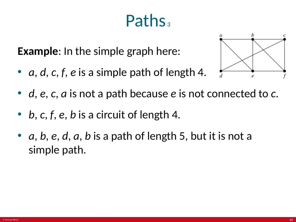
Paths 3 Example: In the simple graph here:
a, d, c, f, e is a simple path of length 4.
d, e, c, a is not a path because e is not connected to c.
b, c, f, e, b is a circuit of length 4.
a, b, e, d, a, b is a path of length 5, but it is not a simple path. 62<br>
a, d, c, f, e is a simple path of length 4.
d, e, c, a is not a path because e is not connected to c.
b, c, f, e, b is a circuit of length 4.
a, b, e, d, a, b is a path of length 5, but it is not a simple path. 62<br>
63
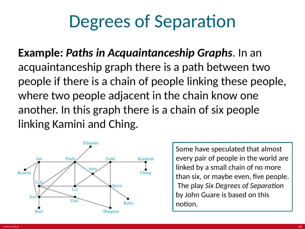
Degrees of Separation Example: Paths in Acquaintanceship Graphs. In an acquaintanceship graph there is a path between two people if there is a chain of people linking these people, where two people adjacent in the chain know one another. In this graph there is a chain of six people linking Kamini and Ching. Some have speculated that almost every pair of people in the world are linked by a small chain of no more than six, or maybe even, five people. The play Six Degrees of Separation by John Guare is based on this notion. 63<br>
64
Erdős numbers Paul Erdős Example: Erdős numbers.
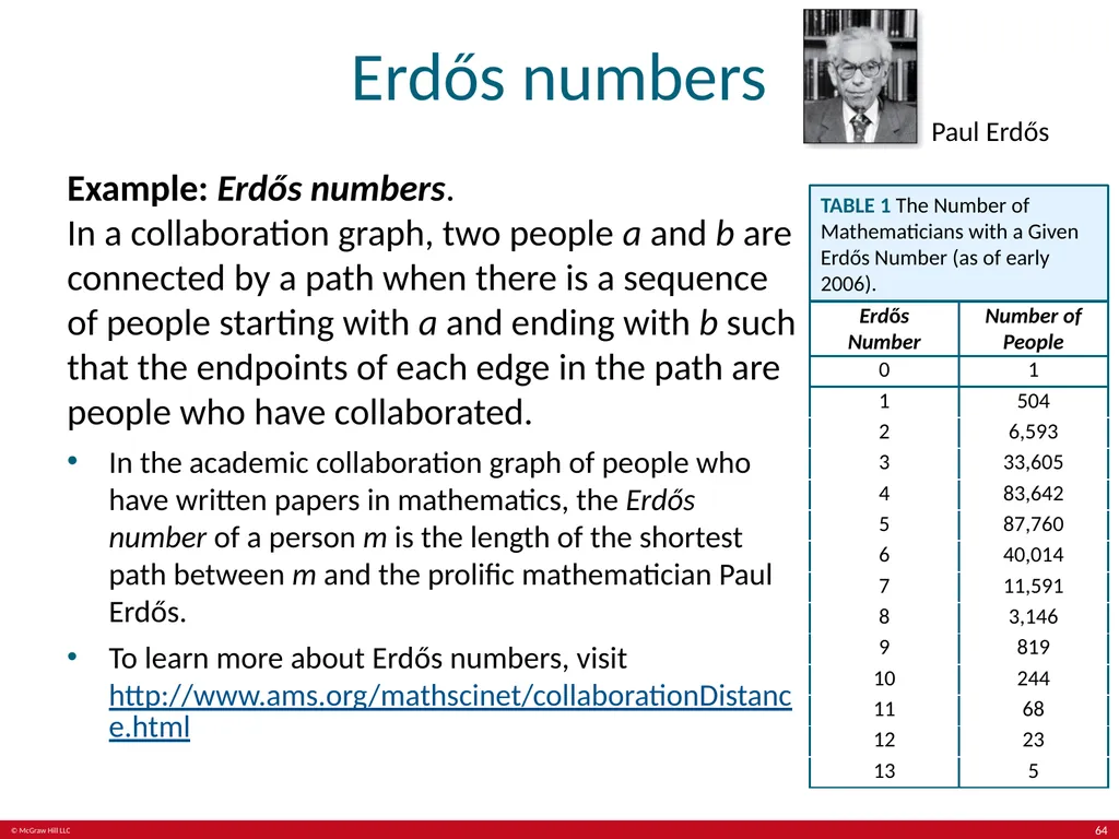
In a collaboration graph, two people a and b are connected by a path when there is a sequence of people starting with a and ending with b such that the endpoints of each edge in the path are people who have collaborated.
In the academic collaboration graph of people who have written papers in mathematics, the Erdős number of a person m is the length of the shortest path between m and the prolific mathematician Paul Erdős.
To learn more about Erdős numbers, visit http://www.ams.org/mathscinet/collaborationDistance.html TABLE 1 The Number of Mathematicians with a Given Erdős Number (as of early 2006). 64<br>
In the academic collaboration graph of people who have written papers in mathematics, the Erdős number of a person m is the length of the shortest path between m and the prolific mathematician Paul Erdős.
To learn more about Erdős numbers, visit http://www.ams.org/mathscinet/collaborationDistance.html TABLE 1 The Number of Mathematicians with a Given Erdős Number (as of early 2006). 64<br>
65
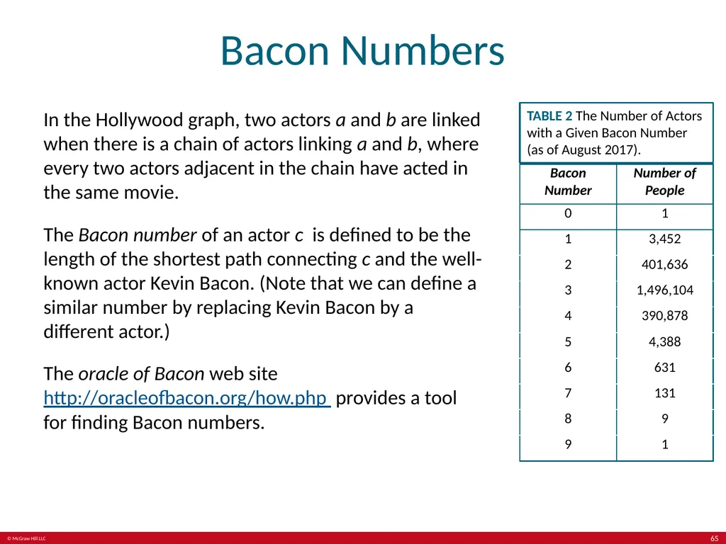
Bacon Numbers In the Hollywood graph, two actors a and b are linked when there is a chain of actors linking a and b, where every two actors adjacent in the chain have acted in the same movie.
The Bacon number of an actor c is defined to be the length of the shortest path connecting c and the well-known actor Kevin Bacon. (Note that we can define a similar number by replacing Kevin Bacon by a different actor.)
The oracle of Bacon web site http://oracleofbacon.org/how.php provides a tool for finding Bacon numbers. TABLE 2 The Number of Actors with a Given Bacon Number (as of August 2017). 65<br>
The Bacon number of an actor c is defined to be the length of the shortest path connecting c and the well-known actor Kevin Bacon. (Note that we can define a similar number by replacing Kevin Bacon by a different actor.)
The oracle of Bacon web site http://oracleofbacon.org/how.php provides a tool for finding Bacon numbers. TABLE 2 The Number of Actors with a Given Bacon Number (as of August 2017). 65<br>
66
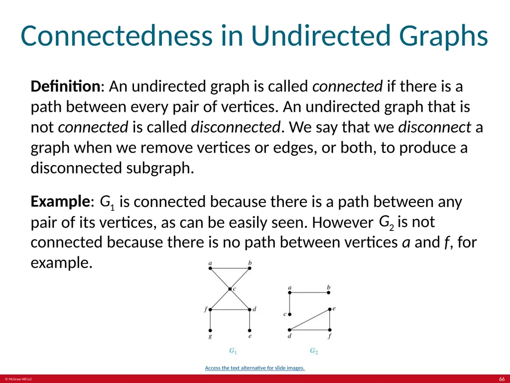
Connectedness in Undirected Graphs Definition: An undirected graph is called connected if there is a path between every pair of vertices. An undirected graph that is not connected is called disconnected. We say that we disconnect a graph when we remove vertices or edges, or both, to produce a disconnected subgraph.
Example: is connected because there is a path between any pair of its vertices, as can be easily seen. However is not connected because there is no path between vertices a and f, for example. Access the text alternative for slide images. 66<br>
Example: is connected because there is a path between any pair of its vertices, as can be easily seen. However is not connected because there is no path between vertices a and f, for example. Access the text alternative for slide images. 66<br>
67
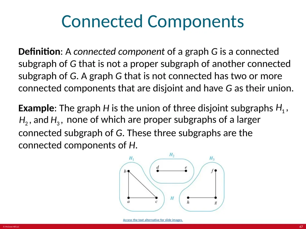
Connected Components Definition: A connected component of a graph G is a connected subgraph of G that is not a proper subgraph of another connected subgraph of G. A graph G that is not connected has two or more connected components that are disjoint and have G as their union.
Example: The graph H is the union of three disjoint subgraphs none of which are proper subgraphs of a larger connected subgraph of G. These three subgraphs are the connected components of H. Access the text alternative for slide images. 67<br>
Example: The graph H is the union of three disjoint subgraphs none of which are proper subgraphs of a larger connected subgraph of G. These three subgraphs are the connected components of H. Access the text alternative for slide images. 67<br>
68
Connectedness in Directed Graphs 1 Definition: A directed graph is strongly connected if there is a path from a to b and a path from b to a whenever a and b are vertices in the graph.
Definition: A directed graph is weakly connected if there is a path between every two vertices in the underlying undirected graph, which is the undirected graph obtained by ignoring the directions of the edges of the directed graph. 68<br>
Definition: A directed graph is weakly connected if there is a path between every two vertices in the underlying undirected graph, which is the undirected graph obtained by ignoring the directions of the edges of the directed graph. 68<br>
69
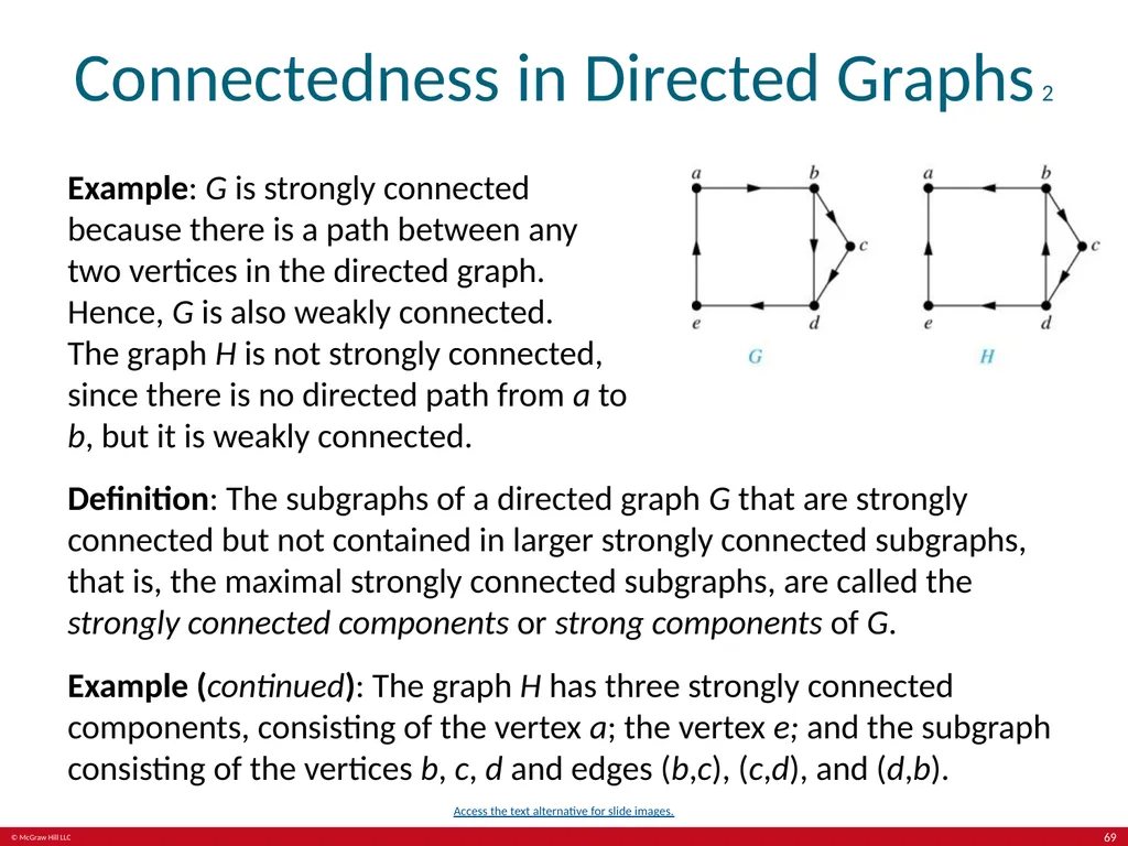
Connectedness in Directed Graphs 2 Example: G is strongly connected because there is a path between any two vertices in the directed graph. Hence, G is also weakly connected.
The graph H is not strongly connected, since there is no directed path from a to b, but it is weakly connected. Definition: The subgraphs of a directed graph G that are strongly connected but not contained in larger strongly connected subgraphs, that is, the maximal strongly connected subgraphs, are called the strongly connected components or strong components of G.
Example (continued): The graph H has three strongly connected components, consisting of the vertex a; the vertex e; and the subgraph consisting of the vertices b, c, d and edges (b,c), (c,d), and (d,b). Access the text alternative for slide images. 69<br>
Example (continued): The graph H has three strongly connected components, consisting of the vertex a; the vertex e; and the subgraph consisting of the vertices b, c, d and edges (b,c), (c,d), and (d,b). Access the text alternative for slide images. 69<br>
70
The Connected Components of the Web Graph Recall that at any particular instant the web graph provides a snapshot of the web, where vertices represent web pages and edges represent links. According to a 1999 study, the Web graph at that time had over 200 million vertices and over 1.5 billion edges. (The numbers today are several orders of magnitude larger.)
The underlying undirected graph of this Web graph has a connected component that includes approximately 90% of the vertices.
There is a giant strongly connected component (GSCC) consisting of more than 53 million vertices. A Web page in this component can be reached by following links starting in any other page of the component. There are three other categories of pages with each having about 44 million vertices:
pages that can be reached from a page in the GSCC, but do not link back.
pages that link back to the GSCC, but can not be reached by following links from pages in the GSCC.
pages that cannot reach pages in the GSCC and can not be reached from pages in the GSCC. 70<br>
The underlying undirected graph of this Web graph has a connected component that includes approximately 90% of the vertices.
There is a giant strongly connected component (GSCC) consisting of more than 53 million vertices. A Web page in this component can be reached by following links starting in any other page of the component. There are three other categories of pages with each having about 44 million vertices:
pages that can be reached from a page in the GSCC, but do not link back.
pages that link back to the GSCC, but can not be reached by following links from pages in the GSCC.
pages that cannot reach pages in the GSCC and can not be reached from pages in the GSCC. 70<br>
71
Counting Paths between Vertices 1 We can use the adjacency matrix of a graph to find the number of paths between two vertices in the graph.
Theorem: Let G be a graph with adjacency matrix A with respect to the ordering of vertices (with directed or undirected edges, multiple edges and loops allowed). The number of different paths of length r from , where r >0 is a positive integer, equals the (i,j)th entry of Proof by mathematical induction:
Basis Step: By definition of the adjacency matrix, the number of paths from length 1 is the (i,j)th entry of A.
Inductive Step: For the inductive hypothesis, we assume that that the (i,j)th entry of is the number of different paths of length r from Because , the (i,j)th entry of (i,k)th entry of By the inductive hypothesis, is the number of paths of length r from A path of length r + 1 from is made up of a path of length r from to some , and an edge from By the product rule for counting, the number of such paths is the product of the number of paths of length r from and the number of edges from The sum over all possible intermediate vertices 71<br>
Theorem: Let G be a graph with adjacency matrix A with respect to the ordering of vertices (with directed or undirected edges, multiple edges and loops allowed). The number of different paths of length r from , where r >0 is a positive integer, equals the (i,j)th entry of Proof by mathematical induction:
Basis Step: By definition of the adjacency matrix, the number of paths from length 1 is the (i,j)th entry of A.
Inductive Step: For the inductive hypothesis, we assume that that the (i,j)th entry of is the number of different paths of length r from Because , the (i,j)th entry of (i,k)th entry of By the inductive hypothesis, is the number of paths of length r from A path of length r + 1 from is made up of a path of length r from to some , and an edge from By the product rule for counting, the number of such paths is the product of the number of paths of length r from and the number of edges from The sum over all possible intermediate vertices 71<br>
72
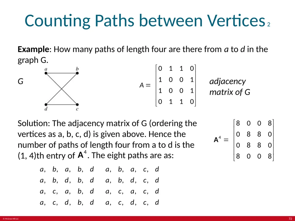
Counting Paths between Vertices 2 Example: How many paths of length four are there from a to d in the graph G. G adjacency matrix of G Solution: The adjacency matrix of G (ordering the vertices as a, b, c, d) is given above. Hence the number of paths of length four from a to d is the (1, 4)th entry of . The eight paths are as: 72<br>
73
Euler and Hamiltonian Graphs Section 10.5 73<br>
74
Section Summary 5 Euler Paths and Circuits.
Hamilton Paths and Circuits.
Applications of Hamilton Circuits. 74<br>
Hamilton Paths and Circuits.
Applications of Hamilton Circuits. 74<br>
75
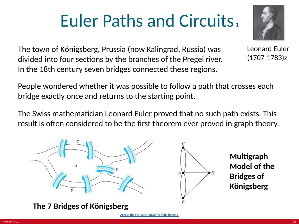
Euler Paths and Circuits 1 Leonard Euler (1707-1783)z The town of Kӧnigsberg, Prussia (now Kalingrad, Russia) was divided into four sections by the branches of the Pregel river. In the 18th century seven bridges connected these regions. People wondered whether it was possible to follow a path that crosses each bridge exactly once and returns to the starting point.
The Swiss mathematician Leonard Euler proved that no such path exists. This result is often considered to be the first theorem ever proved in graph theory. The 7 Bridges of Kӧnigsberg Multigraph Model of the Bridges of Kӧnigsberg Access the text alternative for slide images. 75<br>
The Swiss mathematician Leonard Euler proved that no such path exists. This result is often considered to be the first theorem ever proved in graph theory. The 7 Bridges of Kӧnigsberg Multigraph Model of the Bridges of Kӧnigsberg Access the text alternative for slide images. 75<br>
76
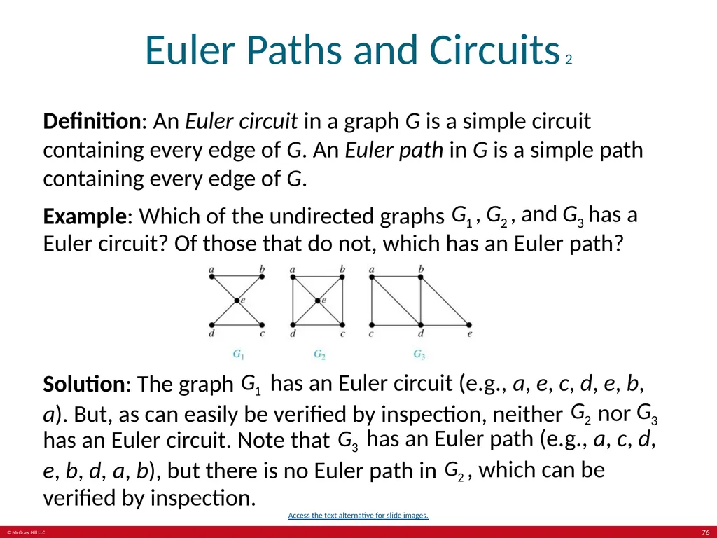
Euler Paths and Circuits 2 Definition: An Euler circuit in a graph G is a simple circuit containing every edge of G. An Euler path in G is a simple path containing every edge of G.
Example: Which of the undirected graphs has a Euler circuit? Of those that do not, which has an Euler path? Solution: The graph has an Euler circuit (e.g., a, e, c, d, e, b, a). But, as can easily be verified by inspection, neither nor has an Euler circuit. Note that has an Euler path (e.g., a, c, d, e, b, d, a, b), but there is no Euler path in , which can be verified by inspection. Access the text alternative for slide images. 76<br>
Example: Which of the undirected graphs has a Euler circuit? Of those that do not, which has an Euler path? Solution: The graph has an Euler circuit (e.g., a, e, c, d, e, b, a). But, as can easily be verified by inspection, neither nor has an Euler circuit. Note that has an Euler path (e.g., a, c, d, e, b, d, a, b), but there is no Euler path in , which can be verified by inspection. Access the text alternative for slide images. 76<br>
77
Necessary Conditions for Euler Circuits and Paths An Euler circuit begins with a vertex a and continues with an edge incident with a, say {a, b}. The edge {a, b} contributes one to deg(a).
Each time the circuit passes through a vertex it contributes two to the vertex’s degree.
Finally, the circuit terminates where it started, contributing one to deg(a). Therefore deg(a) must be even.
We conclude that the degree of every other vertex must also be even.
By the same reasoning, we see that the initial vertex and the final vertex of an Euler path have odd degree, while every other vertex has even degree. So, a graph with an Euler path has exactly two vertices of odd degree.
In the next slide we will show that these necessary conditions are also sufficient conditions. 77<br>
Each time the circuit passes through a vertex it contributes two to the vertex’s degree.
Finally, the circuit terminates where it started, contributing one to deg(a). Therefore deg(a) must be even.
We conclude that the degree of every other vertex must also be even.
By the same reasoning, we see that the initial vertex and the final vertex of an Euler path have odd degree, while every other vertex has even degree. So, a graph with an Euler path has exactly two vertices of odd degree.
In the next slide we will show that these necessary conditions are also sufficient conditions. 77<br>
78
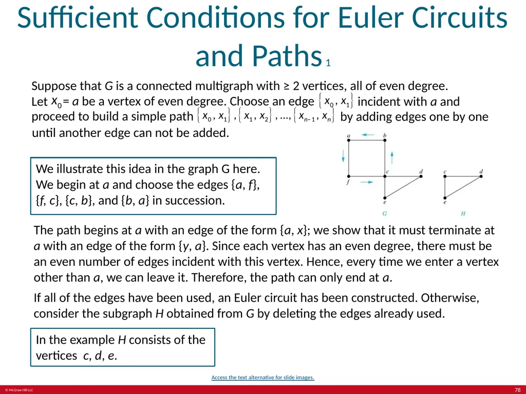
Sufficient Conditions for Euler Circuits and Paths 1 Suppose that G is a connected multigraph with ≥ 2 vertices, all of even degree.
Let = a be a vertex of even degree. Choose an edge incident with a and proceed to build a simple path by adding edges one by one until another edge can not be added. We illustrate this idea in the graph G here. We begin at a and choose the edges {a, f}, {f, c}, {c, b}, and {b, a} in succession. The path begins at a with an edge of the form {a, x}; we show that it must terminate at a with an edge of the form {y, a}. Since each vertex has an even degree, there must be an even number of edges incident with this vertex. Hence, every time we enter a vertex other than a, we can leave it. Therefore, the path can only end at a.
If all of the edges have been used, an Euler circuit has been constructed. Otherwise, consider the subgraph H obtained from G by deleting the edges already used. In the example H consists of the vertices c, d, e. Access the text alternative for slide images. 78<br>
If all of the edges have been used, an Euler circuit has been constructed. Otherwise, consider the subgraph H obtained from G by deleting the edges already used. In the example H consists of the vertices c, d, e. Access the text alternative for slide images. 78<br>
79
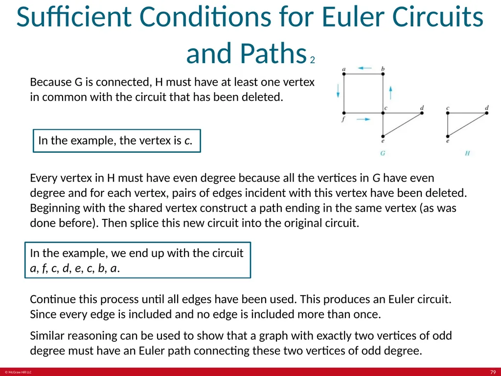
Sufficient Conditions for Euler Circuits and Paths 2 Because G is connected, H must have at least one vertex
in common with the circuit that has been deleted. In the example, the vertex is c. Every vertex in H must have even degree because all the vertices in G have even degree and for each vertex, pairs of edges incident with this vertex have been deleted. Beginning with the shared vertex construct a path ending in the same vertex (as was done before). Then splice this new circuit into the original circuit. In the example, we end up with the circuit a, f, c, d, e, c, b, a. Continue this process until all edges have been used. This produces an Euler circuit. Since every edge is included and no edge is included more than once.
Similar reasoning can be used to show that a graph with exactly two vertices of odd degree must have an Euler path connecting these two vertices of odd degree. 79<br>
Similar reasoning can be used to show that a graph with exactly two vertices of odd degree must have an Euler path connecting these two vertices of odd degree. 79<br>
80
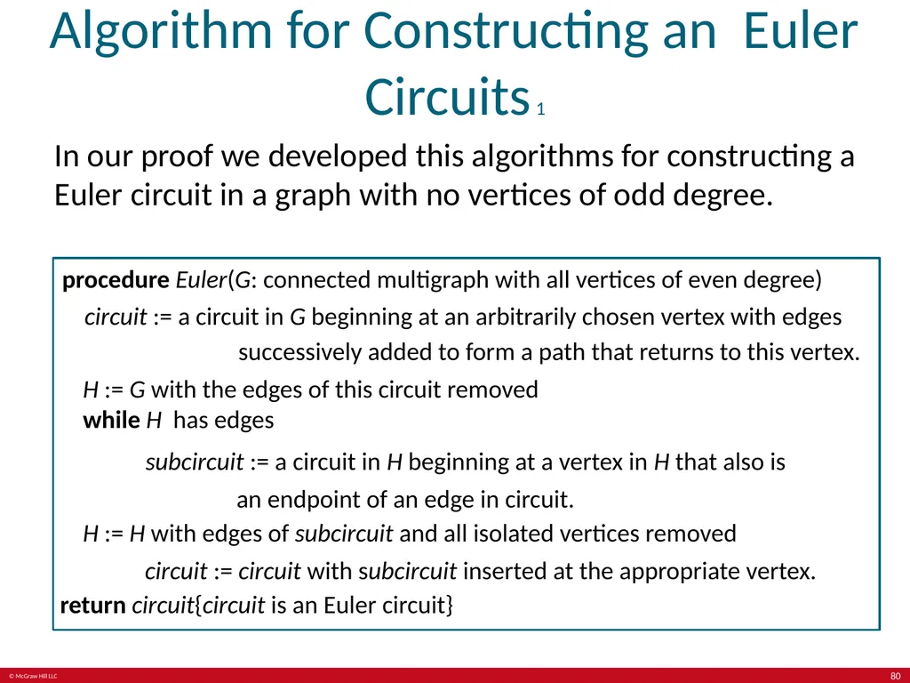
Algorithm for Constructing an Euler Circuits 1 In our proof we developed this algorithms for constructing a Euler circuit in a graph with no vertices of odd degree. procedure Euler(G: connected multigraph with all vertices of even degree) circuit := a circuit in G beginning at an arbitrarily chosen vertex with edges successively added to form a path that returns to this vertex. H := G with the edges of this circuit removed while H has edges subcircuit := a circuit in H beginning at a vertex in H that also is an endpoint of an edge in circuit. H := H with edges of subcircuit and all isolated vertices removed circuit := circuit with subcircuit inserted at the appropriate vertex. return circuit{circuit is an Euler circuit} 80<br>
81
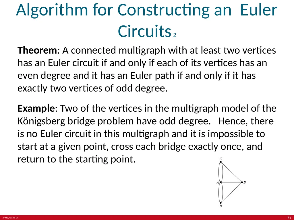
Algorithm for Constructing an Euler Circuits 2 Theorem: A connected multigraph with at least two vertices has an Euler circuit if and only if each of its vertices has an even degree and it has an Euler path if and only if it has exactly two vertices of odd degree.
Example: Two of the vertices in the multigraph model of the Kӧnigsberg bridge problem have odd degree. Hence, there is no Euler circuit in this multigraph and it is impossible to start at a given point, cross each bridge exactly once, and return to the starting point. 81<br>
Example: Two of the vertices in the multigraph model of the Kӧnigsberg bridge problem have odd degree. Hence, there is no Euler circuit in this multigraph and it is impossible to start at a given point, cross each bridge exactly once, and return to the starting point. 81<br>
82
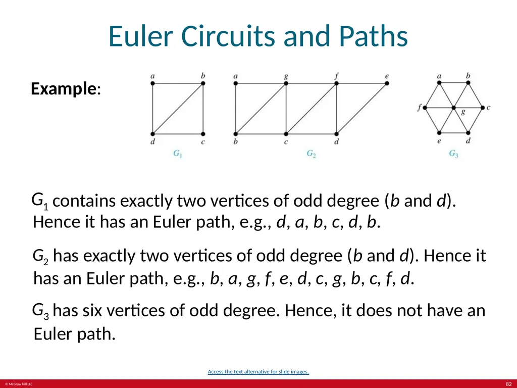
Euler Circuits and Paths Example: contains exactly two vertices of odd degree (b and d). Hence it has an Euler path, e.g., d, a, b, c, d, b. has exactly two vertices of odd degree (b and d). Hence it has an Euler path, e.g., b, a, g, f, e, d, c, g, b, c, f, d. has six vertices of odd degree. Hence, it does not have an Euler path. Access the text alternative for slide images. 82<br>
83
Applications of Euler Paths and Circuits Euler paths and circuits can be used to solve many practical problems such as finding a path or circuit that traverses each
street in a neighborhood,
road in a transportation network,
connection in a utility grid,
link in a communications network.
Other applications are found in the
layout of circuits,
network multicasting,
molecular biology, where Euler paths are used in the sequencing of DNA. 83<br>
street in a neighborhood,
road in a transportation network,
connection in a utility grid,
link in a communications network.
Other applications are found in the
layout of circuits,
network multicasting,
molecular biology, where Euler paths are used in the sequencing of DNA. 83<br>
84
Hamilton Paths and Circuits 1 William Rowan Hamilton (1805- 1865) Euler paths and circuits contained every edge only once.
Now we look at paths and circuits that contain every vertex exactly once. William Hamilton invented the Icosian puzzle in 1857.
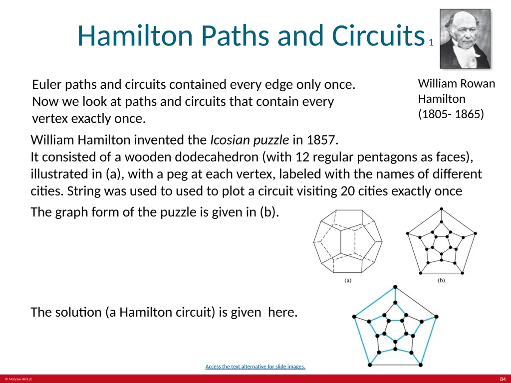
It consisted of a wooden dodecahedron (with 12 regular pentagons as faces), illustrated in (a), with a peg at each vertex, labeled with the names of different cities. String was used to used to plot a circuit visiting 20 cities exactly once
The graph form of the puzzle is given in (b). The solution (a Hamilton circuit) is given here. Access the text alternative for slide images. 84<br>
The graph form of the puzzle is given in (b). The solution (a Hamilton circuit) is given here. Access the text alternative for slide images. 84<br>
85
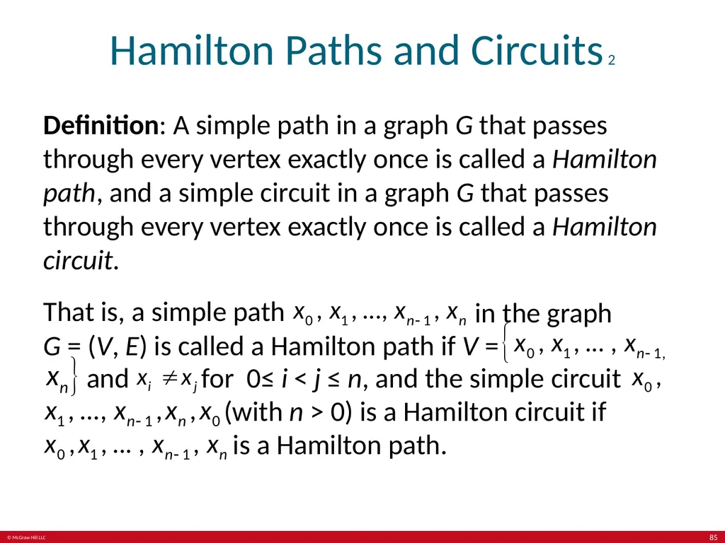
Hamilton Paths and Circuits 2 Definition: A simple path in a graph G that passes through every vertex exactly once is called a Hamilton path, and a simple circuit in a graph G that passes through every vertex exactly once is called a Hamilton circuit.
That is, a simple path in the graph G = (V, E) is called a Hamilton path if V = and for 0≤ i < j ≤ n, and the simple circuit (with n > 0) is a Hamilton circuit if is a Hamilton path. 85<br>
That is, a simple path in the graph G = (V, E) is called a Hamilton path if V = and for 0≤ i < j ≤ n, and the simple circuit (with n > 0) is a Hamilton circuit if is a Hamilton path. 85<br>
86
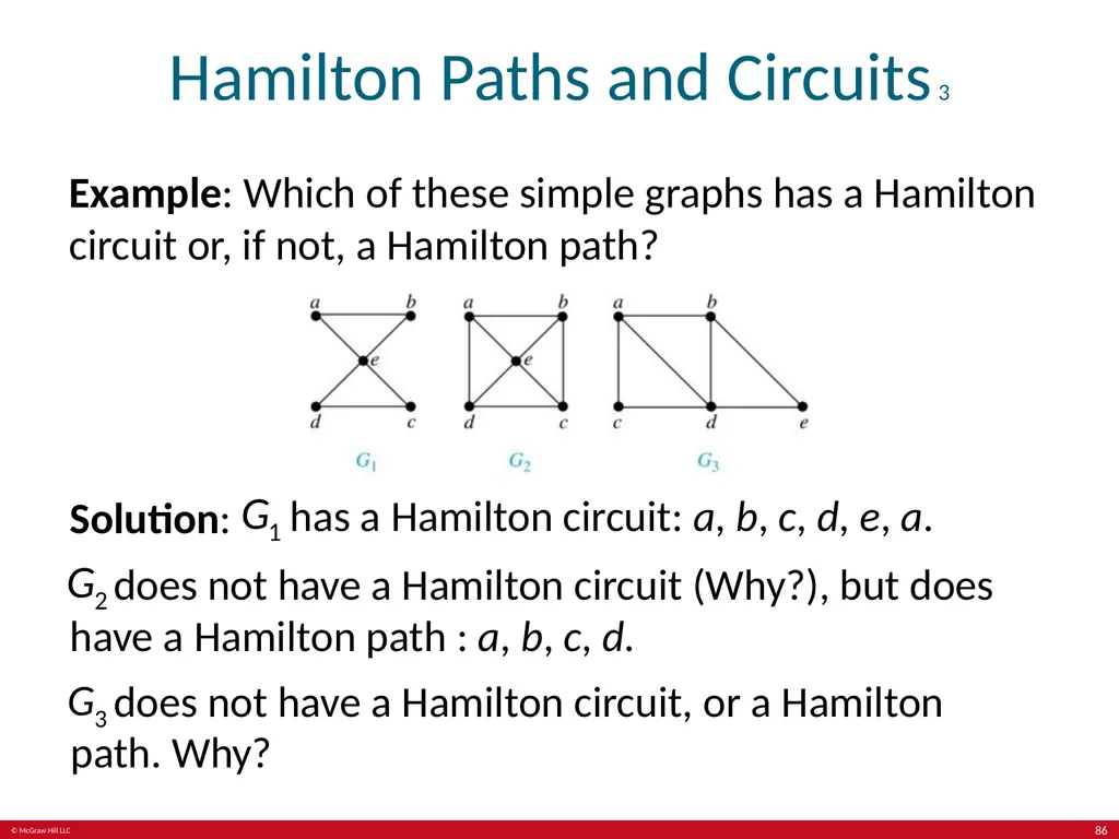
Hamilton Paths and Circuits 3 Example: Which of these simple graphs has a Hamilton circuit or, if not, a Hamilton path? Solution: has a Hamilton circuit: a, b, c, d, e, a. does not have a Hamilton circuit (Why?), but does have a Hamilton path : a, b, c, d. does not have a Hamilton circuit, or a Hamilton path. Why? 86<br>
87
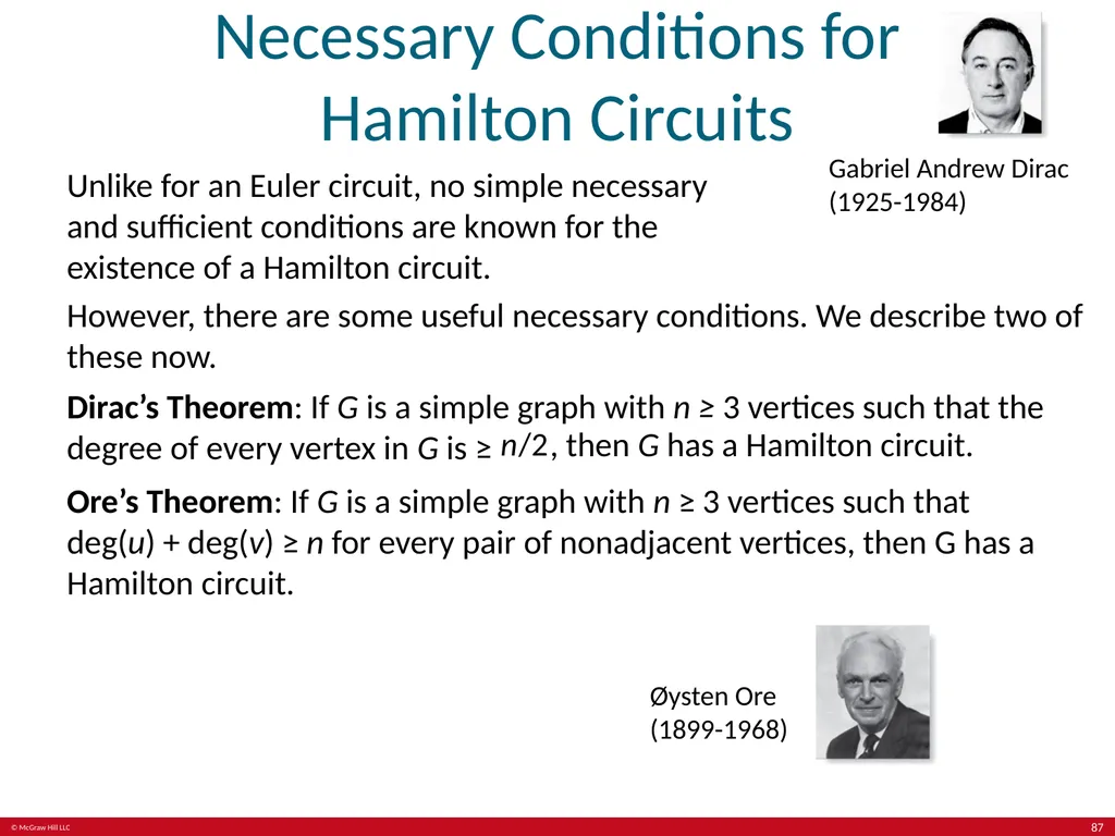
Necessary Conditions for Hamilton Circuits Gabriel Andrew Dirac (1925-1984) Unlike for an Euler circuit, no simple necessary and sufficient conditions are known for the existence of a Hamilton circuit. However, there are some useful necessary conditions. We describe two of these now.
Dirac’s Theorem: If G is a simple graph with n ≥ 3 vertices such that the degree of every vertex in G is ≥ , then G has a Hamilton circuit. Ore’s Theorem: If G is a simple graph with n ≥ 3 vertices such that deg(u) + deg(v) ≥ n for every pair of nonadjacent vertices, then G has a Hamilton circuit. Øysten Ore (1899-1968) 87<br>
Dirac’s Theorem: If G is a simple graph with n ≥ 3 vertices such that the degree of every vertex in G is ≥ , then G has a Hamilton circuit. Ore’s Theorem: If G is a simple graph with n ≥ 3 vertices such that deg(u) + deg(v) ≥ n for every pair of nonadjacent vertices, then G has a Hamilton circuit. Øysten Ore (1899-1968) 87<br>
88
Applications of Hamilton Paths and Circuits Applications that ask for a path or a circuit that visits each intersection of a city, each place pipelines intersect in a utility grid, or each node in a communications network exactly once, can be solved by finding a Hamilton path in the appropriate graph.
The famous traveling salesperson problem (TSP) asks for the shortest route a traveling salesperson should take to visit a set of cities. This problem reduces to finding a Hamilton circuit such that the total sum of the weights of its edges is as small as possible.
A family of binary codes, known as Gray codes, which minimize the effect of transmission errors, correspond to Hamilton circuits in the n-cube (See the text for details.) 88<br>
The famous traveling salesperson problem (TSP) asks for the shortest route a traveling salesperson should take to visit a set of cities. This problem reduces to finding a Hamilton circuit such that the total sum of the weights of its edges is as small as possible.
A family of binary codes, known as Gray codes, which minimize the effect of transmission errors, correspond to Hamilton circuits in the n-cube (See the text for details.) 88<br>
89
End of Main Content © McGraw Hill LLC. All rights reserved. No reproduction or distribution without the prior written consent of McGraw Hill LLC.<br>
90
Accessibility Content:
Text Alternatives for Images 90<br>
91
Some Terminology 1 – Text Alternative Return to parent-slide containing images. a is connected to c and b is connected to c by a curve each. c has an oval and b has an oval touching the circle. Return to parent-slide containing images. 91<br>
92
Some Terminology 2 – Text Alternative Return to parent-slide containing images. (Top Image) Three circles a, b, and c forming a triangle are above three circles ab, and c forming a triangle. a is connected to b and c. b is connected to c. c is connected to a. Return to parent-slide containing images. 92<br>
93
Graph Models:
Computer Networks 1 – Text Alternative Return to parent-slide containing images. The vertices are San Francisco, Los Angeles, Denver. Chicago, Detroit, New York, and Washington. The edges are from San Francisco to Los Angeles, from San Francisco to Denver, from Los Angeles to Denver. From Denver to Chicago, from Chicago to Detroit, from Chicago to Washington. From Chicago to New York. From Detroit to New York, and from Washington to New York. Return to parent-slide containing images. 93<br>
94
Graph Models:
Computer Networks 2 – Text Alternative Return to parent-slide containing images. (Top Image) 2 edges between Los Angeles and Denver, 3 edges between Denver and Chicago, 2 edges between Chicago and New York, and 2 edges between New York and Washington.
(Middle Image) The vertices are San Francisco, Los Angeles, Denver. Chicago, Detroit, New York, and Washington. The edges are directed from San Francisco to Los Angeles, from San Francisco to Denver. From Los Angeles to Denver, from Denver to Los Angeles. From Denver to Chicago, from Chicago to Denver. From Chicago to Detroit, from Detroit to Chicago. From Chicago to Washington, from Washington to Chicago. From Chicago to New York, from Detroit to New York, and from Washington to New York.
(Bottom Image) The vertices are San Francisco, Los Angeles, Denver. Chicago, Detroit, New York, and Washington. The edges are directed from San Francisco to Los Angeles, from Los Angeles to San Francisco. 2 from San Francisco to Denver, from Denver to San Francisco. From Los Angeles to Denver, from Denver to Los Angeles. 2 from Denver to Chicago, 2 from Chicago to Denver. From Chicago to Detroit, from Detroit to New York, 2 from Chicago to New York. From Chicago to Washington, from Washington to Chicago. And 2 from Washington to New York. Return to parent-slide containing images. 94<br>
(Middle Image) The vertices are San Francisco, Los Angeles, Denver. Chicago, Detroit, New York, and Washington. The edges are directed from San Francisco to Los Angeles, from San Francisco to Denver. From Los Angeles to Denver, from Denver to Los Angeles. From Denver to Chicago, from Chicago to Denver. From Chicago to Detroit, from Detroit to Chicago. From Chicago to Washington, from Washington to Chicago. From Chicago to New York, from Detroit to New York, and from Washington to New York.
(Bottom Image) The vertices are San Francisco, Los Angeles, Denver. Chicago, Detroit, New York, and Washington. The edges are directed from San Francisco to Los Angeles, from Los Angeles to San Francisco. 2 from San Francisco to Denver, from Denver to San Francisco. From Los Angeles to Denver, from Denver to Los Angeles. 2 from Denver to Chicago, 2 from Chicago to Denver. From Chicago to Detroit, from Detroit to New York, 2 from Chicago to New York. From Chicago to Washington, from Washington to Chicago. And 2 from Washington to New York. Return to parent-slide containing images. 94<br>
95
Graph Models: Social Networks 2 – Text Alternative Return to parent-slide containing images. The vertices are Kamini, Jan, Lila. Joel, Kari, Paula. Liz, Gail, Eduardo. Amy, Todd, Steve, Shaquira, Koko, Kamlesh, Ching. The edges are from Kamini to Jan, from Jan to Lila, Joel, and Paula. From Lila to Joel, Paula, Liz, and Gail. From Joel to Kari, Paula, and Gail. From Gail to Shaquira. From Paula to Eduardo, Todd, Amy, and Liz. From Liz to Amy and Steve. From Steve to Amy, Todd, Koko, and Shaquira. From Todd to Amy and Kamlesh. And from Kamlesh to Ching.
The vertices are Linda, Brian, Deborah, Fred, and Yvonne. The edges are directed from Deborah to Linda, Brian, and Fred. From Brian to Linda. From Fred to Brian. From Yvonne to Fred. From Brian to Yvonne, and from Yvonne to Brian. Return to parent-slide containing images. 95<br>
The vertices are Linda, Brian, Deborah, Fred, and Yvonne. The edges are directed from Deborah to Linda, Brian, and Fred. From Brian to Linda. From Fred to Brian. From Yvonne to Fred. From Brian to Yvonne, and from Yvonne to Brian. Return to parent-slide containing images. 95<br>
96
Software Design Applications 1 – Text Alternative Return to parent-slide containing images. The vertices are main, display, parser, protocol. Abstract syntax tree, page, and network. The edges are directed from main to display, parser, protocol, and abstract syntax tree. From display and parser to abstract syntax tree. From parser and protocol to page. And from protocol to network. Return to parent-slide containing images. 96<br>
97
Software Design Applications 2 – Text Alternative Return to parent-slide containing images. The vertices are from S 1 through S 6. Each vertex stands for an equation. S 1 is for a:=0, S 2 is for b:=1, S 3 is for c:=a+1. S 4 is for d:=b+a. S 5 is for e:=d+1. And S 6 is for e:=c+d. S 1 and S 2 are located at the bottom of the graph, S 3 and S 4 are in the middle, and S5 and S 6 are at the top. The edges are directed from S 1 to S 3, S 4, S 5, and S 6. From S 2 to S 4, S 5, and S 6. From S 3 to S 6. And from S 4 to S 5 and S 6. Return to parent-slide containing images. 97<br>
98
Biological Applications 1 – Text Alternative Return to parent-slide containing images. The vertices are Raccoon, Hawk, Owl. Opossum, Squirrel, Crow. Shrew, Mouse, and Woodpecker. The edges are from Raccoon to Hawk, Owl, and Squirrel. From Hawk to Owl and Crow. From Owl to Crow. From Squirrel to Crow, Opossum, and Woodpecker. From Woodpecker to Opossum and Shrew. And from Shrew to Opossum and Mouse. Return to parent-slide containing images. 98<br>
99
Biological Applications 2 – Text Alternative Return to parent-slide containing images. The vertices are Q9Y3A5, RRP43, RRP42. RRP4, RRP41, RRP44. And RRP40, RRP46 and PM/Sci2. The edges are from Q9Y3A5 to RRP43, RRP42, RRP4, and RRP41. From RRP43 to RRP42, RRP41, and RRP4. From RRP42 to RRP4 and RRP41. From RRP4 to RRP41, RRP46, RRP44, and PM/Sci2. From RRP41 to RRP44, RRP46, RRP40, and PM/Sci2. And from RRP46 to RRP40 and PM/Sci2. Return to parent-slide containing images. 99<br>
100
Degrees and Neighborhoods of Vertices – Text Alternative Return to parent-slide containing images. Graph G has 7 vertices. A, B, C. D, E, F, and G. The graph has 9 edges. A B, B C, C D. C E, E F, F A. F B, F C, and B E. Graph H has 5 vertices. A, B, C, D, and E. The graph has 11 edges. A B, B B, B C. B D, B E, A D. 3 D E edges and 2 A E edges. Return to parent-slide containing images. 100<br>
101
Directed Graphs 3 – Text Alternative Return to parent-slide containing images. The graph has 12 edges. Arrows point from A to A, from A to B, from A to C. From A to E, from B to D, from C to B. From C to C, from D to C, from D to E. From E to E, from E to A, and from E to D. Return to parent-slide containing images. 101<br>
102
Special Types of Simple Graphs: Cycles and Wheels – Text Alternative Return to parent-slide containing images. (Top Image) C3 has three vertices and three edges. C4 has four vertices and four edges. C5 has five vertices and five edges. C6 has six vertices and six edges. Return to parent-slide containing images. 102<br>
103
Special Types of Simple Graphs:
n-Cubes – Text Alternative Return to parent-slide containing images. There are 2 points, 0 and 1, connected by a line in graph Q1. In graph Q2, there are 4 points connected by 4 lines forming a square. The points are 00, 10, 11, and 01. Q subscript 3. In graph Q3, there are 8 points connected by 12 lines forming a cube. The points at the bottom are 000, 010, 011, and 001. The points at the top are 100, 110, 111, and 011. Return to parent-slide containing images. 103<br>
104
Special Types of Graphs and Computer Network Architecture – Text Alternative Return to parent-slide containing images. (Top Image) The star graph has 9 vertices and 8 edges. One vertex is in the center, and it is connected with other vertices by edges. The ring graph has 8 vertices and 8 edges that form a ring. The hybrid graph has 9 vertices and 16 edges. It has a shape of a star graph inside a ring graph.
(Bottom Image) The vertices form a 4 by 4 grid. The first numbers of each vertex represent rows, and the second numbers represent columns, starting from 0. Return to parent-slide containing images. 104<br>
(Bottom Image) The vertices form a 4 by 4 grid. The first numbers of each vertex represent rows, and the second numbers represent columns, starting from 0. Return to parent-slide containing images. 104<br>
105
Bipartite Graphs 1 – Text Alternative Return to parent-slide containing images. In G a is connected to c, e, f, and g. b is connected to f, e, and c. c is connected to a and d. d is connected to g, f, and e. e is connected to a and d. f is connected to a and b. g is connected to a and d. They are connected by lines.
In H a is connected to f and b. b is connected to a, f, and c. c is connected to to b, f, and d. d is connected to c, b, and f. e is connected to b and f. f is connected to a, b, d, and e. They are connected by lines. Return to parent-slide containing images. 105<br>
In H a is connected to f and b. b is connected to a, f, and c. c is connected to to b, f, and d. d is connected to c, b, and f. e is connected to b and f. f is connected to a, b, d, and e. They are connected by lines. Return to parent-slide containing images. 105<br>
106
Bipartite Graphs 2 – Text Alternative Return to parent-slide containing images. (Left Image) C3 has three vertices and three edges. C4 has four vertices and four edges. C5 has five vertices and five edges. C6 has six vertices and six edges. Return to parent-slide containing images. 106<br>
107
Complete Bipartite Graphs – Text Alternative Return to parent-slide containing images. Graph K 2 3 has 5 vertices. 2 points are at the top, and 3 points are at the bottom. Each point from the top is connected with each point from the bottom. Graph K 3 3 has 6 vertices. 3 points are at the top, and 3 points are at the bottom. Each point from the top is connected with each point from the bottom. Graph K 3 5 has 8 vertices. 3 points are at the top, and 5 points are at the bottom. Each point from the top is connected with each point from the bottom. Graph K 2 6 has 8 vertices. 2 points are at the top, and 6 points are at the bottom. Each point from the top is connected with each point from the bottom. Return to parent-slide containing images. 107<br>
108
New Graphs from Old 1 – Text Alternative Return to parent-slide containing images. The first graph is complete with 5 vertices. A, B, C, D, and E. The second graph is the same as previous but with the removed vertex D and corresponding edges. So, the edges are A B, A C, A E, B C, and B E. Return to parent-slide containing images. 108<br>
109
Bipartite Graphs and Matchings – Text Alternative Return to parent-slide containing images. In graph A, the vertices are Alvarez, Berkowitz, Chen, Davis. And requirements, architecture, implementation, testing. Alvarez is connected with requirements and testing. Berkowitz is connected with architecture, implementation and testing. Chen is connected with requirements, architecture, and implementation. Davis is connected with requirements. In graph B, the vertices are Washington, Xuan, Ybarra, Ziegler. And requirements, architecture, implementation, testing. Washington is connected with architecture. Xuan is connected with requirements, implementation, and testing. Ybarra is connected with architecture. And Ziegler is connected with requirements, architecture, and testing. Return to parent-slide containing images. 109<br>
110
New Graphs from Old 2 – Text Alternative Return to parent-slide containing images. Graph G1 has 5 vertices. A, B, C, D, and E. The graph has 6 edges. A B, B C, C E. E D, D A, and B E. Graph G2 has 5 vertices. A, B, C, D, and F. The graph has 5 edges. A B, B C, C F. F B, and B D. Graph G1 union G2 has 6 vertices. A, B, C. D, E, and F. The graph has 9 edges. A B, B C, C F. F B, C E, B E. E D, B D, and D A. Return to parent-slide containing images. 110<br>
111
Representing Graphs:
Adjacency Lists – Text Alternative Return to parent-slide containing images. The graph has 12 edges. Arrows point from A to B, from A to C, from A to D, from A to E. From B to D, from B to B. From C to A, from C to E, from C to C. From E to B, from E to C, and from E to D. Return to parent-slide containing images. 111<br>
112
Representation of Graphs: Adjacency Matrices 3 – Text Alternative Return to parent-slide containing images. The graph has 10 edges. 3 A B edges, B C, loop C C. 2 C D edges, B D, and 2 A D edges. Return to parent-slide containing images. 112<br>
113
Representation of Graphs: Incidence Matrices 2 – Text Alternative Return to parent-slide containing images. (Top Image) The graph has 6 edges. V1 V4 labeled E1, V1 V5 labeled E2. V2 V4 labeled E3, V2 V5 labeled E4. V2 V3 labeled E6, and V3 V5 labeled E5.
(Bottom Image) The graph has 8 edges. 2 V1 V2 edges labeled E2 and E3. V2 V3 labeled E4, V3 V5 labeled E5, V2 V5 labeled E6, and V2 V4 labeled E7. There is a loop at vertex V1, labeled E1, and at vertex V4, labeled E8. Return to parent-slide containing images. 113<br>
(Bottom Image) The graph has 8 edges. 2 V1 V2 edges labeled E2 and E3. V2 V3 labeled E4, V3 V5 labeled E5, V2 V5 labeled E6, and V2 V4 labeled E7. There is a loop at vertex V1, labeled E1, and at vertex V4, labeled E8. Return to parent-slide containing images. 113<br>
114
Isomorphism of Graphs 2 – Text Alternative Return to parent-slide containing images. Graph G has 4 vertices. U1, U2, U3, and U4. The graph has 4 edges. U1 U2, U2 U4, U3 U4, and U3 U1. Graph H has 4 vertices. V1, V2, V3, and V4. The graph has 4 edges. V1 V3, V1 V4, V2 V3, and V2 V4. Return to parent-slide containing images. 114<br>
115
Isomorphism of Graphs 4 – Text Alternative Return to parent-slide containing images. (Top Image) Graph G has 8 vertices. A, B, C, D. E, F, G, and H. The graph has 10 edges. A B, A D, B C. B F, C D, D H. E F, E H, F G, and G H. Graph H has 8 vertices. S, T, U, V. W, X, Y, and Z. The graph has 10 edges. S T, S V, T U. U V, V Z, W X. W Z, X Y, and Y Z.
(Bottom Image) Subgraph of G has 4 vertices. B, D, F, and H. The graph has 2 edges. B F and D H. Subgraph of H has 4 vertices. S,V, W, and Z. The graph has 4 edges. S V, S W, W Z, and Z V. Return to parent-slide containing images. 115<br>
(Bottom Image) Subgraph of G has 4 vertices. B, D, F, and H. The graph has 2 edges. B F and D H. Subgraph of H has 4 vertices. S,V, W, and Z. The graph has 4 edges. S V, S W, W Z, and Z V. Return to parent-slide containing images. 115<br>
116
Isomorphism of Graphs 5 – Text Alternative Return to parent-slide containing images. Graph G has 6 vertices labeled from U1 to U6. The graph has 7 edges. U1 U2, U1 U4, U2 U3. U2 U6, U3 U4, U4 U5, and U5 U6. Graph H has 6 vertices labeled from V1 to V6. The graph has 7 edges. V1 V2, V1 V5, V2 V3. V3 V4, V3 V6, V4 V5, and V5 V6. Return to parent-slide containing images. 116<br>
117
Connectedness in Undirected Graphs – Text Alternative Return to parent-slide containing images. Graph G1 has 7 vertices. A, B, C. D, E, F, and G. The graph has 8 edges. A B, A C, B C. C D, C F, F D. F G and D E. Graph G2 has 6 vertices. A, B, C. D, E, and F. The graph has 5 edges. A B, A C, D E. D F and E F. Return to parent-slide containing images. 117<br>
118
Connected Components – Text Alternative Return to parent-slide containing images. The graph has 6 edges. Edges A C, A B, and B C are in H1 area. Edge D E is in H2 area. Edges F G and G H are in H3 area. Return to parent-slide containing images. 118<br>
119
Connectedness in Directed Graphs 2 – Text Alternative Return to parent-slide containing images. Graph G has 5 vertices. A, B, C, D, and E. The graph has 6 edges. Arrows point from A to B, from B to C, from B to D. From C to D, from D to E, and from E to A. Graph H has 5 vertices. A, B, C, D, and E. The graph has 6 edges. Arrows point from B to A, from B to C, from C to D. From D to B, from D to E, and from E to A. Return to parent-slide containing images. 119<br>
120
Euler Paths and Circuits 1 – Text Alternative Return to parent-slide containing images. (Bottom Left Image) A river flows around an island. Then a land divides the flow into two branches. Therefore, there are four main areas divided by the river. The land above the river labeled C. The land below the river labeled B. The island labeled A. And the land between the river branches labeled D. There are 2 bridges connecting the island with the land above the river. There is a bridge connecting the island with the land between the river branches. There is a bridge connecting the land between the river branches with the land above the river. There are 2 bridges connecting the island with the land below the river. There is a bridge connecting the land below the river with the land between the river branches.
(Bottom Right Image) The graph has 7 edges. A D, B D, C D. 2 A B edges and 2 A C edges. Return to parent-slide containing images. 120<br>
(Bottom Right Image) The graph has 7 edges. A D, B D, C D. 2 A B edges and 2 A C edges. Return to parent-slide containing images. 120<br>
121
Euler Paths and Circuits 2 – Text Alternative Return to parent-slide containing images. Graph G1 has 5 vertices. A, B, C, D, and E. The graph has 6 edges. A B, A E, B E. C D, C E, and D E. Graph G2 has 5 vertices. A, B, C, D, and E. The graph has 8 edges. A B, A D, A E. B C, B E, C D, C E, and D E. Graph G3 has 5 vertices. A, B, C, D, and E. The graph has 7 edges. A B, A C, A D. B D, B E, C D, and D E. Return to parent-slide containing images. 121<br>
122
Sufficient Conditions for Euler Circuits and Paths 1 – Text Alternative Return to parent-slide containing images. Graph G has 6 vertices. A, B, C. D, E, and F. The graph has 7 edges. A B, A F, B C. C D, C E, C F, and D E. There are arrows near the following edges. From A to F, from F to C, from C to B, and from B to A. Graph H is the same as graph G with removed vertices A, B, and F, and the corresponding edges. Return to parent-slide containing images. 122<br>
123
Euler Circuits and Paths – Text Alternative Return to parent-slide containing images. Graph G1 has 4 vertices. A, B, C, and D. The graph has 5 edges. A B, A D, B C. B D, and C D. Graph G2 has 7 vertices. A, B, C. D, E, F, and G. The graph has 11 edges. A B, A G, B C. B G, C D, C G. C F, D E, D F. E F, and F G. Graph G3 has 7 vertices. A, B, C. D, E, F and G. The graph has 12 edges. A B, A F, A G. B C, B G, C D. C G, D E, D G. E F, E G, and F G. Return to parent-slide containing images. 123<br>
124
Hamilton Paths and Circuits 1 – Text Alternative Return to parent-slide containing images. Graph A is a dodecahedron, which is a polyhedron with 12 regular pentagons as faces. Graph B is a dodecahedron expanded on a plane with 20 vertices. The graph is a regular pentagon with a five pointed star inside it. Their 5 pairs of corresponding vertices are connected. There is a small regular pentagon inside the star. Their 5 pairs of the corresponding vertices are connected.
The highlighted edges form a path that runs along the edges of the graph. The path passes every vertex only once. The start and end points of the path are the same. Return to parent-slide containing images. 124<br>
The highlighted edges form a path that runs along the edges of the graph. The path passes every vertex only once. The start and end points of the path are the same. Return to parent-slide containing images. 124<br>