
Graphs CSE 3318– Algorithms and Data Structures
TG
Published · 56 slides · 0 views
1 / 1
Description
Graphs CSE 3318 Algorithms and Data Structures Alexandra Stefan University of Texas at Arlington 1 1232025 References and Recommended Review Recommended Student Review from CSE 2315 Representation Adjacency matrix Adjacency lists
Related Topics
Share
Embed code
Download this presentation From Below
"Graphs CSE 3318– Algorithms and Data Structures" is the property of its rightful owner. Permission is granted to download and print the materials on this website for personal, non-commercial use only, and to display it on your personal computer provided you do not modify the materials and that you retain all copyright notices contained in the materials. By downloading content from our website, you accept the terms of this agreement.
Presentation Transcript
01
Graphs CSE 3318– Algorithms and Data Structures
Alexandra Stefan
University of Texas at Arlington 1 12/3/2025<br>
Alexandra Stefan
University of Texas at Arlington 1 12/3/2025<br>
02
References and Recommended Review Recommended Student Review
from CSE 2315
Representation
Adjacency matrix
Adjacency lists
Concepts:
vertex, edge, path, cycle, connected.
Search:
Breadth-first
Depth-first Recommended: CLRS
Graph definition and representations
CLRS (3rd edition) - Chapter 22.1 (pg 589)
Sedgewick - Ch 3.7 (pg 120)
115-120: 2D arrays and lists
Graph traversal
CLRS: BFS - 22.2, DFS-22.3
Sedgewick, Ch 5.8
The code used in slides is from Sedgewick.
See other links on the Code page. 2<br>
from CSE 2315
Representation
Adjacency matrix
Adjacency lists
Concepts:
vertex, edge, path, cycle, connected.
Search:
Breadth-first
Depth-first Recommended: CLRS
Graph definition and representations
CLRS (3rd edition) - Chapter 22.1 (pg 589)
Sedgewick - Ch 3.7 (pg 120)
115-120: 2D arrays and lists
Graph traversal
CLRS: BFS - 22.2, DFS-22.3
Sedgewick, Ch 5.8
The code used in slides is from Sedgewick.
See other links on the Code page. 2<br>
03
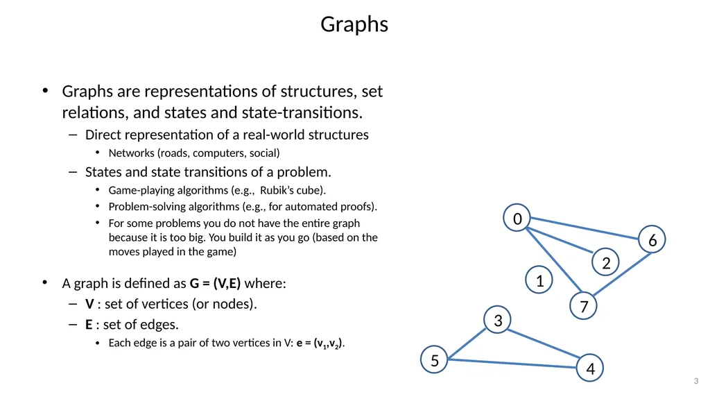
Graphs Graphs are representations of structures, set relations, and states and state-transitions.
Direct representation of a real-world structures
Networks (roads, computers, social)
States and state transitions of a problem.
Game-playing algorithms (e.g., Rubik’s cube).
Problem-solving algorithms (e.g., for automated proofs).
For some problems you do not have the entire graph because it is too big. You build it as you go (based on the moves played in the game)
A graph is defined as G = (V,E) where:
V : set of vertices (or nodes).
E : set of edges.
Each edge is a pair of two vertices in V: e = (v1,v2). 3<br>
Direct representation of a real-world structures
Networks (roads, computers, social)
States and state transitions of a problem.
Game-playing algorithms (e.g., Rubik’s cube).
Problem-solving algorithms (e.g., for automated proofs).
For some problems you do not have the entire graph because it is too big. You build it as you go (based on the moves played in the game)
A graph is defined as G = (V,E) where:
V : set of vertices (or nodes).
E : set of edges.
Each edge is a pair of two vertices in V: e = (v1,v2). 3<br>
04
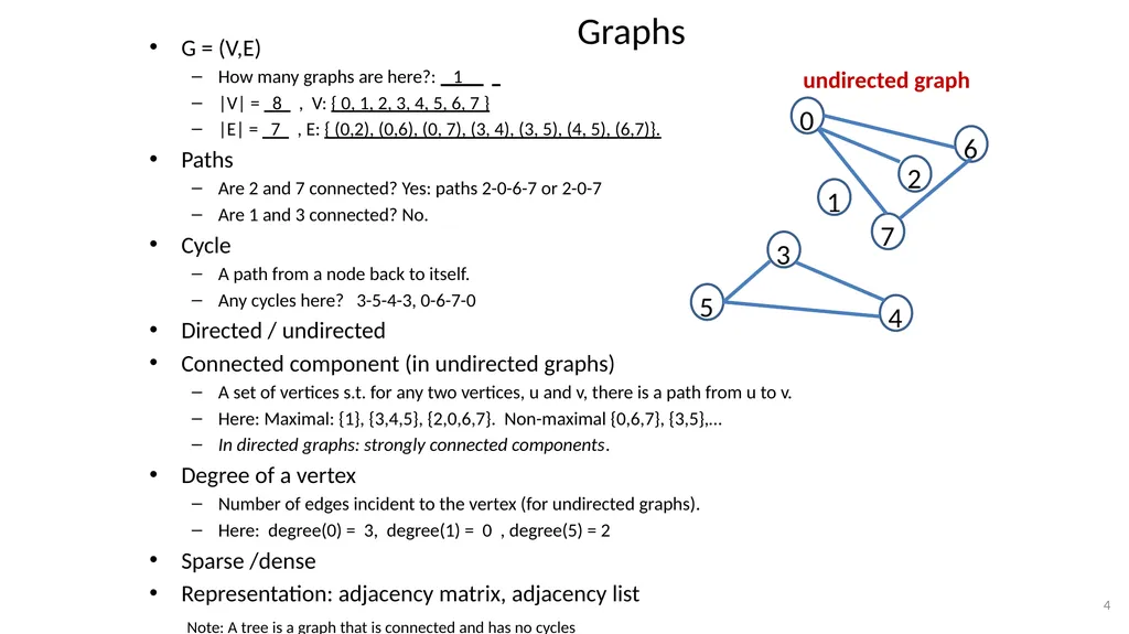
Graphs G = (V,E)
How many graphs are here?: 1
|V| = 8 , V: { 0, 1, 2, 3, 4, 5, 6, 7 }
|E| = 7 , E: { (0,2), (0,6), (0, 7), (3, 4), (3, 5), (4, 5), (6,7)}.
Paths
Are 2 and 7 connected? Yes: paths 2-0-6-7 or 2-0-7
Are 1 and 3 connected? No.
Cycle
A path from a node back to itself.
Any cycles here? 3-5-4-3, 0-6-7-0
Directed / undirected
Connected component (in undirected graphs)
A set of vertices s.t. for any two vertices, u and v, there is a path from u to v.
Here: Maximal: {1}, {3,4,5}, {2,0,6,7}. Non-maximal {0,6,7}, {3,5},…
In directed graphs: strongly connected components.
Degree of a vertex
Number of edges incident to the vertex (for undirected graphs).
Here: degree(0) = 3, degree(1) = 0 , degree(5) = 2
Sparse /dense
Representation: adjacency matrix, adjacency list 4 undirected graph Note: A tree is a graph that is connected and has no cycles<br>
How many graphs are here?: 1
|V| = 8 , V: { 0, 1, 2, 3, 4, 5, 6, 7 }
|E| = 7 , E: { (0,2), (0,6), (0, 7), (3, 4), (3, 5), (4, 5), (6,7)}.
Paths
Are 2 and 7 connected? Yes: paths 2-0-6-7 or 2-0-7
Are 1 and 3 connected? No.
Cycle
A path from a node back to itself.
Any cycles here? 3-5-4-3, 0-6-7-0
Directed / undirected
Connected component (in undirected graphs)
A set of vertices s.t. for any two vertices, u and v, there is a path from u to v.
Here: Maximal: {1}, {3,4,5}, {2,0,6,7}. Non-maximal {0,6,7}, {3,5},…
In directed graphs: strongly connected components.
Degree of a vertex
Number of edges incident to the vertex (for undirected graphs).
Here: degree(0) = 3, degree(1) = 0 , degree(5) = 2
Sparse /dense
Representation: adjacency matrix, adjacency list 4 undirected graph Note: A tree is a graph that is connected and has no cycles<br>
05
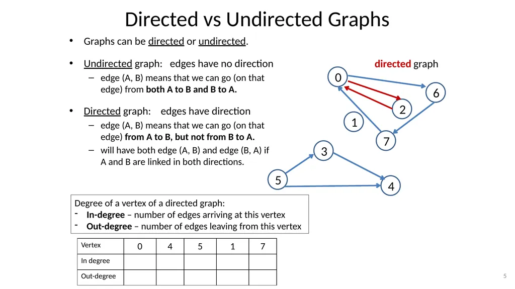
Directed vs Undirected Graphs Graphs can be directed or undirected.
Undirected graph: edges have no direction
edge (A, B) means that we can go (on that edge) from both A to B and B to A.
Directed graph: edges have direction
edge (A, B) means that we can go (on that edge) from A to B, but not from B to A.
will have both edge (A, B) and edge (B, A) if A and B are linked in both directions. 5 directed graph Degree of a vertex of a directed graph:
In-degree – number of edges arriving at this vertex
Out-degree – number of edges leaving from this vertex<br>
Undirected graph: edges have no direction
edge (A, B) means that we can go (on that edge) from both A to B and B to A.
Directed graph: edges have direction
edge (A, B) means that we can go (on that edge) from A to B, but not from B to A.
will have both edge (A, B) and edge (B, A) if A and B are linked in both directions. 5 directed graph Degree of a vertex of a directed graph:
In-degree – number of edges arriving at this vertex
Out-degree – number of edges leaving from this vertex<br>
06
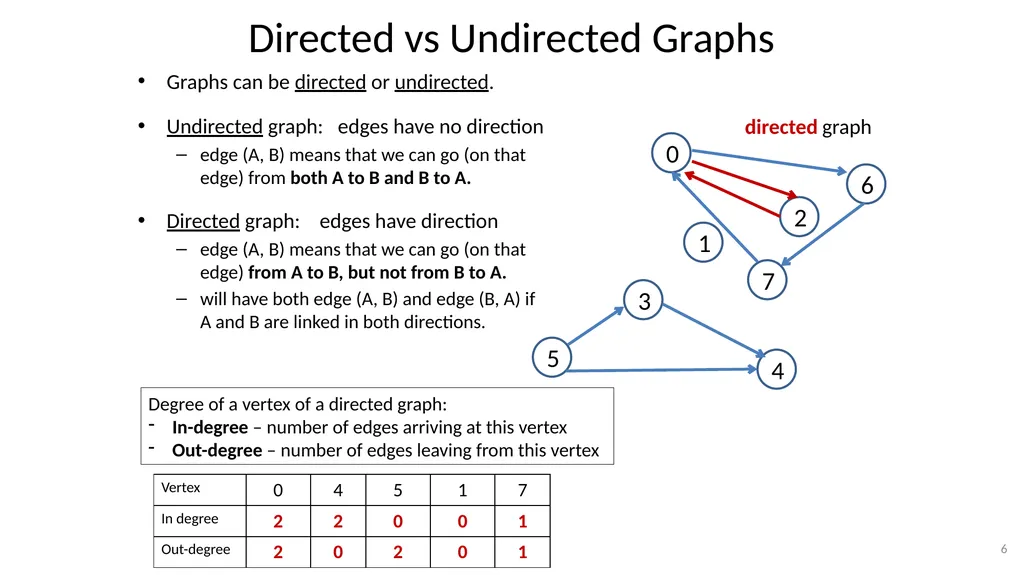
Directed vs Undirected Graphs Graphs can be directed or undirected.
Undirected graph: edges have no direction
edge (A, B) means that we can go (on that edge) from both A to B and B to A.
Directed graph: edges have direction
edge (A, B) means that we can go (on that edge) from A to B, but not from B to A.
will have both edge (A, B) and edge (B, A) if A and B are linked in both directions. 6 Degree of a vertex of a directed graph:
In-degree – number of edges arriving at this vertex
Out-degree – number of edges leaving from this vertex<br>
Undirected graph: edges have no direction
edge (A, B) means that we can go (on that edge) from both A to B and B to A.
Directed graph: edges have direction
edge (A, B) means that we can go (on that edge) from A to B, but not from B to A.
will have both edge (A, B) and edge (B, A) if A and B are linked in both directions. 6 Degree of a vertex of a directed graph:
In-degree – number of edges arriving at this vertex
Out-degree – number of edges leaving from this vertex<br>
07
Strongly Connected Components
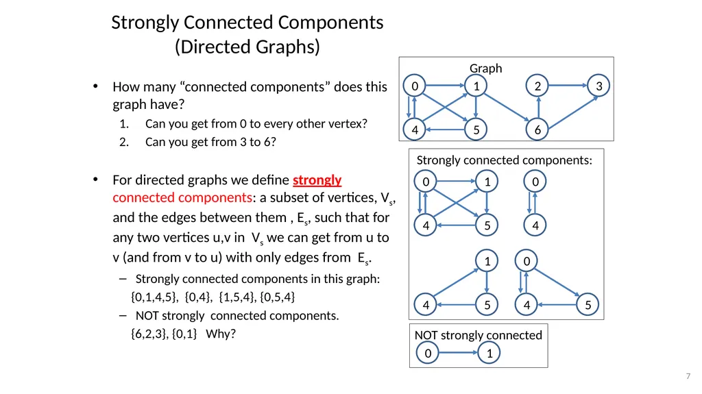
(Directed Graphs) How many “connected components” does this graph have?
Can you get from 0 to every other vertex?
Can you get from 3 to 6?
For directed graphs we define strongly connected components: a subset of vertices, Vs, and the edges between them , Es, such that for any two vertices u,v in Vs we can get from u to v (and from v to u) with only edges from Es.
Strongly connected components in this graph:
{0,1,4,5}, {0,4}, {1,5,4}, {0,5,4}
NOT strongly connected components.
{6,2,3}, {0,1} Why? 7 0 1 4 5 6 2 3 0 1 4 5 1 4 5 0 4 5 0 4 Strongly connected components: 0 1 NOT strongly connected Graph<br>
Can you get from 0 to every other vertex?
Can you get from 3 to 6?
For directed graphs we define strongly connected components: a subset of vertices, Vs, and the edges between them , Es, such that for any two vertices u,v in Vs we can get from u to v (and from v to u) with only edges from Es.
Strongly connected components in this graph:
{0,1,4,5}, {0,4}, {1,5,4}, {0,5,4}
NOT strongly connected components.
{6,2,3}, {0,1} Why? 7 0 1 4 5 6 2 3 0 1 4 5 1 4 5 0 4 5 0 4 Strongly connected components: 0 1 NOT strongly connected Graph<br>
08
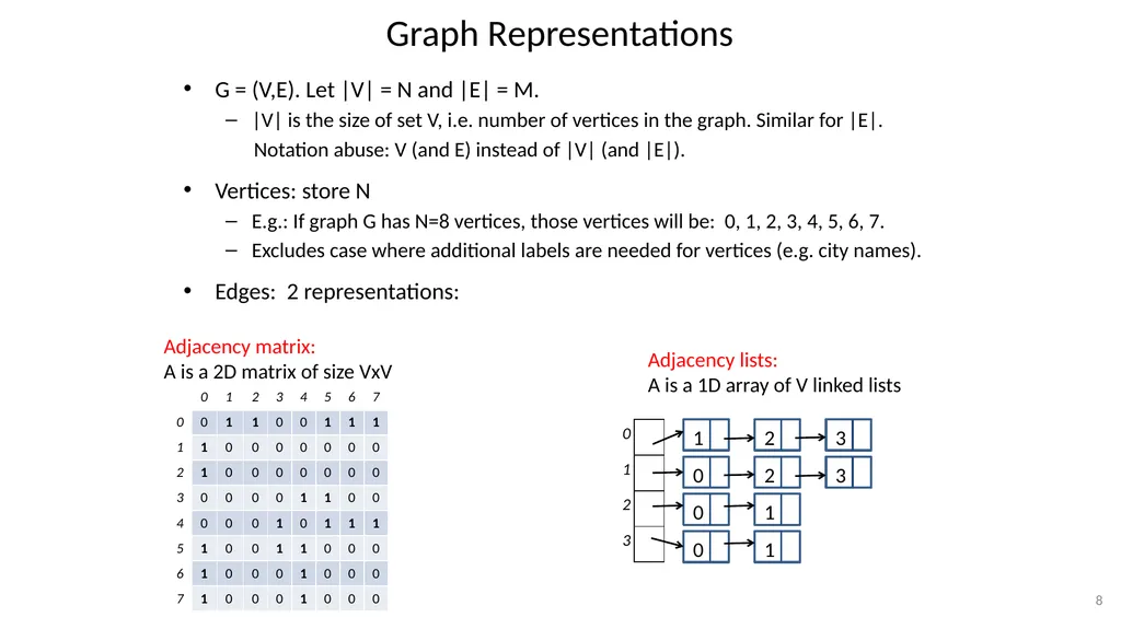
Graph Representations G = (V,E). Let |V| = N and |E| = M.
|V| is the size of set V, i.e. number of vertices in the graph. Similar for |E|.
Notation abuse: V (and E) instead of |V| (and |E|).
Vertices: store N
E.g.: If graph G has N=8 vertices, those vertices will be: 0, 1, 2, 3, 4, 5, 6, 7.
Excludes case where additional labels are needed for vertices (e.g. city names).
Edges: 2 representations: 8 Adjacency matrix:
A is a 2D matrix of size VxV Adjacency lists:
A is a 1D array of V linked lists<br>
|V| is the size of set V, i.e. number of vertices in the graph. Similar for |E|.
Notation abuse: V (and E) instead of |V| (and |E|).
Vertices: store N
E.g.: If graph G has N=8 vertices, those vertices will be: 0, 1, 2, 3, 4, 5, 6, 7.
Excludes case where additional labels are needed for vertices (e.g. city names).
Edges: 2 representations: 8 Adjacency matrix:
A is a 2D matrix of size VxV Adjacency lists:
A is a 1D array of V linked lists<br>
09
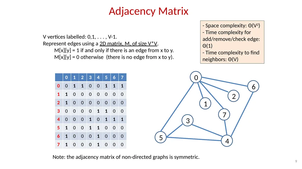
Adjacency Matrix 9 V vertices labelled: 0,1, . . . , V-1.
Represent edges using a 2D matrix, M, of size V*V.
M[x][y] = 1 if and only if there is an edge from x to y.
M[x][y] = 0 otherwise (there is no edge from x to y). - Space complexity: Θ(V2)
- Time complexity for add/remove/check edge: Θ(1)
- Time complexity to find neighbors: Θ(V) Note: the adjacency matrix of non-directed graphs is symmetric.<br>
Represent edges using a 2D matrix, M, of size V*V.
M[x][y] = 1 if and only if there is an edge from x to y.
M[x][y] = 0 otherwise (there is no edge from x to y). - Space complexity: Θ(V2)
- Time complexity for add/remove/check edge: Θ(1)
- Time complexity to find neighbors: Θ(V) Note: the adjacency matrix of non-directed graphs is symmetric.<br>
10
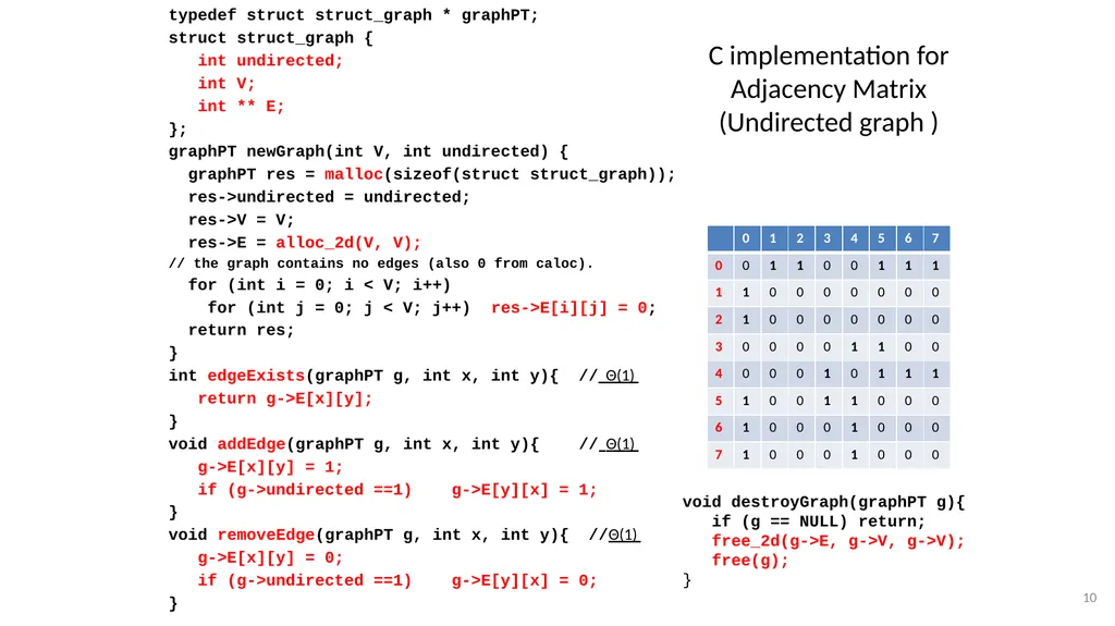
C implementation for Adjacency Matrix (Undirected graph ) typedef struct struct_graph * graphPT;
struct struct_graph {
int undirected;
int V;
int ** E;
};
graphPT newGraph(int V, int undirected) {
graphPT res = malloc(sizeof(struct struct_graph));
res->undirected = undirected;
res->V = V;
res->E = alloc_2d(V, V);
// the graph contains no edges (also 0 from caloc).
for (int i = 0; i < V; i++)
for (int j = 0; j < V; j++) res->E[i][j] = 0;
return res;
}
int edgeExists(graphPT g, int x, int y){ // Θ(1)
return g->E[x][y];
}
void addEdge(graphPT g, int x, int y){ // Θ(1)
g->E[x][y] = 1;
if (g->undirected ==1) g->E[y][x] = 1;
}
void removeEdge(graphPT g, int x, int y){ //Θ(1)
g->E[x][y] = 0;
if (g->undirected ==1) g->E[y][x] = 0;
} 10 void destroyGraph(graphPT g){
if (g == NULL) return;
free_2d(g->E, g->V, g->V);
free(g);
}<br>
struct struct_graph {
int undirected;
int V;
int ** E;
};
graphPT newGraph(int V, int undirected) {
graphPT res = malloc(sizeof(struct struct_graph));
res->undirected = undirected;
res->V = V;
res->E = alloc_2d(V, V);
// the graph contains no edges (also 0 from caloc).
for (int i = 0; i < V; i++)
for (int j = 0; j < V; j++) res->E[i][j] = 0;
return res;
}
int edgeExists(graphPT g, int x, int y){ // Θ(1)
return g->E[x][y];
}
void addEdge(graphPT g, int x, int y){ // Θ(1)
g->E[x][y] = 1;
if (g->undirected ==1) g->E[y][x] = 1;
}
void removeEdge(graphPT g, int x, int y){ //Θ(1)
g->E[x][y] = 0;
if (g->undirected ==1) g->E[y][x] = 0;
} 10 void destroyGraph(graphPT g){
if (g == NULL) return;
free_2d(g->E, g->V, g->V);
free(g);
}<br>
11
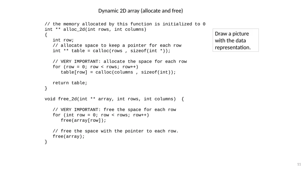
11 // the memory allocated by this function is initialized to 0
int ** alloc_2d(int rows, int columns)
{
int row;
// allocate space to keep a pointer for each row
int ** table = calloc(rows , sizeof(int *));
// VERY IMPORTANT: allocate the space for each row
for (row = 0; row < rows; row++)
table[row] = calloc(columns , sizeof(int));
return table;
}
void free_2d(int ** array, int rows, int columns) {
// VERY IMPORTANT: free the space for each row
for (int row = 0; row < rows; row++)
free(array[row]);
// free the space with the pointer to each row.
free(array);
} Dynamic 2D array (allocate and free) Draw a picture with the data representation.<br>
int ** alloc_2d(int rows, int columns)
{
int row;
// allocate space to keep a pointer for each row
int ** table = calloc(rows , sizeof(int *));
// VERY IMPORTANT: allocate the space for each row
for (row = 0; row < rows; row++)
table[row] = calloc(columns , sizeof(int));
return table;
}
void free_2d(int ** array, int rows, int columns) {
// VERY IMPORTANT: free the space for each row
for (int row = 0; row < rows; row++)
free(array[row]);
// free the space with the pointer to each row.
free(array);
} Dynamic 2D array (allocate and free) Draw a picture with the data representation.<br>
12
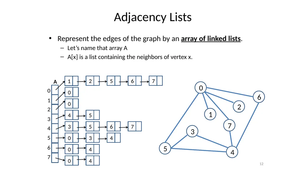
Adjacency Lists 12 1 0 3 2 5 7 4 6 A Represent the edges of the graph by an array of linked lists.
Let’s name that array A
A[x] is a list containing the neighbors of vertex x.<br>
Let’s name that array A
A[x] is a list containing the neighbors of vertex x.<br>
13
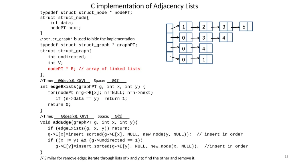
C implementation of Adjacency Lists typedef struct struct_node * nodePT;
struct struct_node{
int data;
nodePT next;
}
// struct_graph* is used to hide the implementation
typedef struct struct_graph * graphPT;
struct struct_graph{
int undirected;
int V;
nodePT * E; // array of linked lists
};
//Time: Θ(deg(x)), O(V) Space: Θ(1) _
int edgeExists(graphPT g, int x, int y) {
for(nodePt n=g->E[x]; n!=NULL; n=n->next)
if (n->data == y) return 1;
return 0;
}
//Time: Θ(deg(x)), O(V) Space: Θ(1) _
void addEdge(graphPT g, int x, int y){
if (edgeExists(g, x, y)) return;
g->E[x]=insert_sorted(g->E[x], NULL, new_node(y, NULL)); // insert in order
if ((x != y) && (g->undirected == 1))
g->E[y]=insert_sorted(g->E[y], NULL, new_node(x, NULL)); //insert in order
}
// Similar for remove edge: iterate through lists of x and y to find the other and remove it. 13<br>
struct struct_node{
int data;
nodePT next;
}
// struct_graph* is used to hide the implementation
typedef struct struct_graph * graphPT;
struct struct_graph{
int undirected;
int V;
nodePT * E; // array of linked lists
};
//Time: Θ(deg(x)), O(V) Space: Θ(1) _
int edgeExists(graphPT g, int x, int y) {
for(nodePt n=g->E[x]; n!=NULL; n=n->next)
if (n->data == y) return 1;
return 0;
}
//Time: Θ(deg(x)), O(V) Space: Θ(1) _
void addEdge(graphPT g, int x, int y){
if (edgeExists(g, x, y)) return;
g->E[x]=insert_sorted(g->E[x], NULL, new_node(y, NULL)); // insert in order
if ((x != y) && (g->undirected == 1))
g->E[y]=insert_sorted(g->E[y], NULL, new_node(x, NULL)); //insert in order
}
// Similar for remove edge: iterate through lists of x and y to find the other and remove it. 13<br>
14
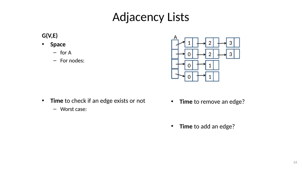
Adjacency Lists G(V,E)
Space
for A
For nodes:
Time to check if an edge exists or not
Worst case: 14 Time to remove an edge?
Time to add an edge? A<br>
Space
for A
For nodes:
Time to check if an edge exists or not
Worst case: 14 Time to remove an edge?
Time to add an edge? A<br>
15
Adjacency Lists G(V,E)
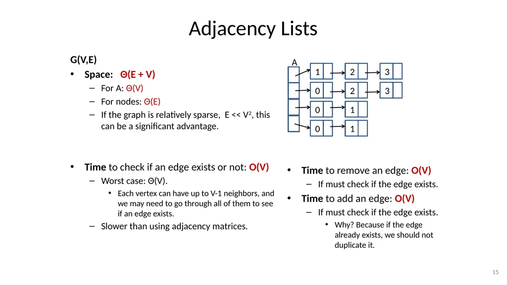
Space: Θ(E + V)
For A: Θ(V)
For nodes: Θ(E)
If the graph is relatively sparse, E << V2, this can be a significant advantage.
Time to check if an edge exists or not: O(V)
Worst case: Θ(V).
Each vertex can have up to V-1 neighbors, and we may need to go through all of them to see if an edge exists.
Slower than using adjacency matrices. 15 Time to remove an edge: O(V)
If must check if the edge exists.
Time to add an edge: O(V)
If must check if the edge exists.
Why? Because if the edge already exists, we should not duplicate it. A<br>
Space: Θ(E + V)
For A: Θ(V)
For nodes: Θ(E)
If the graph is relatively sparse, E << V2, this can be a significant advantage.
Time to check if an edge exists or not: O(V)
Worst case: Θ(V).
Each vertex can have up to V-1 neighbors, and we may need to go through all of them to see if an edge exists.
Slower than using adjacency matrices. 15 Time to remove an edge: O(V)
If must check if the edge exists.
Time to add an edge: O(V)
If must check if the edge exists.
Why? Because if the edge already exists, we should not duplicate it. A<br>
16
Check Out Posted Code graph.h: defines an abstract interface for basic graph functions.
graph_matrix.c: implements the abstract interface of graph.h, using an adjacency matrix. See also: twoD_arrays.h, twoD_arrays.c for a 2D matrix implemention.
graph_list.c: also implements the abstract interface of graph.h, using adjacency lists.
graph_main: a test program, that can be compiled with either graph_matrix.c or graphs_list.c. 16<br>
graph_matrix.c: implements the abstract interface of graph.h, using an adjacency matrix. See also: twoD_arrays.h, twoD_arrays.c for a 2D matrix implemention.
graph_list.c: also implements the abstract interface of graph.h, using adjacency lists.
graph_main: a test program, that can be compiled with either graph_matrix.c or graphs_list.c. 16<br>
17
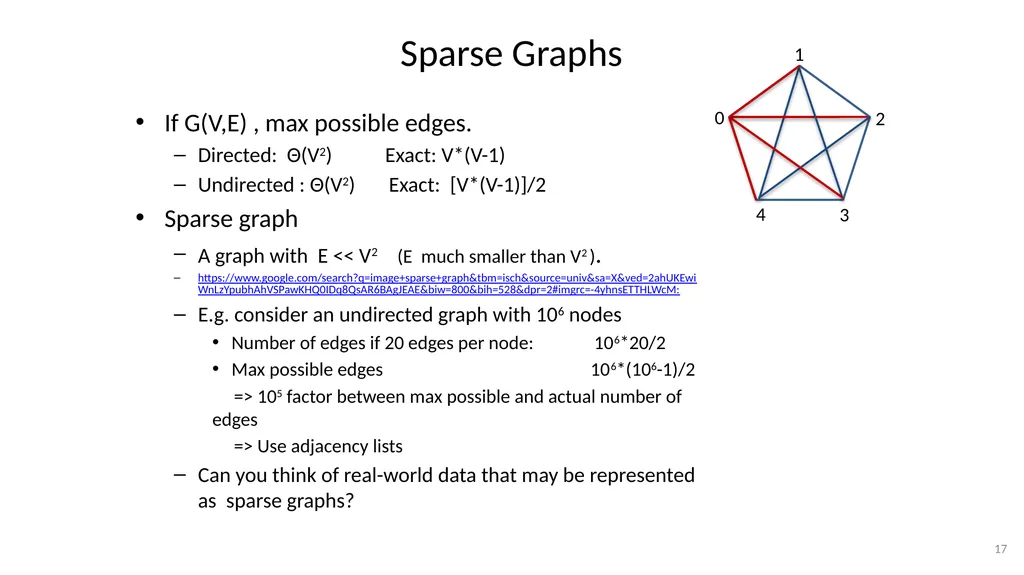
Sparse Graphs If G(V,E) , max possible edges.
Directed: Θ(V2) Exact: V*(V-1)
Undirected : Θ(V2) Exact: [V*(V-1)]/2
Sparse graph
A graph with E << V2 (E much smaller than V2 ).
https://www.google.com/search?q=image+sparse+graph&tbm=isch&source=univ&sa=X&ved=2ahUKEwiWnLzYpubhAhVSPawKHQ0IDq8QsAR6BAgJEAE&biw=800&bih=528&dpr=2#imgrc=-4yhnsETTHLWcM:
E.g. consider an undirected graph with 106 nodes
Number of edges if 20 edges per node: 106*20/2
Max possible edges 106*(106-1)/2
=> 105 factor between max possible and actual number of edges
=> Use adjacency lists
Can you think of real-world data that may be represented as sparse graphs? 17<br>
Directed: Θ(V2) Exact: V*(V-1)
Undirected : Θ(V2) Exact: [V*(V-1)]/2
Sparse graph
A graph with E << V2 (E much smaller than V2 ).
https://www.google.com/search?q=image+sparse+graph&tbm=isch&source=univ&sa=X&ved=2ahUKEwiWnLzYpubhAhVSPawKHQ0IDq8QsAR6BAgJEAE&biw=800&bih=528&dpr=2#imgrc=-4yhnsETTHLWcM:
E.g. consider an undirected graph with 106 nodes
Number of edges if 20 edges per node: 106*20/2
Max possible edges 106*(106-1)/2
=> 105 factor between max possible and actual number of edges
=> Use adjacency lists
Can you think of real-world data that may be represented as sparse graphs? 17<br>
18
Student self study: Space Analysis:
Adjacency Matrices vs. Adjacency Lists Suppose we have an undirected graph with:
10 million vertices.
Each vertex has at most 20 neighbors.
Individual practice: Calculate the minimum space needed to store this graph in each representation. Use/assume:
A matrix of BITS for the matrix representation
An int is stored on 8 bytes and a memory address is stored on 8 bytes as well.
Calculate the space requirement (actual number, not Θ) for each representation.
Compare your result with the numbers below.
Check your solution against the posted one. Clarify next lecture any questions you may have.
Adjacency matrices: we need at least 100 trillion bits of memory, so at least 12.5TB of memory.
Adjacency lists: in total, they would store at most 200 million nodes. With 16 bytes per node (as an example), this takes at most 3.28 Gigabytes.
We’ll see next how to compute/verify such answers. 18<br>
10 million vertices.
Each vertex has at most 20 neighbors.
Individual practice: Calculate the minimum space needed to store this graph in each representation. Use/assume:
A matrix of BITS for the matrix representation
An int is stored on 8 bytes and a memory address is stored on 8 bytes as well.
Calculate the space requirement (actual number, not Θ) for each representation.
Compare your result with the numbers below.
Check your solution against the posted one. Clarify next lecture any questions you may have.
Adjacency matrices: we need at least 100 trillion bits of memory, so at least 12.5TB of memory.
Adjacency lists: in total, they would store at most 200 million nodes. With 16 bytes per node (as an example), this takes at most 3.28 Gigabytes.
We’ll see next how to compute/verify such answers. 18<br>
19
Steps for Solving This Problem:
understand all terms and numbers Suppose we have an undirected graph with:
10 million vertices.
Each vertex has at most 20 neighbors.
Adjacency matrices: we need at least 100 trillion bits of memory, so at least 12.5TB of memory.
Adjacency lists: in total, they would store at most 100 million nodes. With 16 bytes per node (as an example), this takes 3.28 Gigabytes.
Find ‘keywords’, understand numbers:
10 million vertices => 10 * 106
Trillion = 1012
1 TB (terra bytes) = 1012 bytes
1GB = 109 bytes
100 Trillion bits vs 12.5 TB (terra bytes) 19<br>
10 million vertices.
Each vertex has at most 20 neighbors.
Adjacency matrices: we need at least 100 trillion bits of memory, so at least 12.5TB of memory.
Adjacency lists: in total, they would store at most 100 million nodes. With 16 bytes per node (as an example), this takes 3.28 Gigabytes.
Find ‘keywords’, understand numbers:
10 million vertices => 10 * 106
Trillion = 1012
1 TB (terra bytes) = 1012 bytes
1GB = 109 bytes
100 Trillion bits vs 12.5 TB (terra bytes) 19<br>
20
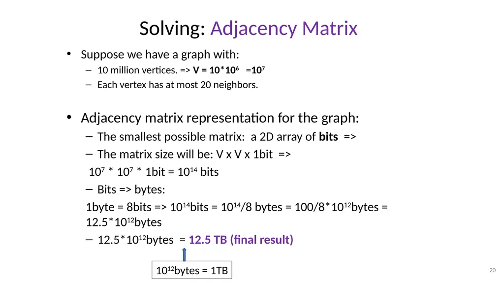
Solving: Adjacency Matrix Suppose we have a graph with:
10 million vertices. => V = 10*106 =107
Each vertex has at most 20 neighbors.
Adjacency matrix representation for the graph:
The smallest possible matrix: a 2D array of bits =>
The matrix size will be: V x V x 1bit =>
107 * 107 * 1bit = 1014 bits
Bits => bytes:
1byte = 8bits => 1014bits = 1014/8 bytes = 100/8*1012bytes = 12.5*1012bytes
12.5*1012bytes = 12.5 TB (final result) 20 1012bytes = 1TB<br>
10 million vertices. => V = 10*106 =107
Each vertex has at most 20 neighbors.
Adjacency matrix representation for the graph:
The smallest possible matrix: a 2D array of bits =>
The matrix size will be: V x V x 1bit =>
107 * 107 * 1bit = 1014 bits
Bits => bytes:
1byte = 8bits => 1014bits = 1014/8 bytes = 100/8*1012bytes = 12.5*1012bytes
12.5*1012bytes = 12.5 TB (final result) 20 1012bytes = 1TB<br>
21
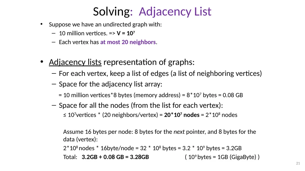
Solving: Adjacency List Suppose we have an undirected graph with:
10 million vertices. => V = 107
Each vertex has at most 20 neighbors.
Adjacency lists representation of graphs:
For each vertex, keep a list of edges (a list of neighboring vertices)
Space for the adjacency list array:
= 10 million vertices*8 bytes (memory address) = 8*107 bytes = 0.08 GB
Space for all the nodes (from the list for each vertex):
≤ 107vertices * (20 neighbors/vertex) = 20*107 nodes = 2*108 nodes
Assume 16 bytes per node: 8 bytes for the next pointer, and 8 bytes for the data (vertex):
2*108 nodes * 16byte/node = 32 * 108 bytes = 3.2 * 109 bytes = 3.2GB
Total: 3.2GB + 0.08 GB = 3.28GB ( 109 bytes = 1GB (GigaByte) ) 21<br>
10 million vertices. => V = 107
Each vertex has at most 20 neighbors.
Adjacency lists representation of graphs:
For each vertex, keep a list of edges (a list of neighboring vertices)
Space for the adjacency list array:
= 10 million vertices*8 bytes (memory address) = 8*107 bytes = 0.08 GB
Space for all the nodes (from the list for each vertex):
≤ 107vertices * (20 neighbors/vertex) = 20*107 nodes = 2*108 nodes
Assume 16 bytes per node: 8 bytes for the next pointer, and 8 bytes for the data (vertex):
2*108 nodes * 16byte/node = 32 * 108 bytes = 3.2 * 109 bytes = 3.2GB
Total: 3.2GB + 0.08 GB = 3.28GB ( 109 bytes = 1GB (GigaByte) ) 21<br>
22
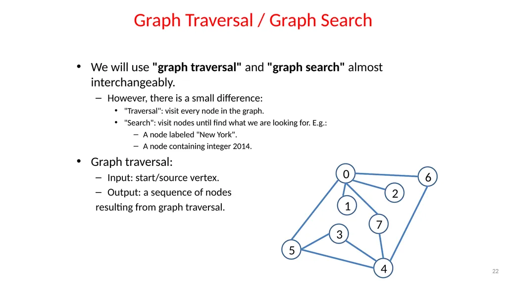
Graph Traversal / Graph Search We will use "graph traversal" and "graph search" almost interchangeably.
However, there is a small difference:
"Traversal": visit every node in the graph.
"Search": visit nodes until find what we are looking for. E.g.:
A node labeled "New York".
A node containing integer 2014.
Graph traversal:
Input: start/source vertex.
Output: a sequence of nodes
resulting from graph traversal. 22<br>
However, there is a small difference:
"Traversal": visit every node in the graph.
"Search": visit nodes until find what we are looking for. E.g.:
A node labeled "New York".
A node containing integer 2014.
Graph traversal:
Input: start/source vertex.
Output: a sequence of nodes
resulting from graph traversal. 22<br>
23
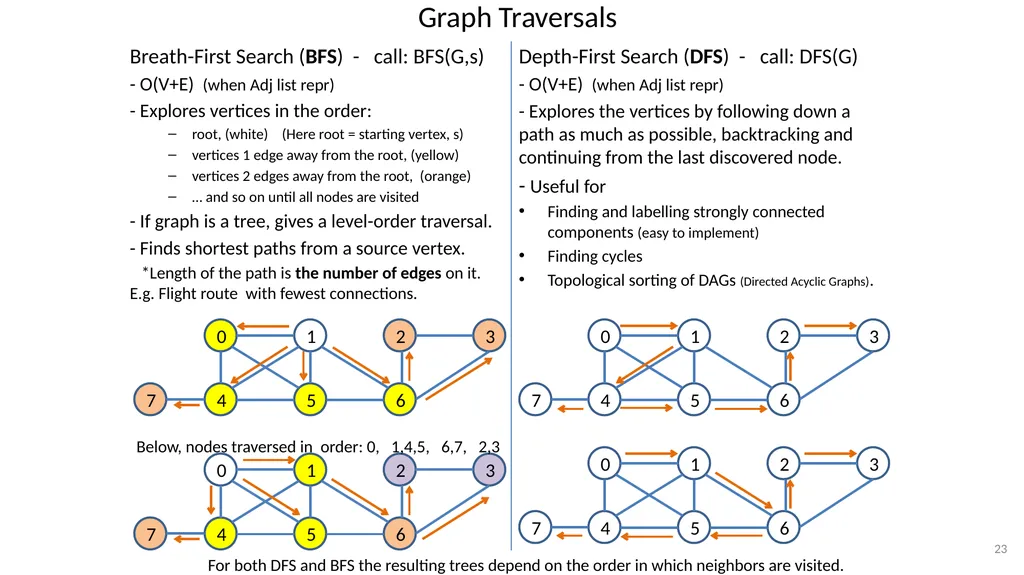
Depth-First Search (DFS) - call: DFS(G)
- O(V+E) (when Adj list repr)
- Explores the vertices by following down a path as much as possible, backtracking and continuing from the last discovered node.
- Useful for
Finding and labelling strongly connected components (easy to implement)
Finding cycles
Topological sorting of DAGs (Directed Acyclic Graphs). 23 Breath-First Search (BFS) - call: BFS(G,s)
- O(V+E) (when Adj list repr)
- Explores vertices in the order:
root, (white) (Here root = starting vertex, s)
vertices 1 edge away from the root, (yellow)
vertices 2 edges away from the root, (orange)
… and so on until all nodes are visited
- If graph is a tree, gives a level-order traversal.
- Finds shortest paths from a source vertex.
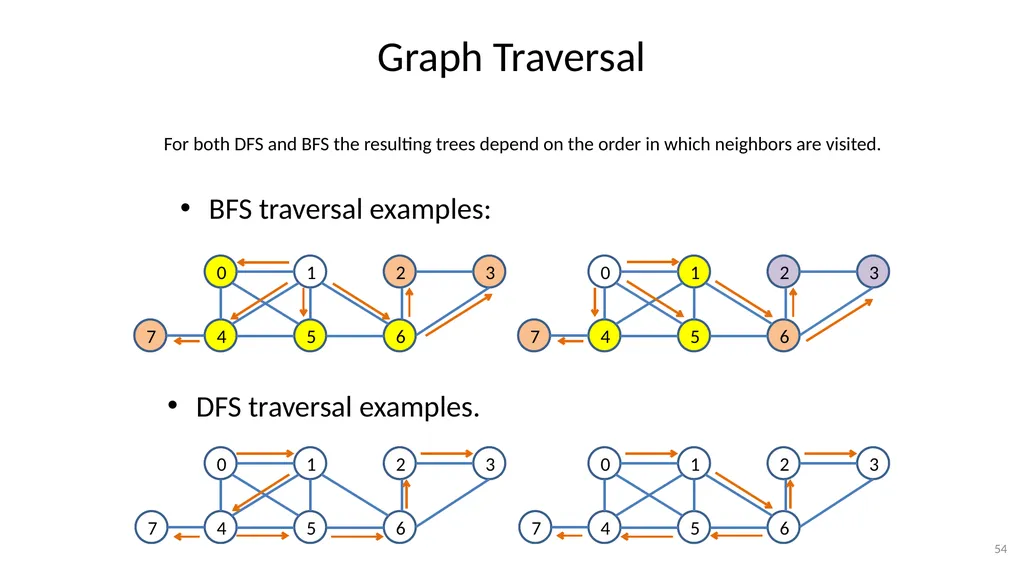
*Length of the path is the number of edges on it. E.g. Flight route with fewest connections. For both DFS and BFS the resulting trees depend on the order in which neighbors are visited. Graph Traversals Below, nodes traversed in order: 0, 1,4,5, 6,7, 2,3<br>
- O(V+E) (when Adj list repr)
- Explores the vertices by following down a path as much as possible, backtracking and continuing from the last discovered node.
- Useful for
Finding and labelling strongly connected components (easy to implement)
Finding cycles
Topological sorting of DAGs (Directed Acyclic Graphs). 23 Breath-First Search (BFS) - call: BFS(G,s)
- O(V+E) (when Adj list repr)
- Explores vertices in the order:
root, (white) (Here root = starting vertex, s)
vertices 1 edge away from the root, (yellow)
vertices 2 edges away from the root, (orange)
… and so on until all nodes are visited
- If graph is a tree, gives a level-order traversal.
- Finds shortest paths from a source vertex.
*Length of the path is the number of edges on it. E.g. Flight route with fewest connections. For both DFS and BFS the resulting trees depend on the order in which neighbors are visited. Graph Traversals Below, nodes traversed in order: 0, 1,4,5, 6,7, 2,3<br>
24
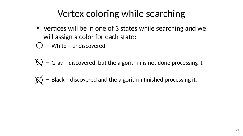
Vertex coloring while searching Vertices will be in one of 3 states while searching and we will assign a color for each state:
White – undiscovered
Gray – discovered, but the algorithm is not done processing it
Black – discovered and the algorithm finished processing it. 24<br>
White – undiscovered
Gray – discovered, but the algorithm is not done processing it
Black – discovered and the algorithm finished processing it. 24<br>
25
Breadth-First Search (BFS)
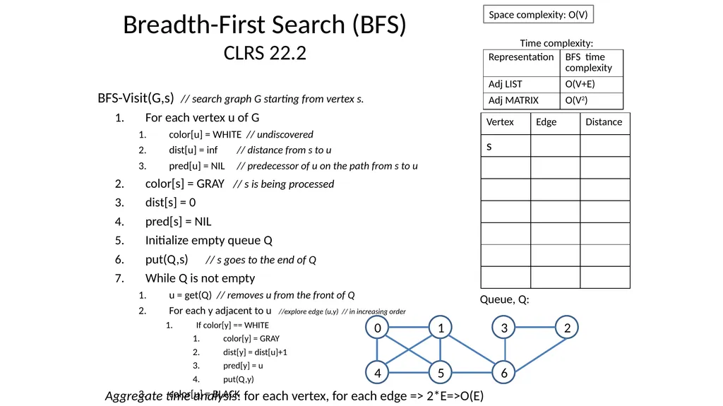
CLRS 22.2 BFS-Visit(G,s) // search graph G starting from vertex s.
For each vertex u of G
color[u] = WHITE // undiscovered
dist[u] = inf // distance from s to u
pred[u] = NIL // predecessor of u on the path from s to u
color[s] = GRAY // s is being processed
dist[s] = 0
pred[s] = NIL
Initialize empty queue Q
put(Q,s) // s goes to the end of Q
While Q is not empty
u = get(Q) // removes u from the front of Q
For each y adjacent to u //explore edge (u,y) // in increasing order
If color[y] == WHITE
color[y] = GRAY
dist[y] = dist[u]+1
pred[y] = u
put(Q,y)
color[u] = BLACK 25 Aggregate time analysis: for each vertex, for each edge => 2*E=>O(E) Queue, Q: Space complexity: O(V) Time complexity:<br>
For each vertex u of G
color[u] = WHITE // undiscovered
dist[u] = inf // distance from s to u
pred[u] = NIL // predecessor of u on the path from s to u
color[s] = GRAY // s is being processed
dist[s] = 0
pred[s] = NIL
Initialize empty queue Q
put(Q,s) // s goes to the end of Q
While Q is not empty
u = get(Q) // removes u from the front of Q
For each y adjacent to u //explore edge (u,y) // in increasing order
If color[y] == WHITE
color[y] = GRAY
dist[y] = dist[u]+1
pred[y] = u
put(Q,y)
color[u] = BLACK 25 Aggregate time analysis: for each vertex, for each edge => 2*E=>O(E) Queue, Q: Space complexity: O(V) Time complexity:<br>
26
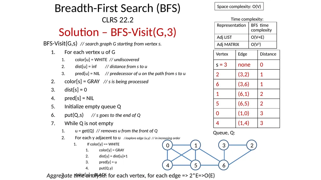
Breadth-First Search (BFS)
CLRS 22.2
Solution – BFS-Visit(G,3) BFS-Visit(G,s) // search graph G starting from vertex s.
For each vertex u of G
color[u] = WHITE // undiscovered
dist[u] = inf // distance from s to u
pred[u] = NIL // predecessor of u on the path from s to u
color[s] = GRAY // s is being processed
dist[s] = 0
pred[s] = NIL
Initialize empty queue Q
put(Q,s) // s goes to the end of Q
While Q is not empty
u = get(Q) // removes u from the front of Q
For each y adjacent to u //explore edge (u,y) // in increasing order
If color[y] == WHITE
color[y] = GRAY
dist[y] = dist[u]+1
pred[y] = u
put(Q,y)
color[u] = BLACK 26 Aggregate time analysis: for each vertex, for each edge => 2*E=>O(E) Queue, Q: Space complexity: O(V) Time complexity:<br>
For each vertex u of G
color[u] = WHITE // undiscovered
dist[u] = inf // distance from s to u
pred[u] = NIL // predecessor of u on the path from s to u
color[s] = GRAY // s is being processed
dist[s] = 0
pred[s] = NIL
Initialize empty queue Q
put(Q,s) // s goes to the end of Q
While Q is not empty
u = get(Q) // removes u from the front of Q
For each y adjacent to u //explore edge (u,y) // in increasing order
If color[y] == WHITE
color[y] = GRAY
dist[y] = dist[u]+1
pred[y] = u
put(Q,y)
color[u] = BLACK 26 Aggregate time analysis: for each vertex, for each edge => 2*E=>O(E) Queue, Q: Space complexity: O(V) Time complexity:<br>
27
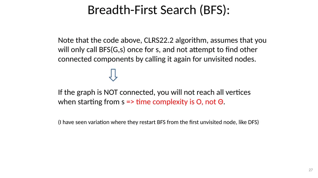
Breadth-First Search (BFS): Note that the code above, CLRS22.2 algorithm, assumes that you will only call BFS(G,s) once for s, and not attempt to find other connected components by calling it again for unvisited nodes.
If the graph is NOT connected, you will not reach all vertices when starting from s => time complexity is O, not Θ.
(I have seen variation where they restart BFS from the first unvisited node, like DFS) 27<br>
If the graph is NOT connected, you will not reach all vertices when starting from s => time complexity is O, not Θ.
(I have seen variation where they restart BFS from the first unvisited node, like DFS) 27<br>
28
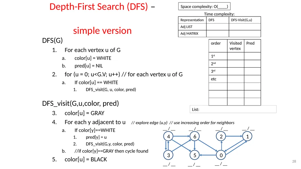
Depth-First Search (DFS) –
simple version DFS(G)
For each vertex u of G
color[u] = WHITE
pred[u] = NIL
for (u = 0; u<G.V; u++) // for each vertex u of G
If color[u] == WHITE
DFS_visit(G, u, color, pred)
DFS_visit(G,u,color, pred)
color[u] = GRAY
For each y adjacent to u // explore edge (u,y) // use increasing order for neighbors
If color[y]==WHITE
pred[y] = u
DFS_visit(G,y, color, pred)
//if color[y]==GRAY then cycle found
color[u] = BLACK 28 4 6 3 5 0 2 1 List: __ / __ __ / __ __ / __ __ / __ __ / __ __ / __ __ / __ Space complexity: O(____) Time complexity:<br>
For each vertex u of G
color[u] = WHITE
pred[u] = NIL
for (u = 0; u<G.V; u++) // for each vertex u of G
If color[u] == WHITE
DFS_visit(G, u, color, pred)
DFS_visit(G,u,color, pred)
color[u] = GRAY
For each y adjacent to u // explore edge (u,y) // use increasing order for neighbors
If color[y]==WHITE
pred[y] = u
DFS_visit(G,y, color, pred)
//if color[y]==GRAY then cycle found
color[u] = BLACK 28 4 6 3 5 0 2 1 List: __ / __ __ / __ __ / __ __ / __ __ / __ __ / __ __ / __ Space complexity: O(____) Time complexity:<br>
29
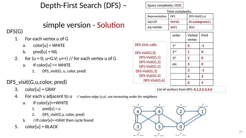
Depth-First Search (DFS) –
simple version - Solution DFS(G)
For each vertex u of G
color[u] = WHITE
pred[u] = NIL
for (u = 0; u<G.V; u++) // for each vertex u of G
If color[u] == WHITE
DFS_visit(G, u, color, pred)
DFS_visit(G,u,color, pred)
color[u] = GRAY
For each y adjacent to u // explore edge (u,y) use increasing order for neighbors
If color[y]==WHITE
pred[y] = u
DFS_visit(G,y, color, pred)
//if color[y]==GRAY then cycle found
color[u] = BLACK 29 4 6 3 5 0 2 1 List of vertices from DFS: 0,1,2,5,3,4,6 __ / __ __ / __ __ / __ __ / __ __ / __ __ / __ __ / __ Space complexity: O(V) Time complexity: DFS-Visit calls:
DFS-visit(G,0)
DFS-Visit(G,1)
DFS-Visit(G,2)
DFS-Visit(G,5)
DFS-Visit(G,3)
DFS-Visit(G,4)
DFS-Visit(G,6)<br>
For each vertex u of G
color[u] = WHITE
pred[u] = NIL
for (u = 0; u<G.V; u++) // for each vertex u of G
If color[u] == WHITE
DFS_visit(G, u, color, pred)
DFS_visit(G,u,color, pred)
color[u] = GRAY
For each y adjacent to u // explore edge (u,y) use increasing order for neighbors
If color[y]==WHITE
pred[y] = u
DFS_visit(G,y, color, pred)
//if color[y]==GRAY then cycle found
color[u] = BLACK 29 4 6 3 5 0 2 1 List of vertices from DFS: 0,1,2,5,3,4,6 __ / __ __ / __ __ / __ __ / __ __ / __ __ / __ __ / __ Space complexity: O(V) Time complexity: DFS-Visit calls:
DFS-visit(G,0)
DFS-Visit(G,1)
DFS-Visit(G,2)
DFS-Visit(G,5)
DFS-Visit(G,3)
DFS-Visit(G,4)
DFS-Visit(G,6)<br>
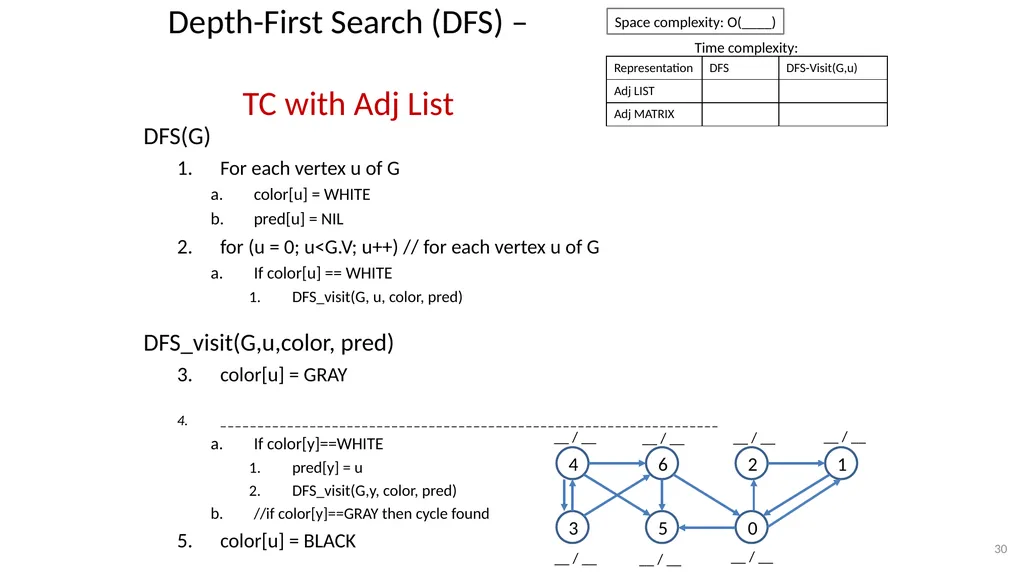
30
Depth-First Search (DFS) –
TC with Adj List DFS(G)
For each vertex u of G
color[u] = WHITE
pred[u] = NIL
for (u = 0; u<G.V; u++) // for each vertex u of G
If color[u] == WHITE
DFS_visit(G, u, color, pred)
DFS_visit(G,u,color, pred)
color[u] = GRAY
___________________________________________________________________
If color[y]==WHITE
pred[y] = u
DFS_visit(G,y, color, pred)
//if color[y]==GRAY then cycle found
color[u] = BLACK 30 4 6 3 5 0 2 1 __ / __ __ / __ __ / __ __ / __ __ / __ __ / __ __ / __ Space complexity: O(____) Time complexity:<br>
For each vertex u of G
color[u] = WHITE
pred[u] = NIL
for (u = 0; u<G.V; u++) // for each vertex u of G
If color[u] == WHITE
DFS_visit(G, u, color, pred)
DFS_visit(G,u,color, pred)
color[u] = GRAY
___________________________________________________________________
If color[y]==WHITE
pred[y] = u
DFS_visit(G,y, color, pred)
//if color[y]==GRAY then cycle found
color[u] = BLACK 30 4 6 3 5 0 2 1 __ / __ __ / __ __ / __ __ / __ __ / __ __ / __ __ / __ Space complexity: O(____) Time complexity:<br>
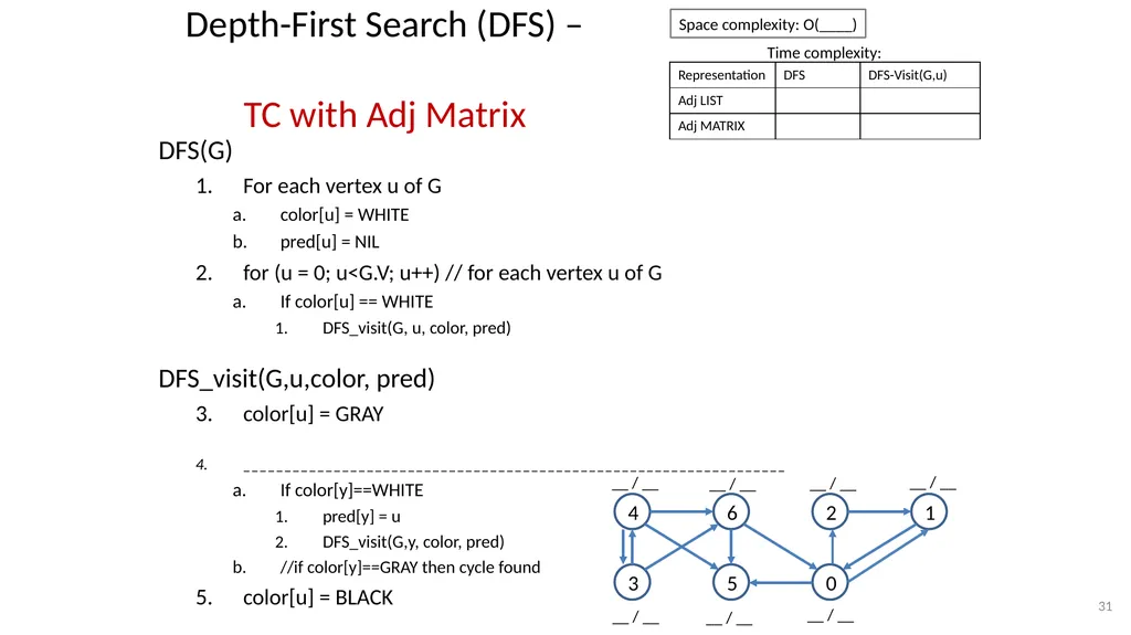
31
Depth-First Search (DFS) –
TC with Adj Matrix DFS(G)
For each vertex u of G
color[u] = WHITE
pred[u] = NIL
for (u = 0; u<G.V; u++) // for each vertex u of G
If color[u] == WHITE
DFS_visit(G, u, color, pred)
DFS_visit(G,u,color, pred)
color[u] = GRAY
__________________________________________________________________
If color[y]==WHITE
pred[y] = u
DFS_visit(G,y, color, pred)
//if color[y]==GRAY then cycle found
color[u] = BLACK 31 4 6 3 5 0 2 1 __ / __ __ / __ __ / __ __ / __ __ / __ __ / __ __ / __ Space complexity: O(____) Time complexity:<br>
For each vertex u of G
color[u] = WHITE
pred[u] = NIL
for (u = 0; u<G.V; u++) // for each vertex u of G
If color[u] == WHITE
DFS_visit(G, u, color, pred)
DFS_visit(G,u,color, pred)
color[u] = GRAY
__________________________________________________________________
If color[y]==WHITE
pred[y] = u
DFS_visit(G,y, color, pred)
//if color[y]==GRAY then cycle found
color[u] = BLACK 31 4 6 3 5 0 2 1 __ / __ __ / __ __ / __ __ / __ __ / __ __ / __ __ / __ Space complexity: O(____) Time complexity:<br>
32
32<br>
33
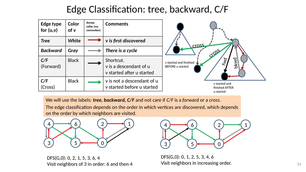
Edge Classification: tree, backward, C/F We will use the labels: tree, backward, C/F and not care if C/F is a forward or a cross.
The edge classification depends on the order in which vertices are discovered, which depends on the order by which neighbors are visited. 33 4 6 3 5 0 2 1 4 6 3 5 0 2 1 DFS(G,0): 0, 2, 1, 5, 3, 6, 4
Visit neighbors of 3 in order: 6 and then 4 DFS(G,0): 0, 1, 2, 5, 3, 4, 6
Visit neighbors in increasing order. v started and finished BEFORE u started v started and finished AFTER u started<br>
The edge classification depends on the order in which vertices are discovered, which depends on the order by which neighbors are visited. 33 4 6 3 5 0 2 1 4 6 3 5 0 2 1 DFS(G,0): 0, 2, 1, 5, 3, 6, 4
Visit neighbors of 3 in order: 6 and then 4 DFS(G,0): 0, 1, 2, 5, 3, 4, 6
Visit neighbors in increasing order. v started and finished BEFORE u started v started and finished AFTER u started<br>
34
Edge Classification for
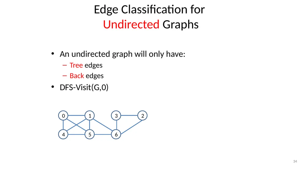
Undirected Graphs An undirected graph will only have:
Tree edges
Back edges
DFS-Visit(G,0) 34<br>
Tree edges
Back edges
DFS-Visit(G,0) 34<br>
35
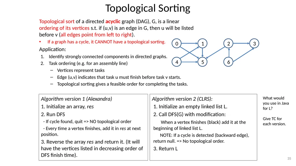
Topological Sorting Topological sort of a directed acyclic graph (DAG), G, is a linear ordering of its vertices s.t. if (u,v) is an edge in G, then u will be listed before v (all edges point from left to right).
If a graph has a cycle, it CANNOT have a topological sorting.
Application:
Identify strongly connected components in directed graphs.
Task ordering (e.g. for an assembly line)
Vertices represent tasks
Edge (u,v) indicates that task u must finish before task v starts.
Topological sorting gives a feasible order for completing the tasks. 35 Algorithm version 1 (Alexandra)
1. Initialize an array, res
2. Run DFS
- If cycle found, quit => NO topological order
- Every time a vertex finishes, add it in res at next position.
3. Reverse the array res and return it. (It will have the vertices listed in decreasing order of DFS finish time). Algorithm version 2 (CLRS):
1. Initialize an empty linked list L.
2. Call DFS(G) with modification:
When a vertex finishes (black) add it at the beginning of linked list L.
NOTE: If a cycle is detected (backward edge), return null. => No topological order.
3. Return L 0 1 4 5 6 2 3 What would you use in Java for L?
Give TC for each version.<br>
If a graph has a cycle, it CANNOT have a topological sorting.
Application:
Identify strongly connected components in directed graphs.
Task ordering (e.g. for an assembly line)
Vertices represent tasks
Edge (u,v) indicates that task u must finish before task v starts.
Topological sorting gives a feasible order for completing the tasks. 35 Algorithm version 1 (Alexandra)
1. Initialize an array, res
2. Run DFS
- If cycle found, quit => NO topological order
- Every time a vertex finishes, add it in res at next position.
3. Reverse the array res and return it. (It will have the vertices listed in decreasing order of DFS finish time). Algorithm version 2 (CLRS):
1. Initialize an empty linked list L.
2. Call DFS(G) with modification:
When a vertex finishes (black) add it at the beginning of linked list L.
NOTE: If a cycle is detected (backward edge), return null. => No topological order.
3. Return L 0 1 4 5 6 2 3 What would you use in Java for L?
Give TC for each version.<br>
36
Directed Acyclic Graphs (DAG)
&
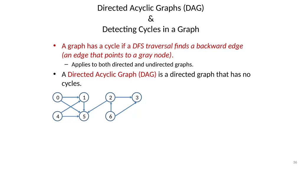
Detecting Cycles in a Graph A graph has a cycle if a DFS traversal finds a backward edge (an edge that points to a gray node).
Applies to both directed and undirected graphs.
A Directed Acyclic Graph (DAG) is a directed graph that has no cycles. 36 0 1 4 5 6 2 3<br>
Applies to both directed and undirected graphs.
A Directed Acyclic Graph (DAG) is a directed graph that has no cycles. 36 0 1 4 5 6 2 3<br>
37
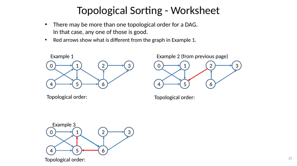
Topological Sorting - Worksheet 37 0 1 4 5 6 2 3 0 1 4 5 6 2 3 Example 2 (from previous page) Example 1 Topological order: Topological order: There may be more than one topological order for a DAG. In that case, any one of those is good.
Red arrows show what is different from the graph in Example 1. 0 1 4 5 6 2 3 Example 3 Topological order:<br>
Red arrows show what is different from the graph in Example 1. 0 1 4 5 6 2 3 Example 3 Topological order:<br>
38
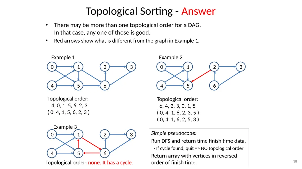
Topological Sorting - Answer 38 0 1 4 5 6 2 3 0 1 4 5 6 2 3 Example 2 Example 1 Topological order:
4, 0, 1, 5, 6, 2, 3
( 0, 4, 1, 5, 6, 2, 3 ) Topological order:
6, 4, 2, 3, 0, 1, 5
( 0, 4, 1, 6, 2, 3, 5 )
( 0, 4, 1, 6, 2, 5, 3 ) 0 1 4 5 6 2 3 Example 3 Topological order: none. It has a cycle. Simple pseudocode:
Run DFS and return time finish time data.
- If cycle found, quit => NO topological order
Return array with vertices in reversed order of finish time. There may be more than one topological order for a DAG. In that case, any one of those is good.
Red arrows show what is different from the graph in Example 1.<br>
4, 0, 1, 5, 6, 2, 3
( 0, 4, 1, 5, 6, 2, 3 ) Topological order:
6, 4, 2, 3, 0, 1, 5
( 0, 4, 1, 6, 2, 3, 5 )
( 0, 4, 1, 6, 2, 5, 3 ) 0 1 4 5 6 2 3 Example 3 Topological order: none. It has a cycle. Simple pseudocode:
Run DFS and return time finish time data.
- If cycle found, quit => NO topological order
Return array with vertices in reversed order of finish time. There may be more than one topological order for a DAG. In that case, any one of those is good.
Red arrows show what is different from the graph in Example 1.<br>
39
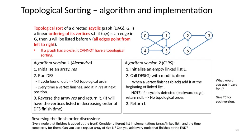
Topological Sorting – algorithm and implementation Topological sort of a directed acyclic graph (DAG), G, is a linear ordering of its vertices s.t. if (u,v) is an edge in G, then u will be listed before v (all edges point from left to right).
If a graph has a cycle, it CANNOT have a topological sorting. 39 Algorithm version 1 (Alexandra)
1. Initialize an array, res
2. Run DFS
- If cycle found, quit => NO topological order
- Every time a vertex finishes, add it in res at next position.
3. Reverse the array res and return it. (It will have the vertices listed in decreasing order of DFS finish time). Algorithm version 2 (CLRS):
1. Initialize an empty linked list L.
2. Call DFS(G) with modification:
When a vertex finishes (black) add it at the beginning of linked list L.
NOTE: If a cycle is detected (backward edge), return null. => No topological order.
3. Return L 0 1 4 5 6 2 3 What would you use in Java for L?
Give TC for each version. Reversing the finish order discussion:
(Every node that finishes is added at the front) Consider different list implementations (array/linked list), and the time complexity for them. Can you use a regular array of size N? Can you add every node that finishes at the END?<br>
If a graph has a cycle, it CANNOT have a topological sorting. 39 Algorithm version 1 (Alexandra)
1. Initialize an array, res
2. Run DFS
- If cycle found, quit => NO topological order
- Every time a vertex finishes, add it in res at next position.
3. Reverse the array res and return it. (It will have the vertices listed in decreasing order of DFS finish time). Algorithm version 2 (CLRS):
1. Initialize an empty linked list L.
2. Call DFS(G) with modification:
When a vertex finishes (black) add it at the beginning of linked list L.
NOTE: If a cycle is detected (backward edge), return null. => No topological order.
3. Return L 0 1 4 5 6 2 3 What would you use in Java for L?
Give TC for each version. Reversing the finish order discussion:
(Every node that finishes is added at the front) Consider different list implementations (array/linked list), and the time complexity for them. Can you use a regular array of size N? Can you add every node that finishes at the END?<br>
40
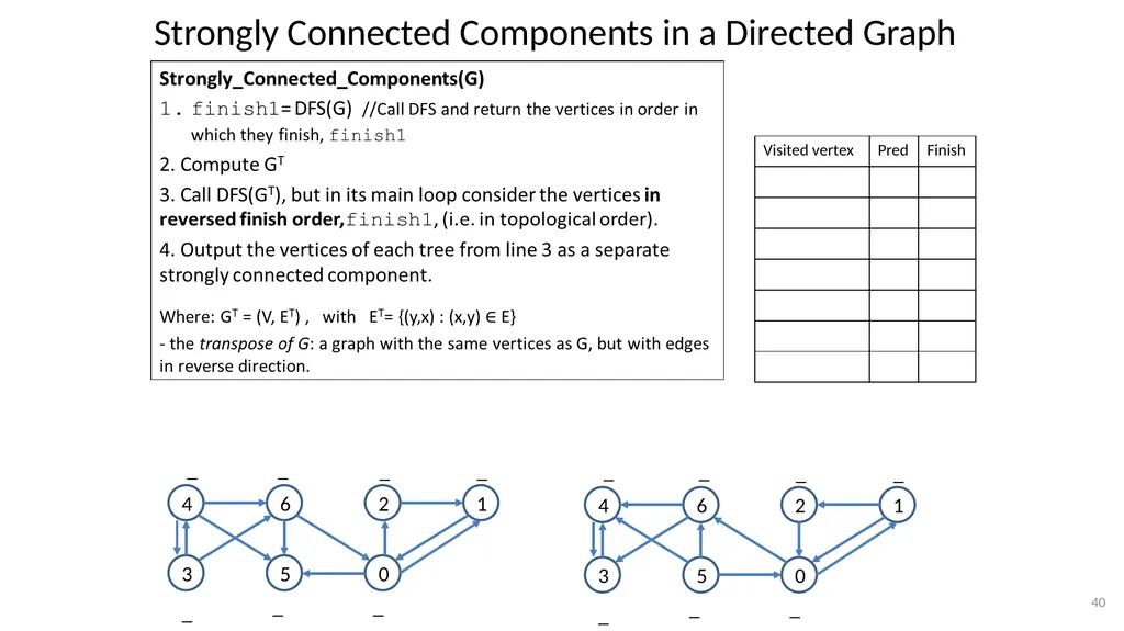
40 4 6 3 5 0 2 1 _ _ _ _ _ _ _ 4 6 3 5 0 2 1 _ _ _ _ _ _ _ Strongly Connected Components in a Directed Graph<br>
41
Applications of Strongly Connected Components (SCC) Simplify graph: collapse every SCC in one node
From stackoverflow (https://stackoverflow.com/questions/11212676/what-are-strongly-connected-components-used-for)
Model checking - “model checking is applied widely in the industry - especially for proving correctness of hardware components.”
Vehicle routing applications – “A road network can be modeled as a directed graph, with vertices being intersections, and arcs being directed road segments or individual lanes. If the graph isn't Strongly Connected, then vehicles can get trapped in a certain part of the graph (i.e. they can get in, but not get out).”
From Wikipedia (https://en.wikipedia.org/wiki/Strongly_connected_component)
SCC “may be used to solve 2-satisfiability problems (systems of Boolean variables with constraints on the values of pairs of variables)”
From neo4j (https://neo4j.com/docs/graph-algorithms/current/labs-algorithms/strongly-connected-components/)
“In the analysis of powerful transnational corporations, SCC can be used to find the set of firms in which every member owns directly and/or indirectly owns shares in every other member. Although it has benefits, such as reducing transaction costs and increasing trust, this type of structure can weaken market competition.”
“SCC can be used to compute the connectivity of different network configurations when measuring routing performance in multi hop wireless networks”
“applications in cell methods for the numerical study of discrete dynamical systems” https://math.stackexchange.com/questions/32041/uses-of-strongly-connected-components 41<br>
From stackoverflow (https://stackoverflow.com/questions/11212676/what-are-strongly-connected-components-used-for)
Model checking - “model checking is applied widely in the industry - especially for proving correctness of hardware components.”
Vehicle routing applications – “A road network can be modeled as a directed graph, with vertices being intersections, and arcs being directed road segments or individual lanes. If the graph isn't Strongly Connected, then vehicles can get trapped in a certain part of the graph (i.e. they can get in, but not get out).”
From Wikipedia (https://en.wikipedia.org/wiki/Strongly_connected_component)
SCC “may be used to solve 2-satisfiability problems (systems of Boolean variables with constraints on the values of pairs of variables)”
From neo4j (https://neo4j.com/docs/graph-algorithms/current/labs-algorithms/strongly-connected-components/)
“In the analysis of powerful transnational corporations, SCC can be used to find the set of firms in which every member owns directly and/or indirectly owns shares in every other member. Although it has benefits, such as reducing transaction costs and increasing trust, this type of structure can weaken market competition.”
“SCC can be used to compute the connectivity of different network configurations when measuring routing performance in multi hop wireless networks”
“applications in cell methods for the numerical study of discrete dynamical systems” https://math.stackexchange.com/questions/32041/uses-of-strongly-connected-components 41<br>
42
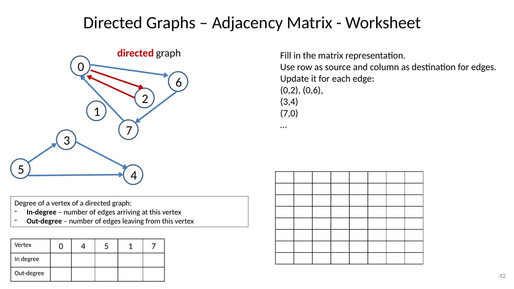
Directed Graphs – Adjacency Matrix - Worksheet 42 Degree of a vertex of a directed graph:
In-degree – number of edges arriving at this vertex
Out-degree – number of edges leaving from this vertex Fill in the matrix representation.
Use row as source and column as destination for edges.
Update it for each edge:
(0,2), (0,6),
(3,4)
(7,0)
…<br>
In-degree – number of edges arriving at this vertex
Out-degree – number of edges leaving from this vertex Fill in the matrix representation.
Use row as source and column as destination for edges.
Update it for each edge:
(0,2), (0,6),
(3,4)
(7,0)
…<br>
43
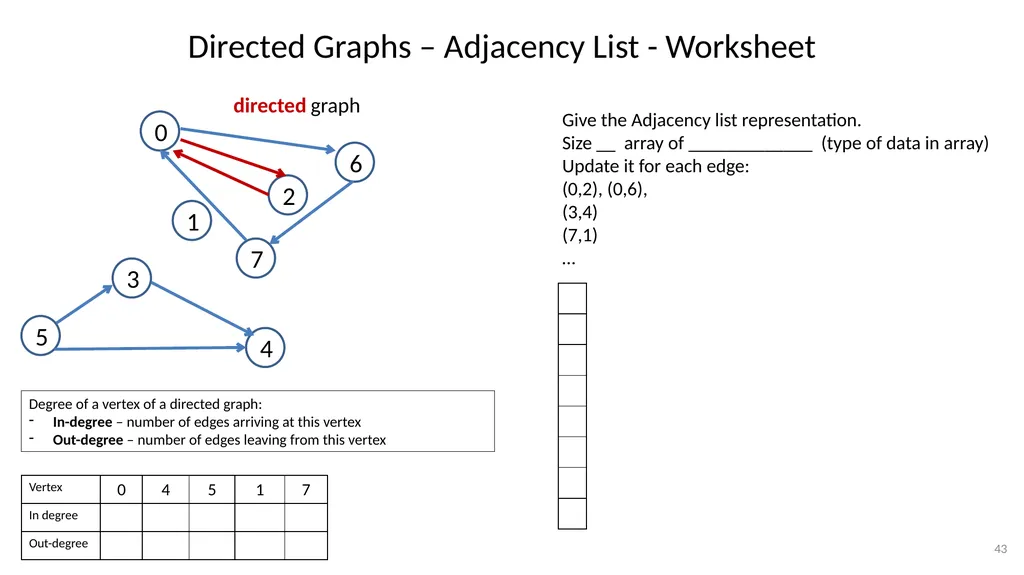
Directed Graphs – Adjacency List - Worksheet 43 Degree of a vertex of a directed graph:
In-degree – number of edges arriving at this vertex
Out-degree – number of edges leaving from this vertex Give the Adjacency list representation.
Size __ array of _____________ (type of data in array)
Update it for each edge:
(0,2), (0,6),
(3,4)
(7,1)
…<br>
In-degree – number of edges arriving at this vertex
Out-degree – number of edges leaving from this vertex Give the Adjacency list representation.
Size __ array of _____________ (type of data in array)
Update it for each edge:
(0,2), (0,6),
(3,4)
(7,1)
…<br>
44
Extra Slides 44<br>
45
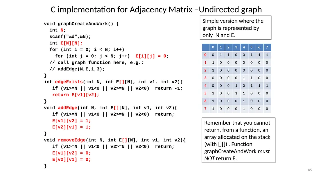
C implementation for Adjacency Matrix –Undirected graph void graphCreateAndWork() {
int N;
scanf("%d",&N);
int E[N][N];
for (int i = 0; i < N; i++)
for (int j = 0; j < N; j++) E[i][j] = 0;
// call graph function here, e.g.:
// addEdge(N,E,1,3);
}
int edgeExists(int N, int E[][N], int v1, int v2){
if (v1>=N || v1<0 || v2>=N || v2<0) return -1;
return E[v1][v2];
}
void addEdge(int N, int E[][N], int v1, int v2){
if (v1>=N || v1<0 || v2>=N || v2<0) return;
E[v1][v2] = 1;
E[v2][v1] = 1;
}
void removeEdge(int N, int E[][N], int v1, int v2){
if (v1>=N || v1<0 || v2>=N || v2<0) return;
E[v1][v2] = 0;
E[v2][v1] = 0;
} 45 Remember that you cannot return, from a function, an array allocated on the stack (with [][]) . Function graphCreateAndWork must NOT return E. Simple version where the graph is represented by only N and E.<br>
int N;
scanf("%d",&N);
int E[N][N];
for (int i = 0; i < N; i++)
for (int j = 0; j < N; j++) E[i][j] = 0;
// call graph function here, e.g.:
// addEdge(N,E,1,3);
}
int edgeExists(int N, int E[][N], int v1, int v2){
if (v1>=N || v1<0 || v2>=N || v2<0) return -1;
return E[v1][v2];
}
void addEdge(int N, int E[][N], int v1, int v2){
if (v1>=N || v1<0 || v2>=N || v2<0) return;
E[v1][v2] = 1;
E[v2][v1] = 1;
}
void removeEdge(int N, int E[][N], int v1, int v2){
if (v1>=N || v1<0 || v2>=N || v2<0) return;
E[v1][v2] = 0;
E[v2][v1] = 0;
} 45 Remember that you cannot return, from a function, an array allocated on the stack (with [][]) . Function graphCreateAndWork must NOT return E. Simple version where the graph is represented by only N and E.<br>
46
DFS with time stamps Next, DFS with ‘time stamps’ of when a node u was first discovered (d[u]) and the time when the algorithm finished processing that node (finish[u]).
The time stamps are needed for:
Topological sorting
Finding strongly connected components
edge labeling (to distinguish between forward and cross edges)
tree edge
backward edge
forward edge
cross edge
The following pseudo-code does not specify all the details of the implementation 46<br>
The time stamps are needed for:
Topological sorting
Finding strongly connected components
edge labeling (to distinguish between forward and cross edges)
tree edge
backward edge
forward edge
cross edge
The following pseudo-code does not specify all the details of the implementation 46<br>
47
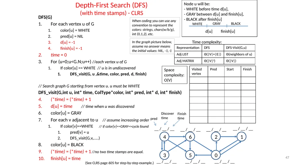
Depth-First Search (DFS)
(with time stamps) - CLRS DFS(G)
For each vertex u of G
color[u] = WHITE
pred[u] = NIL
d[u] = -1
finish[u] = -1
time = 0
For (u=0;u<G.N;u++) //each vertex u of G
If color[u] == WHITE // u is in undiscovered
DFS_visit(G, u ,&time, color, pred, d, finish)
// Search graph G starting from vertex u. u must be WHITE
DFS_visit(G,int u, int* time, ColType*color, int* pred, int* d, int* finish)
(*time) = (*time) + 1
d[u] = time // time when u was discovered
color[u] = GRAY
For each v adjacent to u // assume increasing order
If color[v]==WHITE // if color[v]==GRAY=>cycle found
pred[v] = u
DFS_visit(G,v,…..)
color[u] = BLACK
(*time) = (*time) + 1 //no two time stamps are equal.
finish[u] = time 47 4 6 3 5 0 2 1 Node u will be:
- WHITE before time d[u],
- GRAY between d[u] and finish[u],
- BLACK after finish[u] (See CLRS page 605 for step-by-step example.) __ / __ / __ Discover
time Finish time __ / __ / __ __ / __ / __ __ / __ / __ pred __ / __ / __ __ / __ / __ __ / __ / __ When coding you can use any convention to represent the colors: strings, chars(w/b/g), int (0,1,2), etc. In the graph picture below, assume no answer means the initial values: NIL, -1,-1 Space complexity: O(V) Time complexity:<br>
For each vertex u of G
color[u] = WHITE
pred[u] = NIL
d[u] = -1
finish[u] = -1
time = 0
For (u=0;u<G.N;u++) //each vertex u of G
If color[u] == WHITE // u is in undiscovered
DFS_visit(G, u ,&time, color, pred, d, finish)
// Search graph G starting from vertex u. u must be WHITE
DFS_visit(G,int u, int* time, ColType*color, int* pred, int* d, int* finish)
(*time) = (*time) + 1
d[u] = time // time when u was discovered
color[u] = GRAY
For each v adjacent to u // assume increasing order
If color[v]==WHITE // if color[v]==GRAY=>cycle found
pred[v] = u
DFS_visit(G,v,…..)
color[u] = BLACK
(*time) = (*time) + 1 //no two time stamps are equal.
finish[u] = time 47 4 6 3 5 0 2 1 Node u will be:
- WHITE before time d[u],
- GRAY between d[u] and finish[u],
- BLACK after finish[u] (See CLRS page 605 for step-by-step example.) __ / __ / __ Discover
time Finish time __ / __ / __ __ / __ / __ __ / __ / __ pred __ / __ / __ __ / __ / __ __ / __ / __ When coding you can use any convention to represent the colors: strings, chars(w/b/g), int (0,1,2), etc. In the graph picture below, assume no answer means the initial values: NIL, -1,-1 Space complexity: O(V) Time complexity:<br>
48
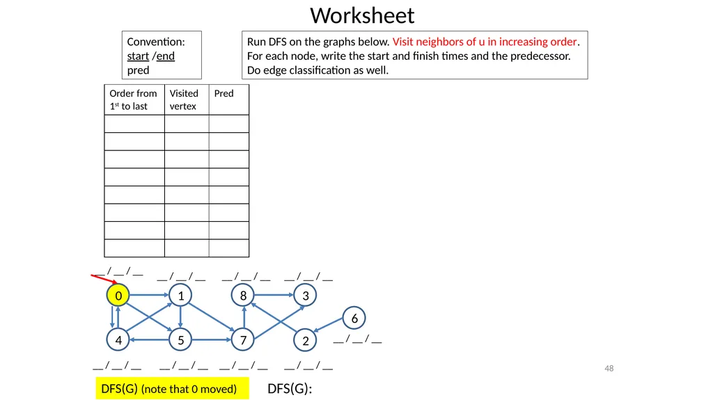
DFS(G): 48 0 1 4 5 7 8 3 DFS(G) (note that 0 moved) Convention:
start /end
pred Run DFS on the graphs below. Visit neighbors of u in increasing order.
For each node, write the start and finish times and the predecessor.
Do edge classification as well. Worksheet 2 6 __ / __ / __ __ / __ / __ __ / __ / __ __ / __ / __ __ / __ / __ __ / __ / __ __ / __ / __ __ / __ / __ __ / __ / __<br>
start /end
pred Run DFS on the graphs below. Visit neighbors of u in increasing order.
For each node, write the start and finish times and the predecessor.
Do edge classification as well. Worksheet 2 6 __ / __ / __ __ / __ / __ __ / __ / __ __ / __ / __ __ / __ / __ __ / __ / __ __ / __ / __ __ / __ / __ __ / __ / __<br>
49
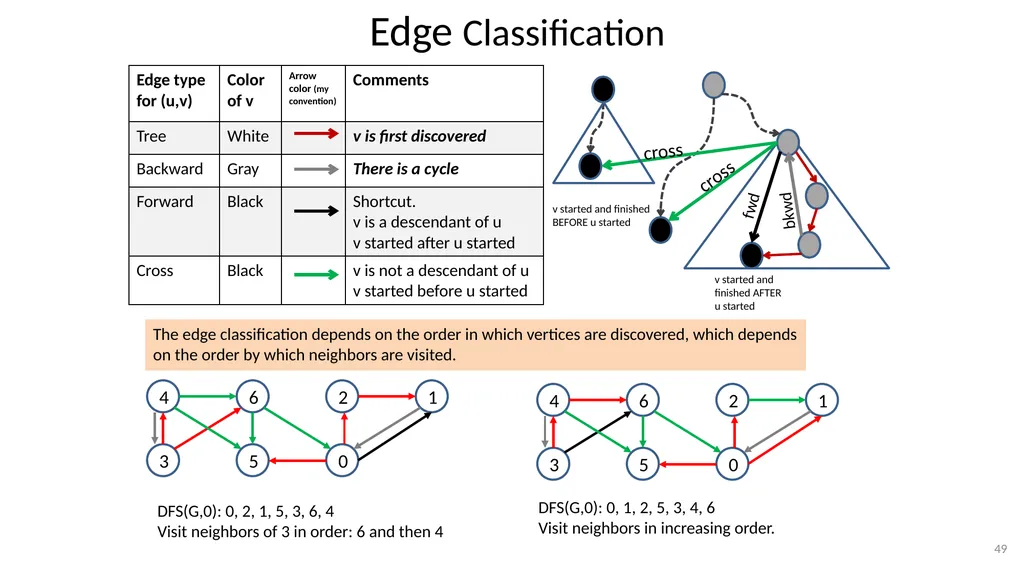
Edge Classification The edge classification depends on the order in which vertices are discovered, which depends on the order by which neighbors are visited. 49 4 6 3 5 0 2 1 4 6 3 5 0 2 1 DFS(G,0): 0, 2, 1, 5, 3, 6, 4
Visit neighbors of 3 in order: 6 and then 4 DFS(G,0): 0, 1, 2, 5, 3, 4, 6
Visit neighbors in increasing order. v started and finished BEFORE u started v started and finished AFTER u started<br>
Visit neighbors of 3 in order: 6 and then 4 DFS(G,0): 0, 1, 2, 5, 3, 4, 6
Visit neighbors in increasing order. v started and finished BEFORE u started v started and finished AFTER u started<br>
50
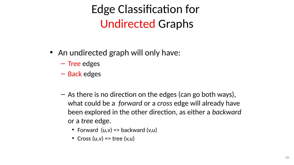
Edge Classification for
Undirected Graphs An undirected graph will only have:
Tree edges
Back edges
As there is no direction on the edges (can go both ways), what could be a forward or a cross edge will already have been explored in the other direction, as either a backward or a tree edge.
Forward (u,v) => backward (v,u)
Cross (u,v) => tree (v,u) 50<br>
Tree edges
Back edges
As there is no direction on the edges (can go both ways), what could be a forward or a cross edge will already have been explored in the other direction, as either a backward or a tree edge.
Forward (u,v) => backward (v,u)
Cross (u,v) => tree (v,u) 50<br>
51
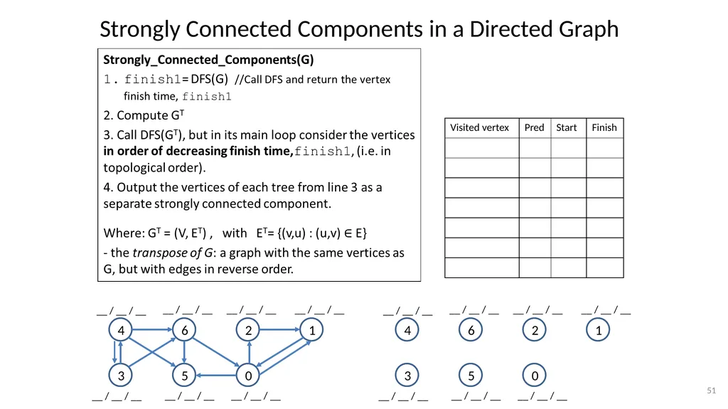
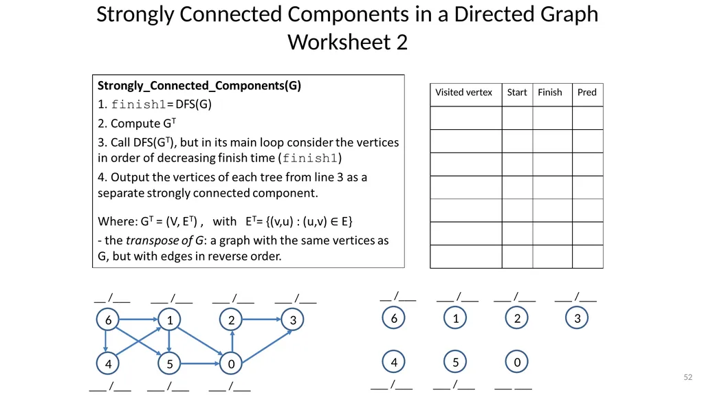
Strongly Connected Components in a Directed Graph 51 4 6 3 5 0 2 1 __ / __ / __ __ / __ / __ __ / __ / __ __ / __ / __ __ / __ / __ __ / __ / __ __ / __ / __ 4 6 3 5 0 2 1 __ / __ / __ __ / __ / __ __ / __ / __ __ / __ / __ __ / __ / __ __ / __ / __ __ / __ / __<br>
52
Strongly Connected Components in a Directed Graph
Worksheet 2 52 6 1 4 5 0 2 3 __ /___ ___ /___ ___ /___ ___ /___ ___ /___ ___ /___ ___ /___ 6 1 4 5 0 2 3 __ /___ ___ /___ ___ /___ ___ /___ ___ ___ ___ /___ ___ /___<br>
53
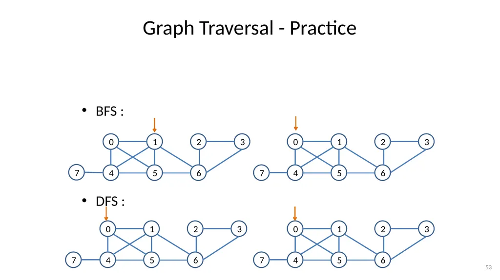
Graph Traversal - Practice DFS : 53 0 1 4 5 6 2 3 0 1 4 5 6 2 3 0 1 4 5 6 2 3 7 0 1 4 5 6 2 3 BFS : 7 7 7<br>
54
Graph Traversal DFS traversal examples. 54 0 1 4 5 6 2 3 BFS traversal examples: 0 1 4 5 6 2 3 0 1 4 5 6 2 3 7 0 1 4 5 6 2 3 7 7 7 For both DFS and BFS the resulting trees depend on the order in which neighbors are visited.<br>
55
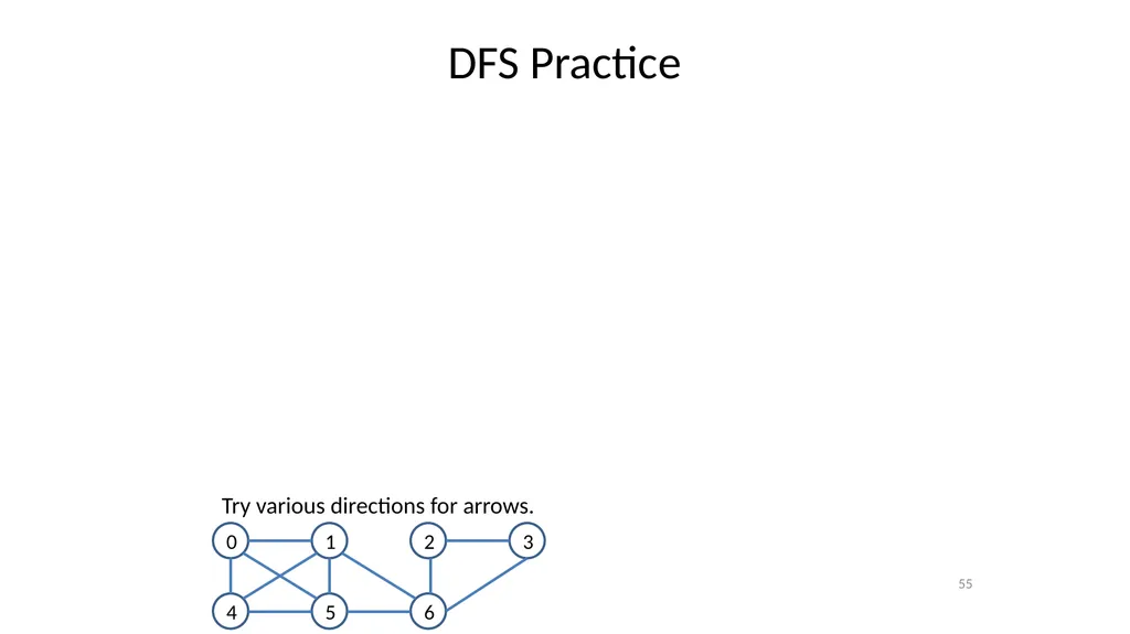
DFS Practice 55 0 1 4 5 6 2 3 Try various directions for arrows.<br>
56
Extra Material – Not required
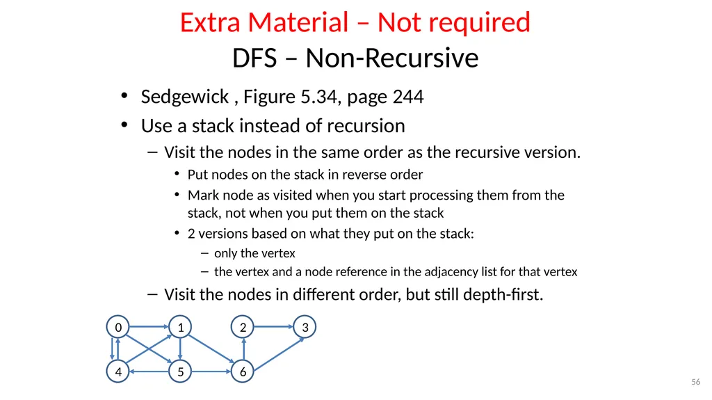
DFS – Non-Recursive Sedgewick , Figure 5.34, page 244
Use a stack instead of recursion
Visit the nodes in the same order as the recursive version.
Put nodes on the stack in reverse order
Mark node as visited when you start processing them from the stack, not when you put them on the stack
2 versions based on what they put on the stack:
only the vertex
the vertex and a node reference in the adjacency list for that vertex
Visit the nodes in different order, but still depth-first. 56 0 1 4 5 6 2 3<br>
Use a stack instead of recursion
Visit the nodes in the same order as the recursive version.
Put nodes on the stack in reverse order
Mark node as visited when you start processing them from the stack, not when you put them on the stack
2 versions based on what they put on the stack:
only the vertex
the vertex and a node reference in the adjacency list for that vertex
Visit the nodes in different order, but still depth-first. 56 0 1 4 5 6 2 3<br>