
Intermediate-value theorem Introduction In this
Description: Intermediate-value theorem Introduction In this topic, we will Review the intermediate-value theorem Look at some theorems that result from this theorem Look at applications of these new theorems Discuss how we will apply these theorems in
Related Topics
Download Presentation
"Intermediate-value theorem Introduction In this" is the property of its rightful owner. Permission is granted to download and print the materials on this website for personal, non-commercial use only, and to display it on your personal computer provided you do not modify the materials and that you retain all copyright notices contained in the materials. By downloading content from our website, you accept the terms of this agreement.
Presentation Transcript
slide1. Intermediate-value theorem<br>
slide2. Introduction In this topic, we will
Review the intermediate-value theorem
Look at some theorems that result from this theorem
Look at applications of these new theorems
Discuss how we will apply these theorems in this course Intermediate-value theorem 2<br>
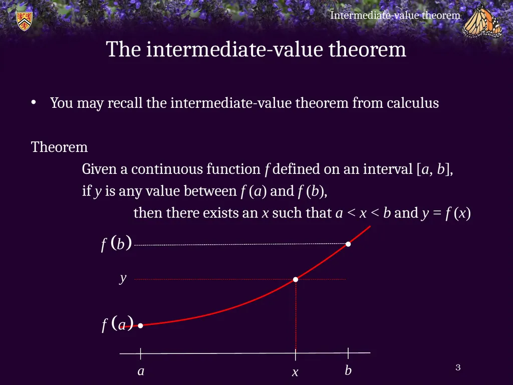
slide3. The intermediate-value theorem You may recall the intermediate-value theorem from calculus
Theorem
Given a continuous function f defined on an interval [a, b],
if y is any value between f (a) and f (b),
then there exists an x such that a < x < b and y = f (x) Intermediate-value theorem 3 a b x y<br>
slide4. Application Theorem
Given a continuous function f defined on an interval [a, b]
where f (a) and f (b) have opposite signs,
then there exists a root x such that a < x < b
Proof:
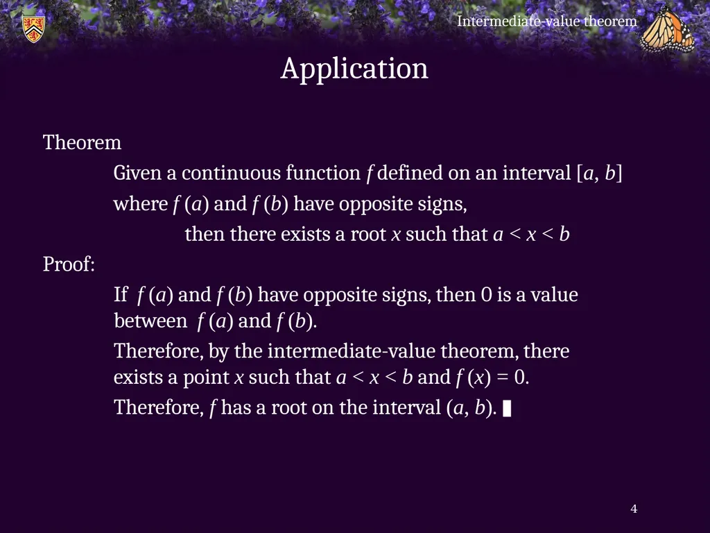
If f (a) and f (b) have opposite signs, then 0 is a value between f (a) and f (b).
Therefore, by the intermediate-value theorem, there exists a point x such that a < x < b and f (x) = 0.
Therefore, f has a root on the interval (a, b). ▮ Intermediate-value theorem 4<br>
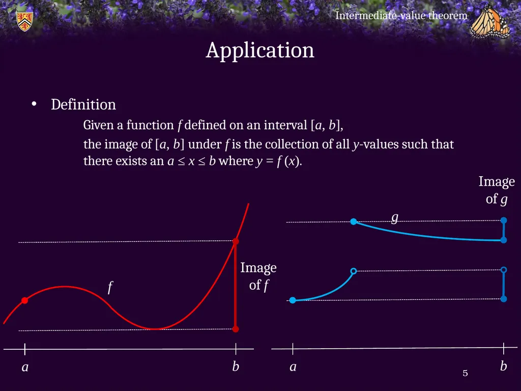
slide5. Application Definition
Given a function f defined on an interval [a, b],
the image of [a, b] under f is the collection of all y-values such that there exists an a ≤ x ≤ b where y = f (x). Intermediate-value theorem 5 a b f a b g Image
of g Image
of f<br>
slide6. Application Theorem
Given a continuous function f defined on an interval [a, b]
the image of [a, b] under f is also an interval.
Proof:
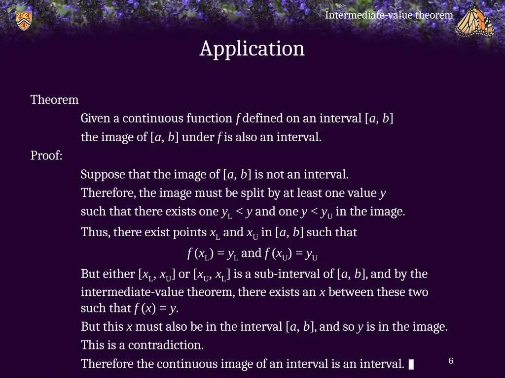
Suppose that the image of [a, b] is not an interval.
Therefore, the image must be split by at least one value y
such that there exists one yL < y and one y < yU in the image.
Thus, there exist points xL and xU in [a, b] such that
f (xL) = yL and f (xU) = yU
But either [xL, xU] or [xU, xL] is a sub-interval of [a, b], and by the intermediate-value theorem, there exists an x between these two such that f (x) = y.
But this x must also be in the interval [a, b], and so y is in the image.
This is a contradiction.
Therefore the continuous image of an interval is an interval. ▮ Intermediate-value theorem 6<br>
slide7. Application Theorem
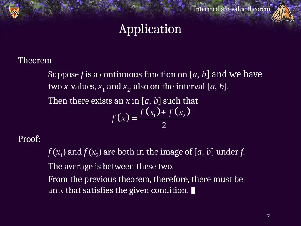
Suppose f is a continuous function on [a, b] and we have two x-values, x1 and x2, also on the interval [a, b].
Then there exists an x in [a, b] such that
Proof:
f (x1) and f (x2) are both in the image of [a, b] under f.
The average is between these two.
From the previous theorem, therefore, there must be an x that satisfies the given condition. ▮ Intermediate-value theorem 7<br>
slide8. Application Theorem
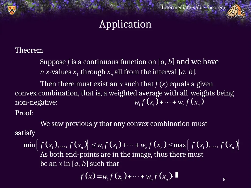
Suppose f is a continuous function on [a, b] and we have n x-values x1 through xn all from the interval [a, b].
Then there must exist an x such that f (x) equals a given convex combination, that is, a weighted average with all weights being non-negative:
Proof:
We saw previously that any convex combination must satisfy
As both end-points are in the image, thus there must be an x in [a, b] such that
. ▮ Intermediate-value theorem 8<br>
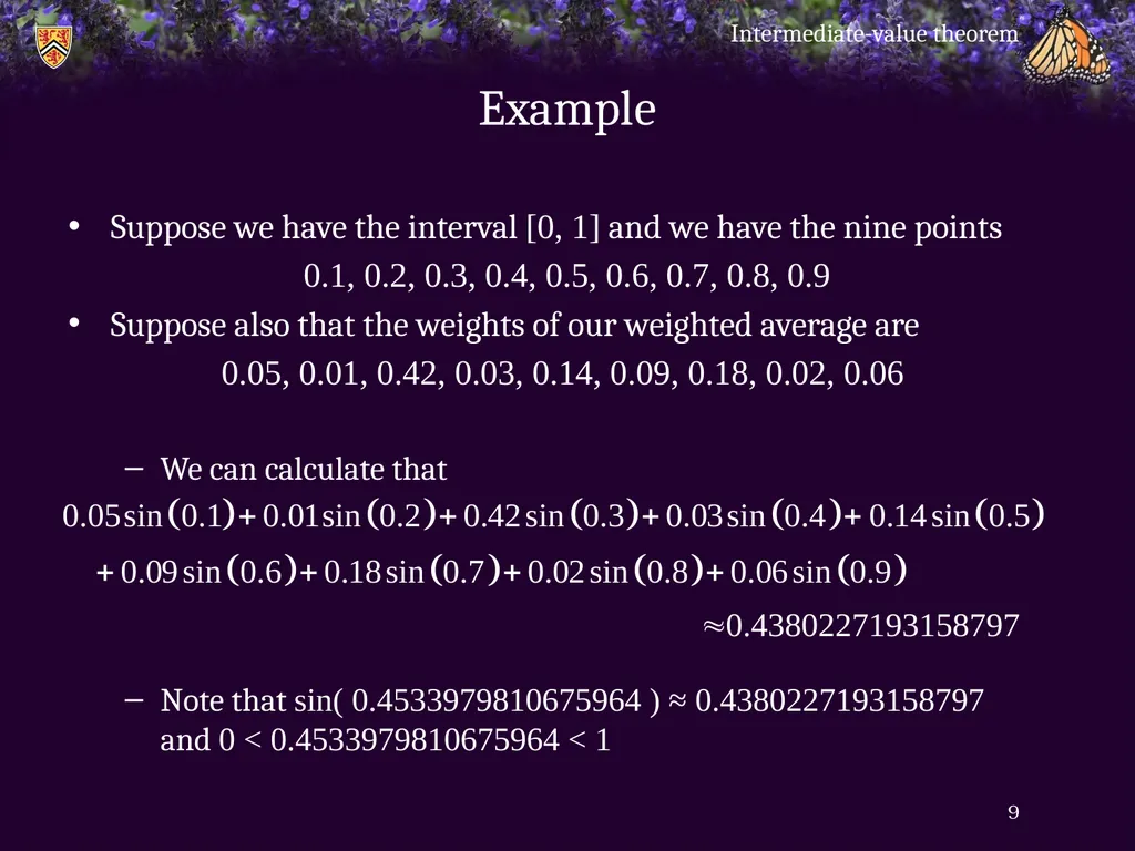
slide9. Example Suppose we have the interval [0, 1] and we have the nine points
0.1, 0.2, 0.3, 0.4, 0.5, 0.6, 0.7, 0.8, 0.9
Suppose also that the weights of our weighted average are
0.05, 0.01, 0.42, 0.03, 0.14, 0.09, 0.18, 0.02, 0.06
We can calculate that
Note that sin( 0.4533979810675964 ) ≈ 0.4380227193158797 and 0 < 0.4533979810675964 < 1 Intermediate-value theorem 9<br>
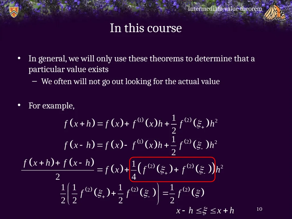
slide10. In this course In general, we will only use these theorems to determine that a particular value exists
We often will not go out looking for the actual value
For example, Intermediate-value theorem 10<br>
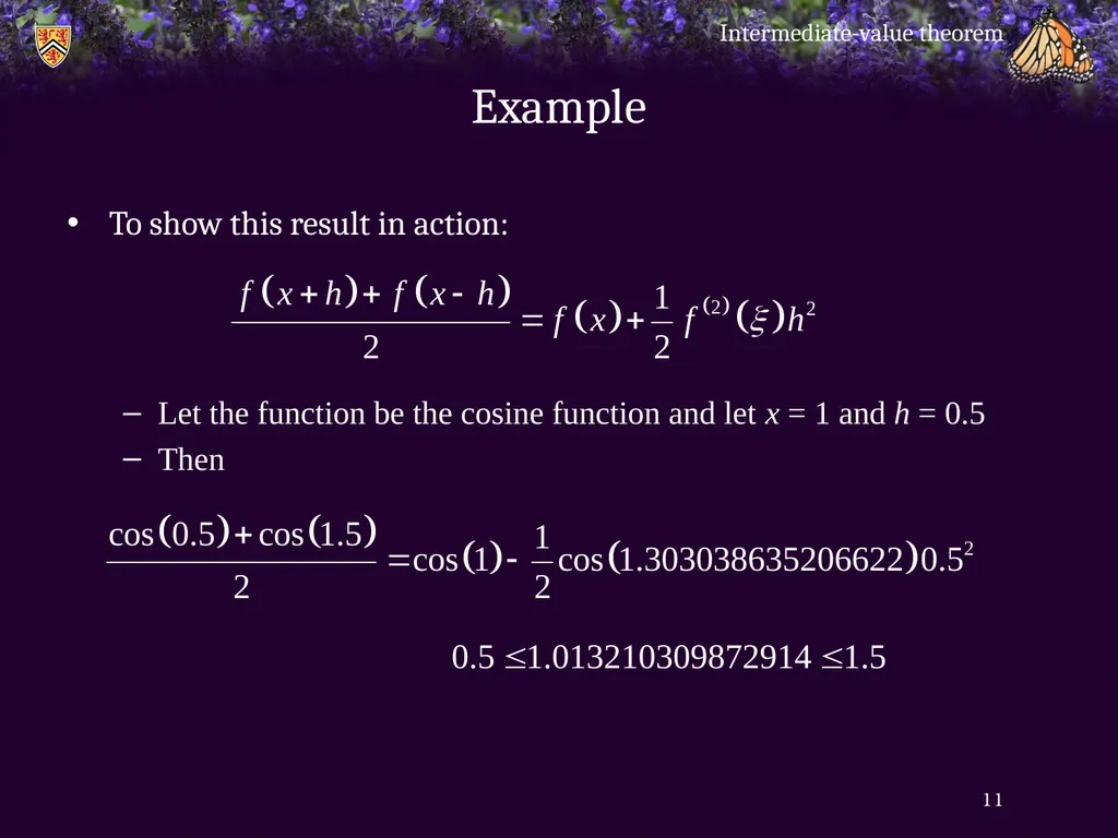
slide11. Example To show this result in action:
Let the function be the cosine function and let x = 1 and h = 0.5
Then Intermediate-value theorem 11<br>
slide12. Summary Following this topic, you now
Have reviewed the intermediate-value theorem
Seen a few theorems that are a consequence of that theorem
Seen a few applications these theorems and how these will be used in this course Intermediate-value theorem 12<br>
slide13. References [1] https://en.wikipedia.org/wiki/Intermediate_value_theorem Intermediate-value theorem 13<br>
slide14. Acknowledgments Mayuresh Gaikwad for noting an error on p.9, which propagated to p.10.
Tazik Shahjahan for pointing out typos. Intermediate-value theorem 14<br>
slide15. Colophon These slides were prepared using the Cambria typeface. Mathematical equations use Times New Roman, and source code is presented using Consolas. Mathematical equations are prepared in MathType by Design Science, Inc.
Examples may be formulated and checked using Maple by Maplesoft, Inc.
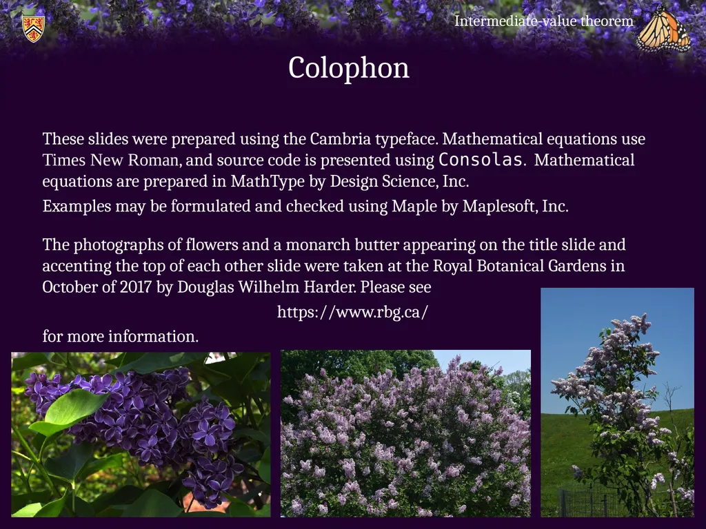
The photographs of flowers and a monarch butter appearing on the title slide and accenting the top of each other slide were taken at the Royal Botanical Gardens in October of 2017 by Douglas Wilhelm Harder. Please see
https://www.rbg.ca/
for more information. Intermediate-value theorem 15<br>
slide16. Disclaimer These slides are provided for the ece 204 Numerical methods course taught at the University of Waterloo. The material in it reflects the author’s best judgment in light of the information available to them at the time of preparation. Any reliance on these course slides by any party for any other purpose are the responsibility of such parties. The authors accept no responsibility for damages, if any, suffered by any party as a result of decisions made or actions based on these course slides for any other purpose than that for which it was intended. Intermediate-value theorem 16<br>
slide2. Introduction In this topic, we will
Review the intermediate-value theorem
Look at some theorems that result from this theorem
Look at applications of these new theorems
Discuss how we will apply these theorems in this course Intermediate-value theorem 2<br>
slide3. The intermediate-value theorem You may recall the intermediate-value theorem from calculus
Theorem
Given a continuous function f defined on an interval [a, b],
if y is any value between f (a) and f (b),
then there exists an x such that a < x < b and y = f (x) Intermediate-value theorem 3 a b x y<br>
slide4. Application Theorem
Given a continuous function f defined on an interval [a, b]
where f (a) and f (b) have opposite signs,
then there exists a root x such that a < x < b
Proof:
If f (a) and f (b) have opposite signs, then 0 is a value between f (a) and f (b).
Therefore, by the intermediate-value theorem, there exists a point x such that a < x < b and f (x) = 0.
Therefore, f has a root on the interval (a, b). ▮ Intermediate-value theorem 4<br>
slide5. Application Definition
Given a function f defined on an interval [a, b],
the image of [a, b] under f is the collection of all y-values such that there exists an a ≤ x ≤ b where y = f (x). Intermediate-value theorem 5 a b f a b g Image
of g Image
of f<br>
slide6. Application Theorem
Given a continuous function f defined on an interval [a, b]
the image of [a, b] under f is also an interval.
Proof:
Suppose that the image of [a, b] is not an interval.
Therefore, the image must be split by at least one value y
such that there exists one yL < y and one y < yU in the image.
Thus, there exist points xL and xU in [a, b] such that
f (xL) = yL and f (xU) = yU
But either [xL, xU] or [xU, xL] is a sub-interval of [a, b], and by the intermediate-value theorem, there exists an x between these two such that f (x) = y.
But this x must also be in the interval [a, b], and so y is in the image.
This is a contradiction.
Therefore the continuous image of an interval is an interval. ▮ Intermediate-value theorem 6<br>
slide7. Application Theorem
Suppose f is a continuous function on [a, b] and we have two x-values, x1 and x2, also on the interval [a, b].
Then there exists an x in [a, b] such that
Proof:
f (x1) and f (x2) are both in the image of [a, b] under f.
The average is between these two.
From the previous theorem, therefore, there must be an x that satisfies the given condition. ▮ Intermediate-value theorem 7<br>
slide8. Application Theorem
Suppose f is a continuous function on [a, b] and we have n x-values x1 through xn all from the interval [a, b].
Then there must exist an x such that f (x) equals a given convex combination, that is, a weighted average with all weights being non-negative:
Proof:
We saw previously that any convex combination must satisfy
As both end-points are in the image, thus there must be an x in [a, b] such that
. ▮ Intermediate-value theorem 8<br>
slide9. Example Suppose we have the interval [0, 1] and we have the nine points
0.1, 0.2, 0.3, 0.4, 0.5, 0.6, 0.7, 0.8, 0.9
Suppose also that the weights of our weighted average are
0.05, 0.01, 0.42, 0.03, 0.14, 0.09, 0.18, 0.02, 0.06
We can calculate that
Note that sin( 0.4533979810675964 ) ≈ 0.4380227193158797 and 0 < 0.4533979810675964 < 1 Intermediate-value theorem 9<br>
slide10. In this course In general, we will only use these theorems to determine that a particular value exists
We often will not go out looking for the actual value
For example, Intermediate-value theorem 10<br>
slide11. Example To show this result in action:
Let the function be the cosine function and let x = 1 and h = 0.5
Then Intermediate-value theorem 11<br>
slide12. Summary Following this topic, you now
Have reviewed the intermediate-value theorem
Seen a few theorems that are a consequence of that theorem
Seen a few applications these theorems and how these will be used in this course Intermediate-value theorem 12<br>
slide13. References [1] https://en.wikipedia.org/wiki/Intermediate_value_theorem Intermediate-value theorem 13<br>
slide14. Acknowledgments Mayuresh Gaikwad for noting an error on p.9, which propagated to p.10.
Tazik Shahjahan for pointing out typos. Intermediate-value theorem 14<br>
slide15. Colophon These slides were prepared using the Cambria typeface. Mathematical equations use Times New Roman, and source code is presented using Consolas. Mathematical equations are prepared in MathType by Design Science, Inc.
Examples may be formulated and checked using Maple by Maplesoft, Inc.
The photographs of flowers and a monarch butter appearing on the title slide and accenting the top of each other slide were taken at the Royal Botanical Gardens in October of 2017 by Douglas Wilhelm Harder. Please see
https://www.rbg.ca/
for more information. Intermediate-value theorem 15<br>
slide16. Disclaimer These slides are provided for the ece 204 Numerical methods course taught at the University of Waterloo. The material in it reflects the author’s best judgment in light of the information available to them at the time of preparation. Any reliance on these course slides by any party for any other purpose are the responsibility of such parties. The authors accept no responsibility for damages, if any, suffered by any party as a result of decisions made or actions based on these course slides for any other purpose than that for which it was intended. Intermediate-value theorem 16<br>