
INTRODUCTION TO Machine Learning 3rd Edition ETHEM
Description: INTRODUCTION TO Machine Learning 3rd Edition ETHEM ALPAYDIN The MIT Press, 2014 alpaydinboun.edu.tr http:www.cmpe.boun.edu.trethemi2ml3e Lecture Slides for CHAPTER 5: Multivariate Methods Multivariate Data 3 Multiple measurements
Related Topics
Download Presentation
"INTRODUCTION TO Machine Learning 3rd Edition ETHEM" is the property of its rightful owner. Permission is granted to download and print the materials on this website for personal, non-commercial use only, and to display it on your personal computer provided you do not modify the materials and that you retain all copyright notices contained in the materials. By downloading content from our website, you accept the terms of this agreement.
Presentation Transcript
slide1. INTRODUCTION
TO
Machine
Learning
3rd Edition ETHEM ALPAYDIN
© The MIT Press, 2014
alpaydin@boun.edu.tr
http://www.cmpe.boun.edu.tr/~ethem/i2ml3e Lecture Slides for<br>
slide2. CHAPTER 5: Multivariate Methods<br>
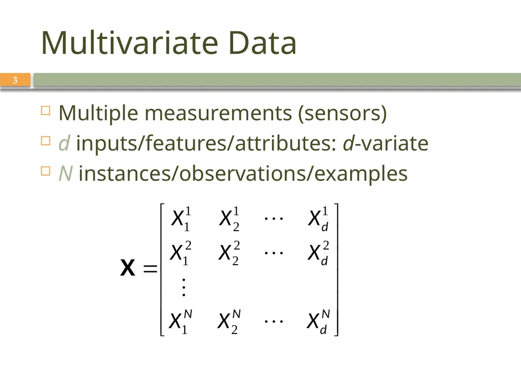
slide3. Multivariate Data 3 Multiple measurements (sensors)
d inputs/features/attributes: d-variate
N instances/observations/examples<br>
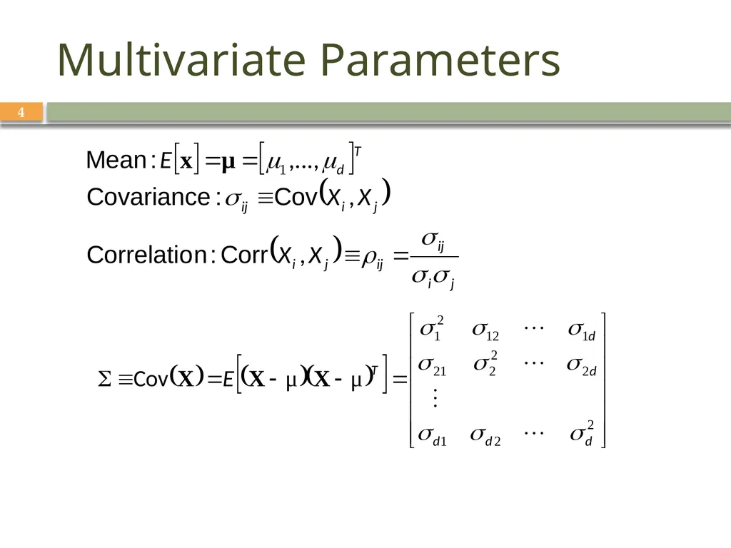
slide4. Multivariate Parameters 4<br>
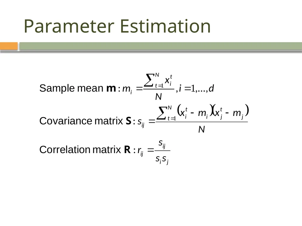
slide5. Parameter Estimation 5<br>
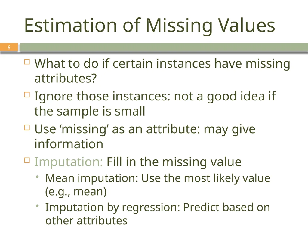
slide6. Estimation of Missing Values 6 What to do if certain instances have missing attributes?
Ignore those instances: not a good idea if the sample is small
Use ‘missing’ as an attribute: may give information
Imputation: Fill in the missing value
Mean imputation: Use the most likely value (e.g., mean)
Imputation by regression: Predict based on other attributes<br>
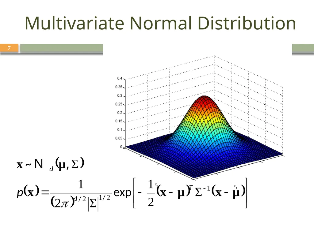
slide7. Multivariate Normal Distribution 7<br>
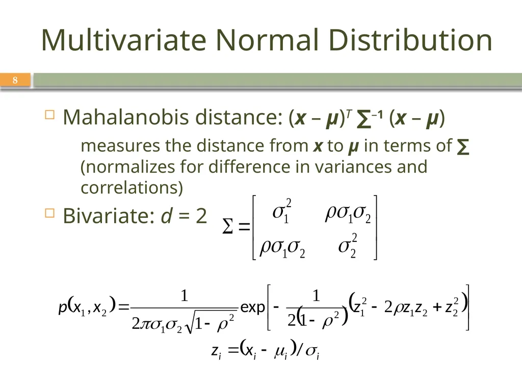
slide8. Multivariate Normal Distribution 8 Mahalanobis distance: (x – μ)T ∑–1 (x – μ)
measures the distance from x to μ in terms of ∑ (normalizes for difference in variances and correlations)
Bivariate: d = 2<br>
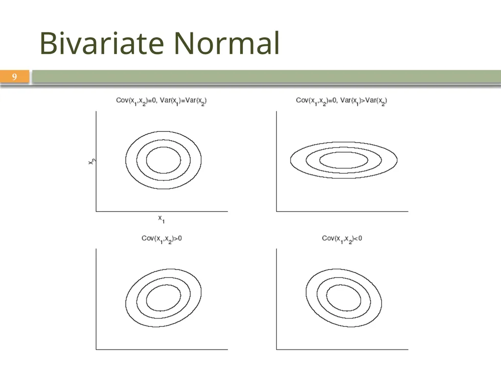
slide9. Bivariate Normal 9<br>
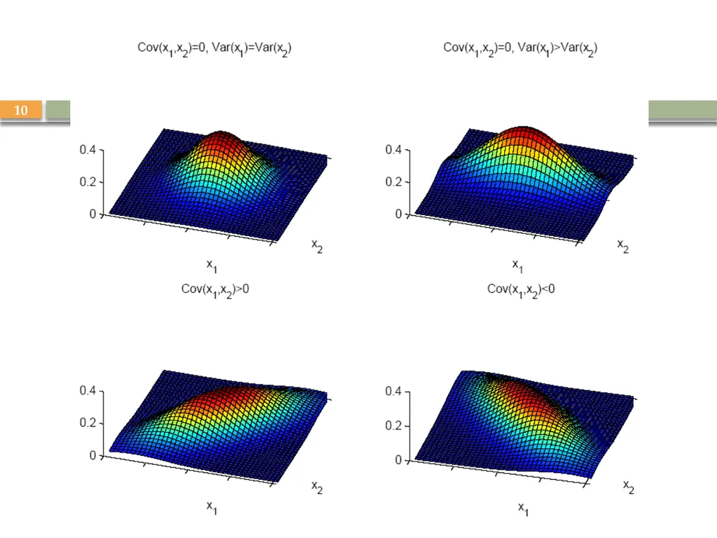
slide10. 10<br>
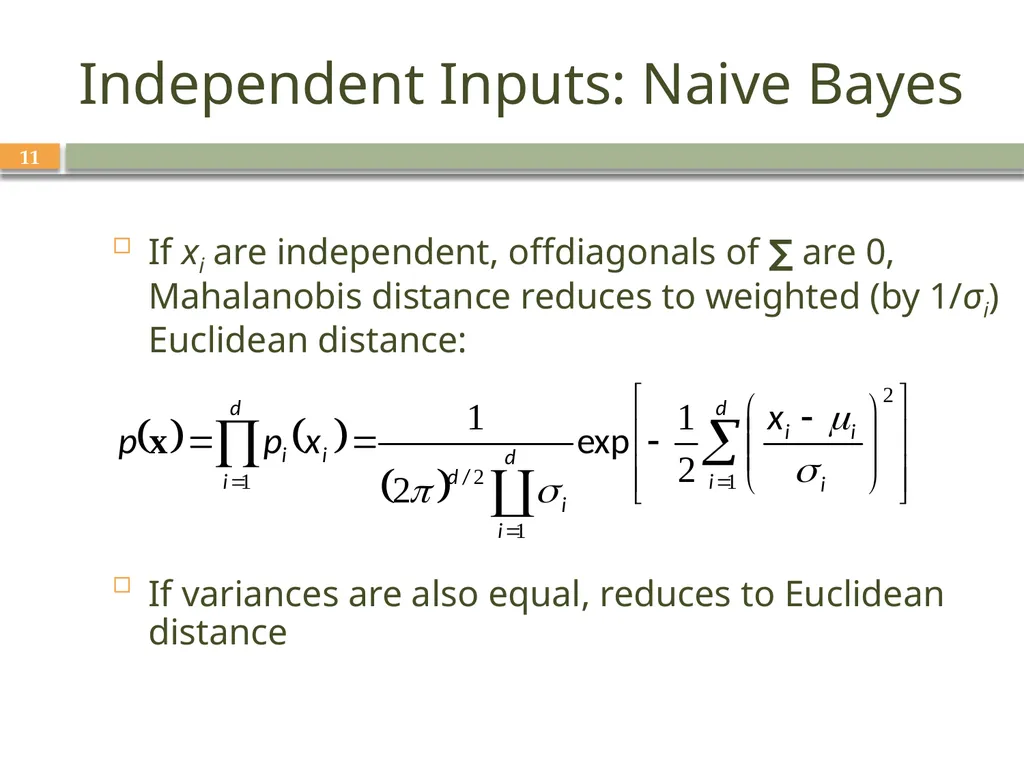
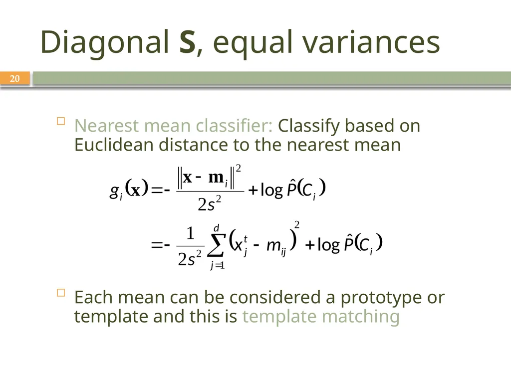
slide11. Independent Inputs: Naive Bayes 11 If xi are independent, offdiagonals of ∑ are 0, Mahalanobis distance reduces to weighted (by 1/σi) Euclidean distance:
If variances are also equal, reduces to Euclidean distance<br>
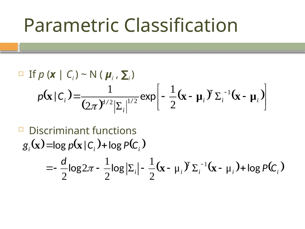
slide12. Parametric Classification If p (x | Ci ) ~ N ( μi , ∑i )
Discriminant functions 12<br>
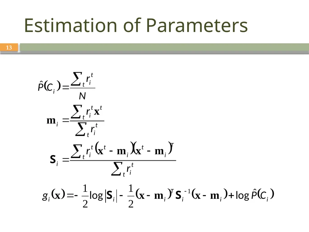
slide13. Estimation of Parameters 13<br>
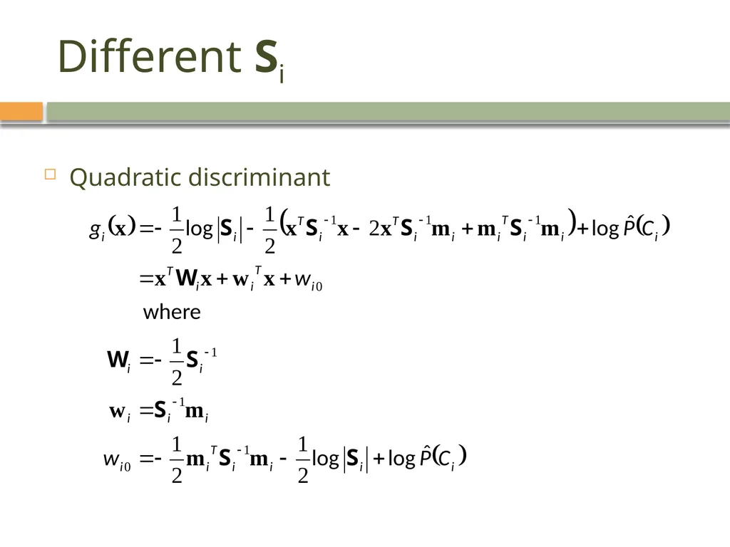
slide14. Different Si Quadratic discriminant 14<br>
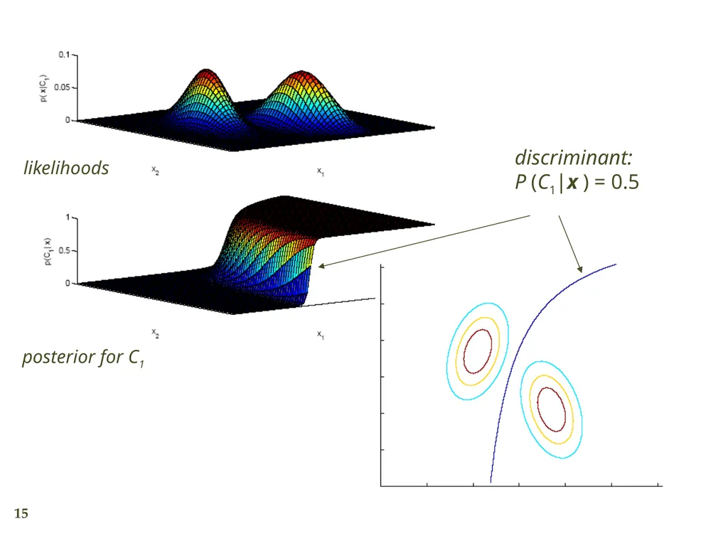
slide15. 15 likelihoods posterior for C1 discriminant:
P (C1|x ) = 0.5<br>
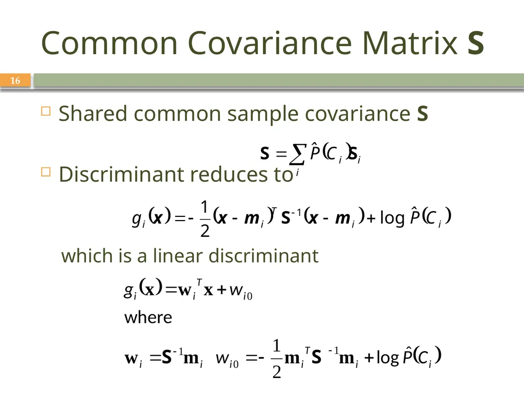
slide16. Common Covariance Matrix S 16 Shared common sample covariance S
Discriminant reduces to
which is a linear discriminant<br>
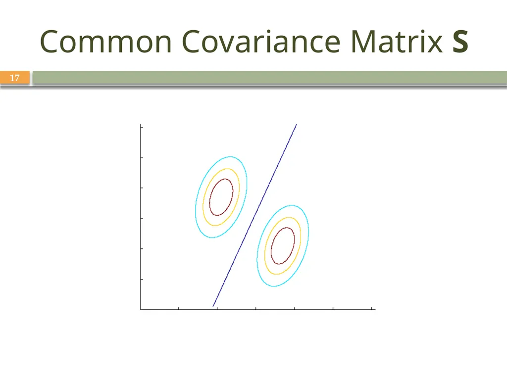
slide17. Common Covariance Matrix S 17<br>
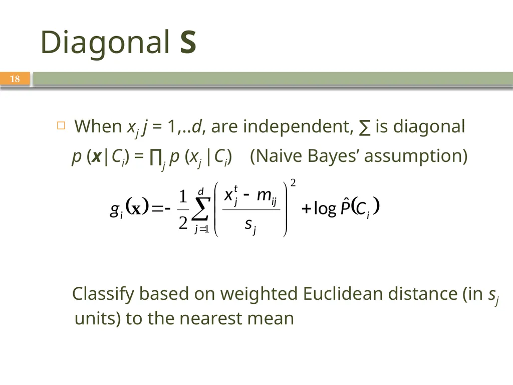
slide18. Diagonal S 18 When xj j = 1,..d, are independent, ∑ is diagonal
p (x|Ci) = ∏j p (xj |Ci) (Naive Bayes’ assumption)
Classify based on weighted Euclidean distance (in sj units) to the nearest mean<br>
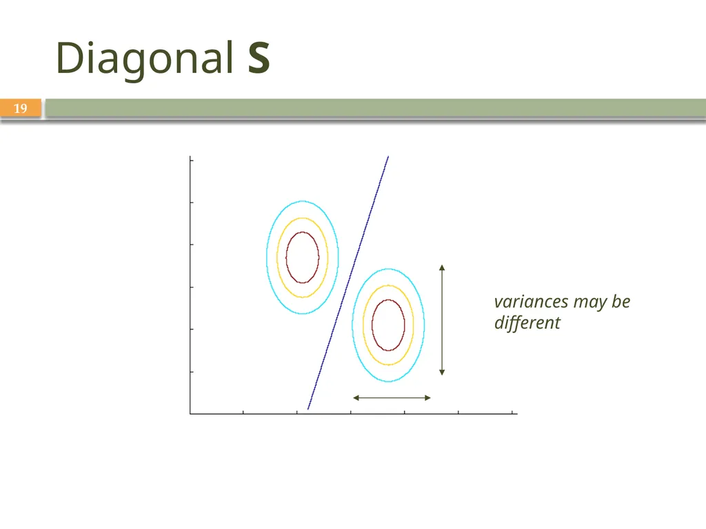
slide19. Diagonal S 19 variances may be
different<br>
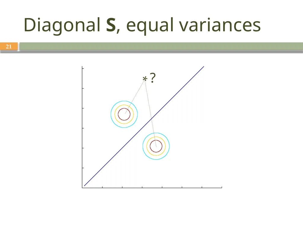
slide20. Diagonal S, equal variances 20 Nearest mean classifier: Classify based on Euclidean distance to the nearest mean
Each mean can be considered a prototype or template and this is template matching<br>
slide21. Diagonal S, equal variances 21 * ?<br>
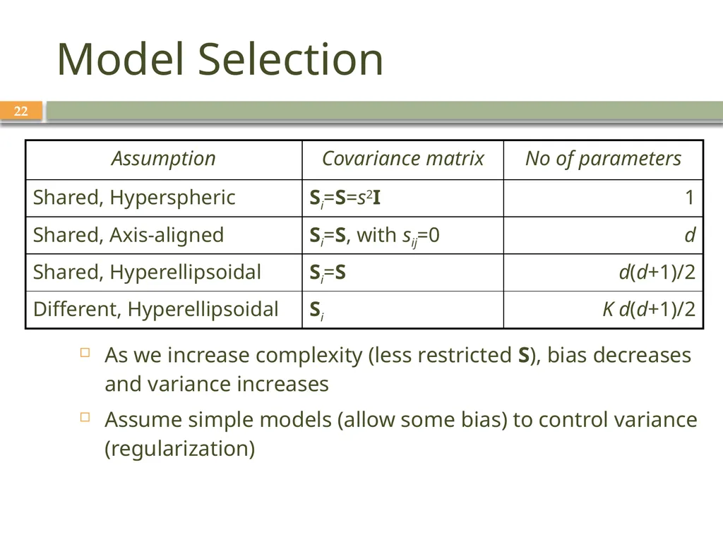
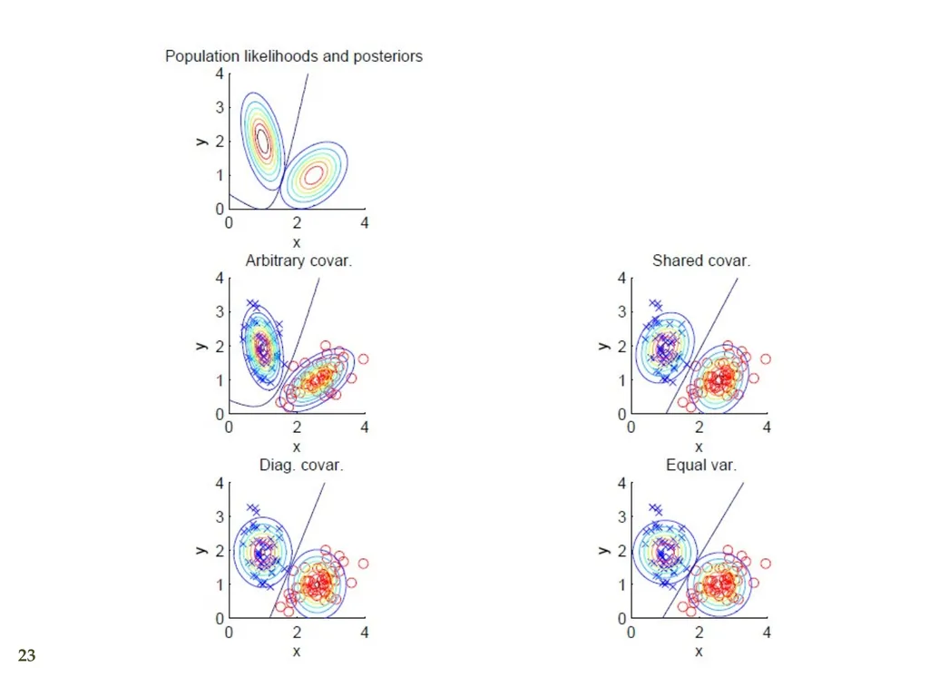
slide22. Model Selection 22 As we increase complexity (less restricted S), bias decreases and variance increases
Assume simple models (allow some bias) to control variance (regularization)<br>
slide23. 23<br>
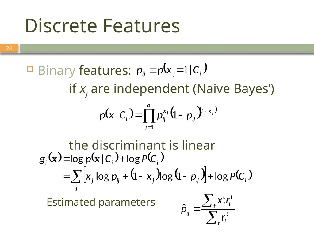
slide24. Discrete Features 24 Binary features:
if xj are independent (Naive Bayes’)
the discriminant is linear Estimated parameters<br>
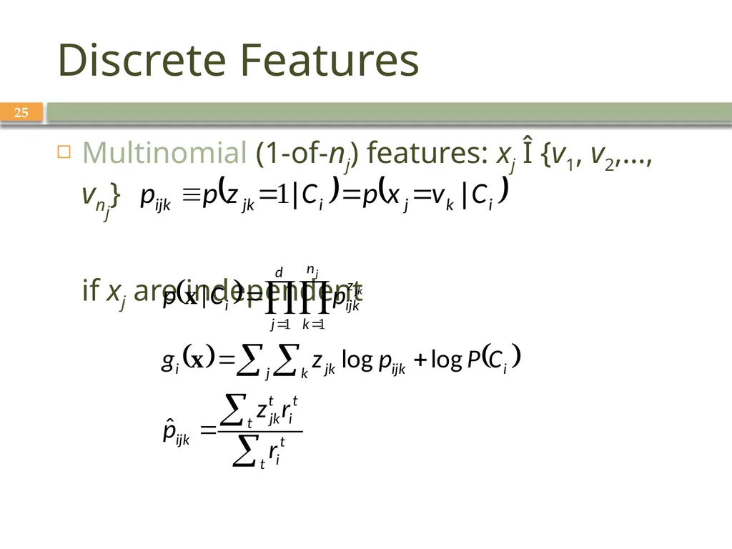
slide25. Discrete Features 25 Multinomial (1-of-nj) features: xj Î {v1, v2,..., vnj}
if xj are independent<br>
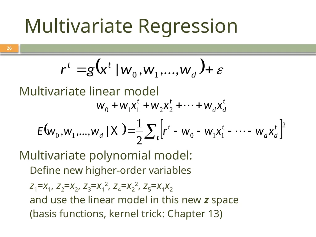
slide26. Multivariate Regression 26 Multivariate linear model
Multivariate polynomial model:
Define new higher-order variables
z1=x1, z2=x2, z3=x12, z4=x22, z5=x1x2
and use the linear model in this new z space
(basis functions, kernel trick: Chapter 13)<br>
© The MIT Press, 2014
alpaydin@boun.edu.tr
http://www.cmpe.boun.edu.tr/~ethem/i2ml3e Lecture Slides for<br>
slide2. CHAPTER 5: Multivariate Methods<br>
slide3. Multivariate Data 3 Multiple measurements (sensors)
d inputs/features/attributes: d-variate
N instances/observations/examples<br>
slide4. Multivariate Parameters 4<br>
slide5. Parameter Estimation 5<br>
slide6. Estimation of Missing Values 6 What to do if certain instances have missing attributes?
Ignore those instances: not a good idea if the sample is small
Use ‘missing’ as an attribute: may give information
Imputation: Fill in the missing value
Mean imputation: Use the most likely value (e.g., mean)
Imputation by regression: Predict based on other attributes<br>
slide7. Multivariate Normal Distribution 7<br>
slide8. Multivariate Normal Distribution 8 Mahalanobis distance: (x – μ)T ∑–1 (x – μ)
measures the distance from x to μ in terms of ∑ (normalizes for difference in variances and correlations)
Bivariate: d = 2<br>
slide9. Bivariate Normal 9<br>
slide10. 10<br>
slide11. Independent Inputs: Naive Bayes 11 If xi are independent, offdiagonals of ∑ are 0, Mahalanobis distance reduces to weighted (by 1/σi) Euclidean distance:
If variances are also equal, reduces to Euclidean distance<br>
slide12. Parametric Classification If p (x | Ci ) ~ N ( μi , ∑i )
Discriminant functions 12<br>
slide13. Estimation of Parameters 13<br>
slide14. Different Si Quadratic discriminant 14<br>
slide15. 15 likelihoods posterior for C1 discriminant:
P (C1|x ) = 0.5<br>
slide16. Common Covariance Matrix S 16 Shared common sample covariance S
Discriminant reduces to
which is a linear discriminant<br>
slide17. Common Covariance Matrix S 17<br>
slide18. Diagonal S 18 When xj j = 1,..d, are independent, ∑ is diagonal
p (x|Ci) = ∏j p (xj |Ci) (Naive Bayes’ assumption)
Classify based on weighted Euclidean distance (in sj units) to the nearest mean<br>
slide19. Diagonal S 19 variances may be
different<br>
slide20. Diagonal S, equal variances 20 Nearest mean classifier: Classify based on Euclidean distance to the nearest mean
Each mean can be considered a prototype or template and this is template matching<br>
slide21. Diagonal S, equal variances 21 * ?<br>
slide22. Model Selection 22 As we increase complexity (less restricted S), bias decreases and variance increases
Assume simple models (allow some bias) to control variance (regularization)<br>
slide23. 23<br>
slide24. Discrete Features 24 Binary features:
if xj are independent (Naive Bayes’)
the discriminant is linear Estimated parameters<br>
slide25. Discrete Features 25 Multinomial (1-of-nj) features: xj Î {v1, v2,..., vnj}
if xj are independent<br>
slide26. Multivariate Regression 26 Multivariate linear model
Multivariate polynomial model:
Define new higher-order variables
z1=x1, z2=x2, z3=x12, z4=x22, z5=x1x2
and use the linear model in this new z space
(basis functions, kernel trick: Chapter 13)<br>