Introductory Statistics and Hypothesis Testing

04

Summary Statistics
Concepts of hypothesis testing
T-tests
Confidence intervals
Correlation and Regression
Choosing the right test
What is a non-parametric test?
Statistics scenarios
Top tips
ANOVA (if time) www.statstutor.ac.uk Content

05

Lots of maths!!!

Students coming to statistics support usually want help with using SPSS, choosing the right analysis and interpreting output

They often find maths scary and so you need to think of ways of explaining without the maths www.statstutor.ac.uk What we won’t cover

06

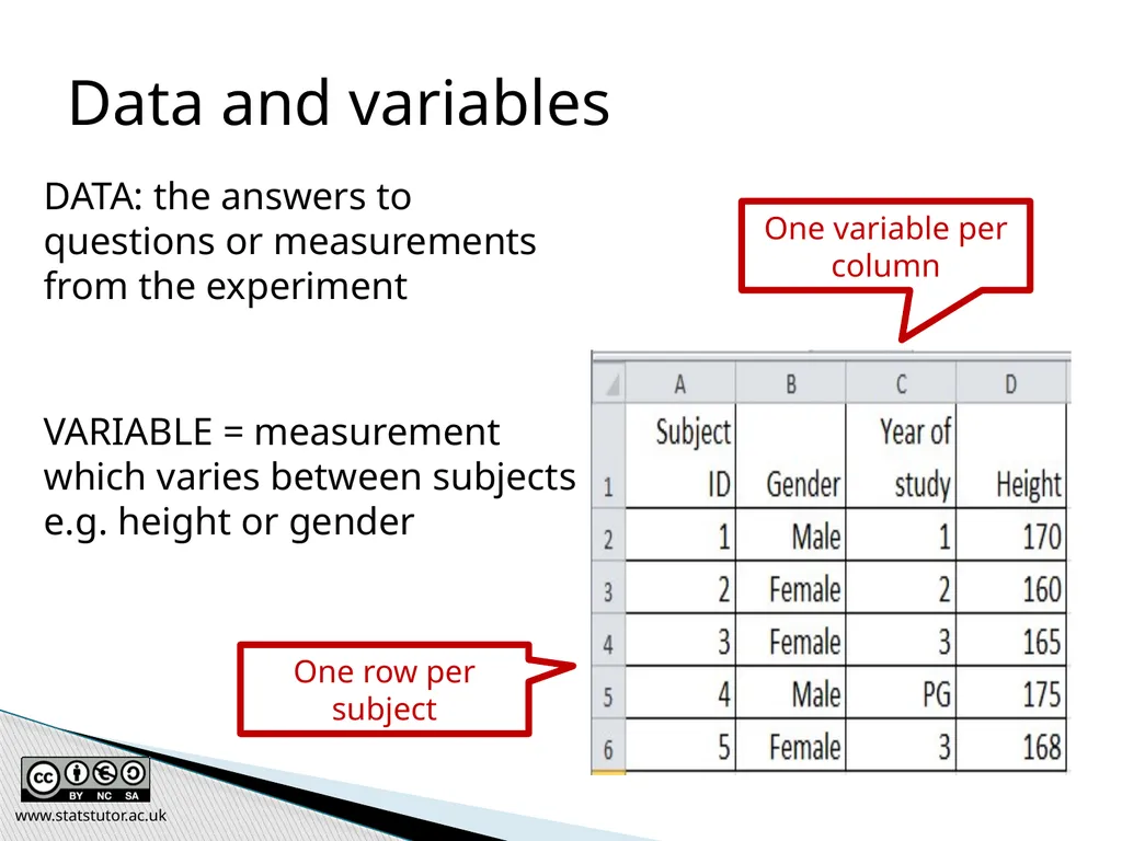
DATA: the answers to questions or measurements from the experiment

VARIABLE = measurement which varies between subjects e.g. height or gender Data and variables One row per subject One variable per column www.statstutor.ac.uk

07

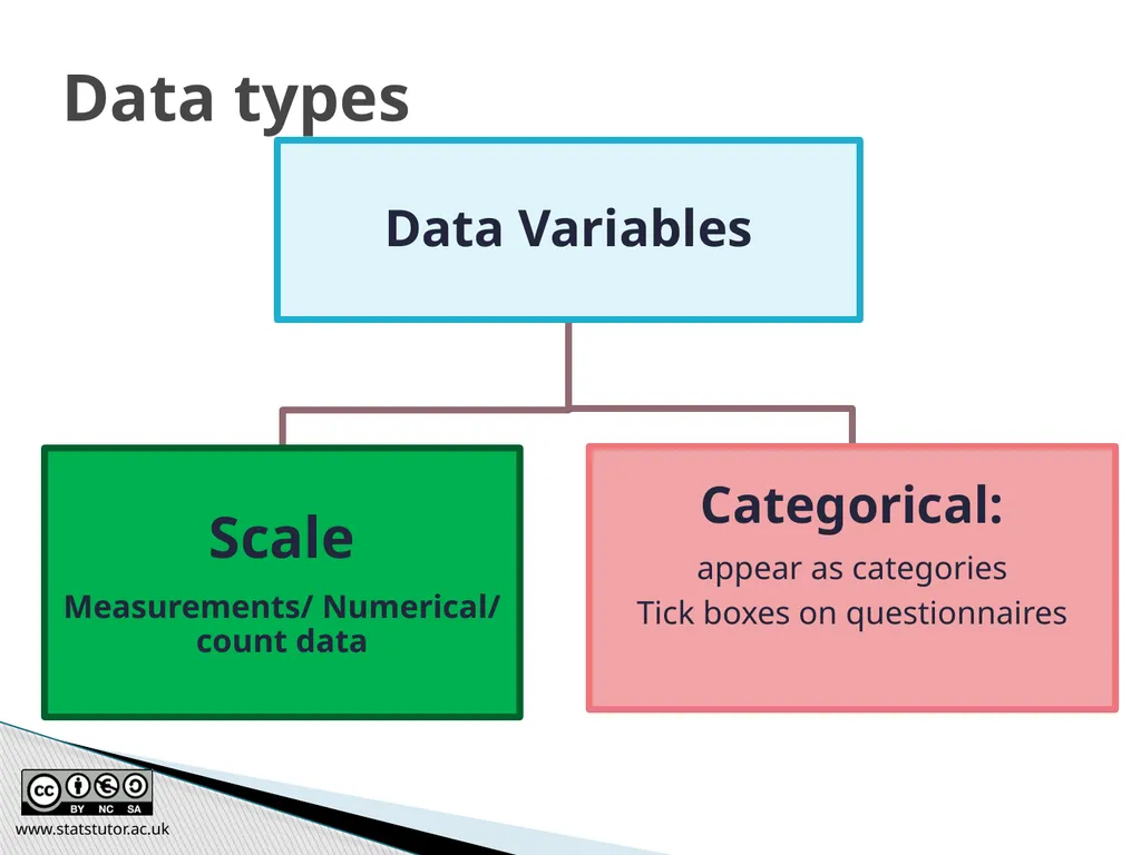
Data types www.statstutor.ac.uk

08

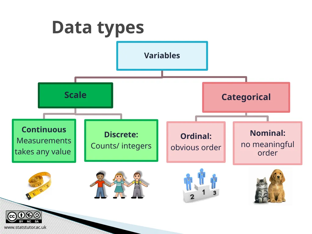
www.statstutor.ac.uk Data types

09

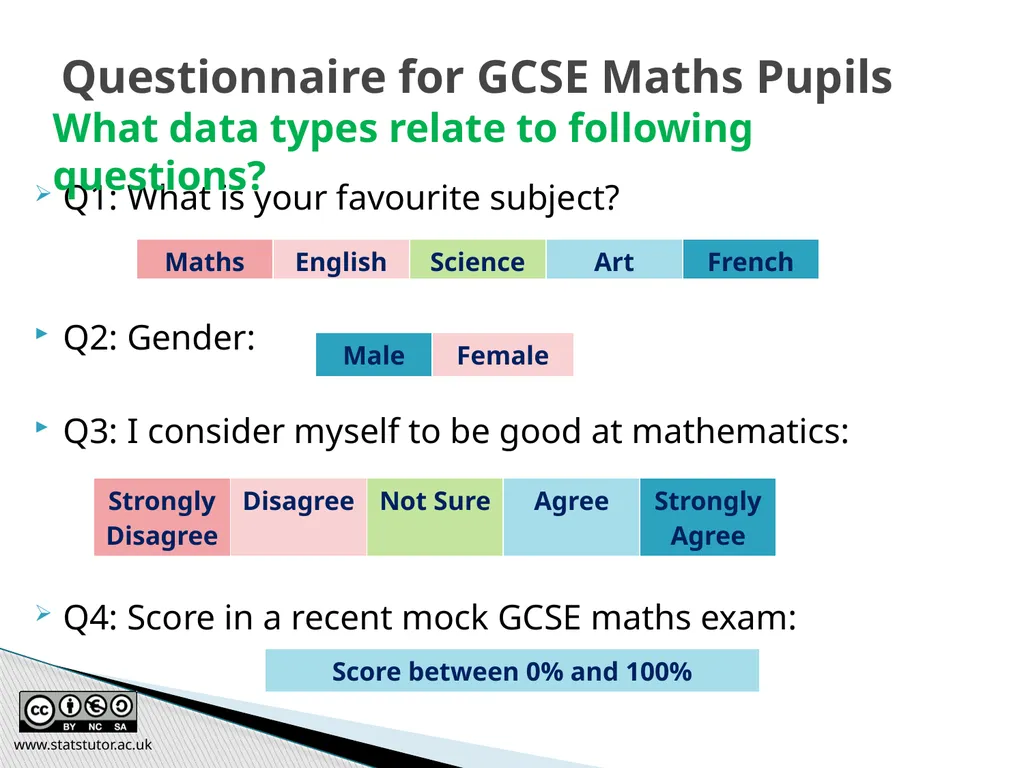
Q1: What is your favourite subject?

Q2: Gender:

Q3: I consider myself to be good at mathematics:

Q4: Score in a recent mock GCSE maths exam: Questionnaire for GCSE Maths Pupils What data types relate to following questions? www.statstutor.ac.uk

10

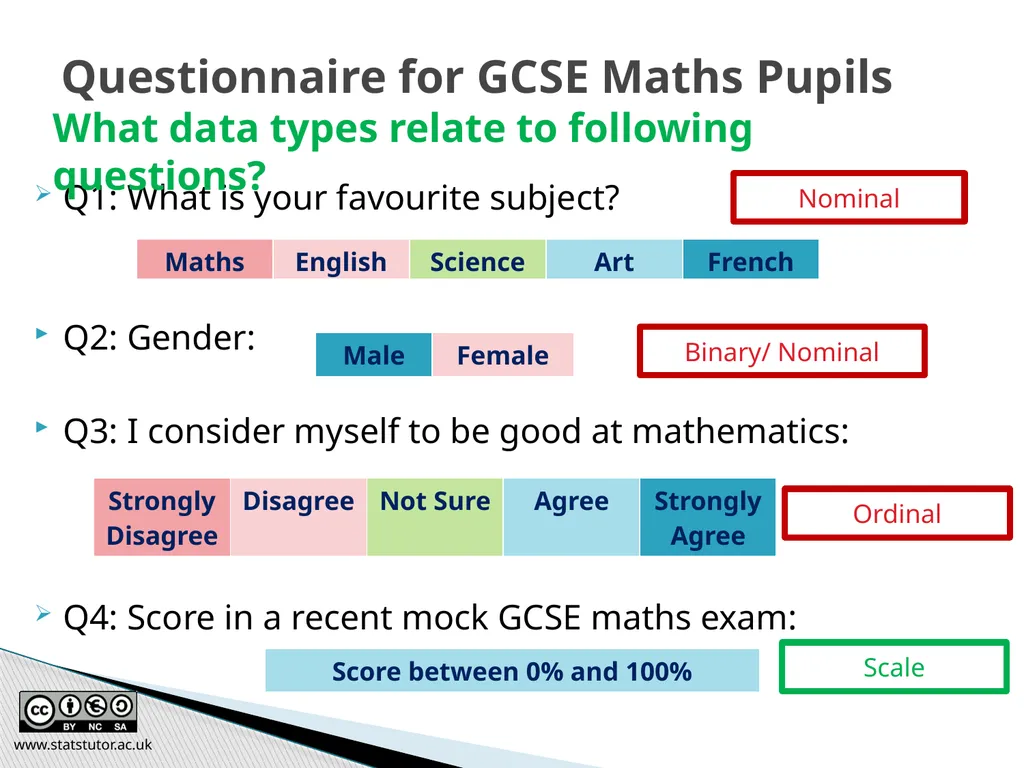
Q1: What is your favourite subject?

Q2: Gender:

Q3: I consider myself to be good at mathematics:

Q4: Score in a recent mock GCSE maths exam: Questionnaire for GCSE Maths Pupils What data types relate to following questions? www.statstutor.ac.uk Nominal Binary/ Nominal Ordinal Scale

11

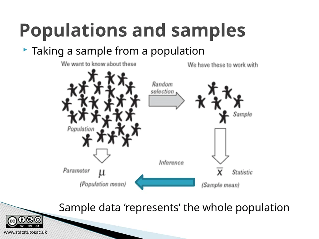
Taking a sample from a population Populations and samples www.statstutor.ac.uk Sample data ‘represents’ the whole population

12

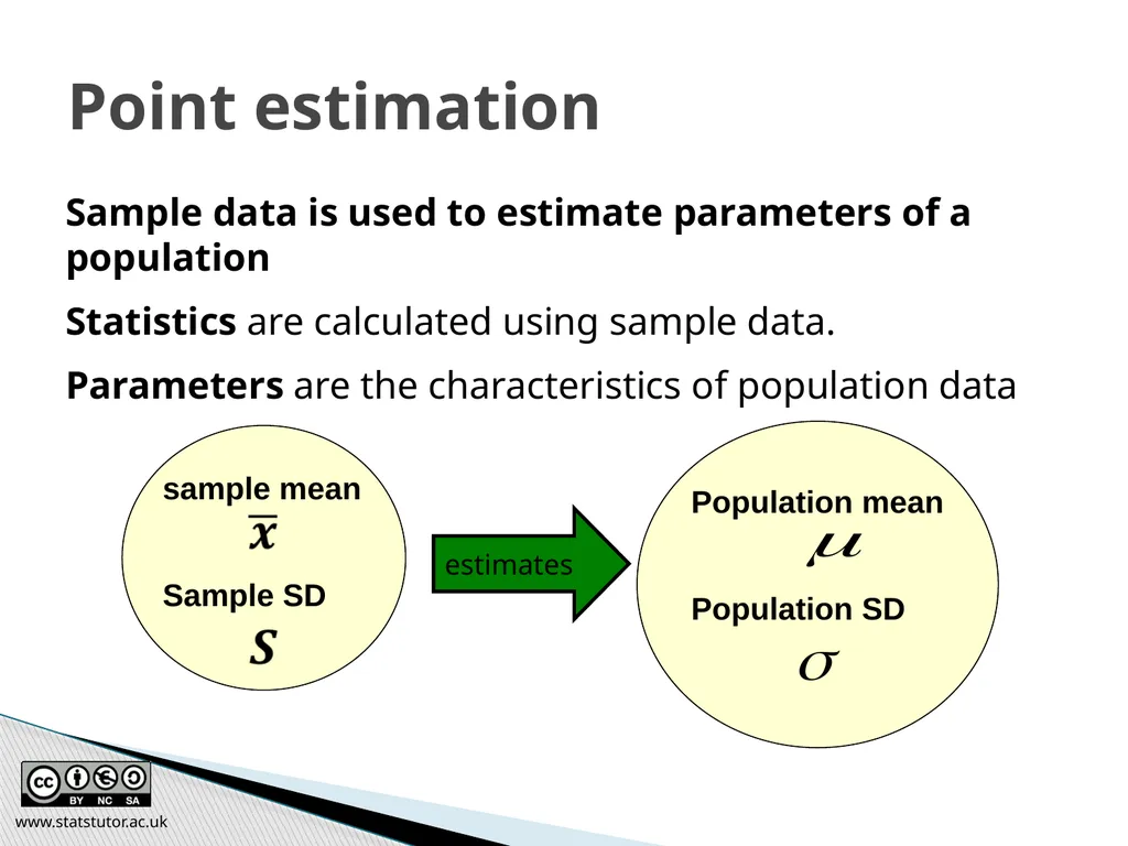
Population mean

Population SD www.statstutor.ac.uk Point estimation sample mean

Sample SD Sample data is used to estimate parameters of a population
Statistics are calculated using sample data.
Parameters are the characteristics of population data estimates

13

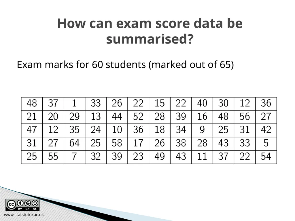
Exam marks for 60 students (marked out of 65)

mean = 30.3 sd = 14.46 www.statstutor.ac.uk How can exam score data be summarised?

14

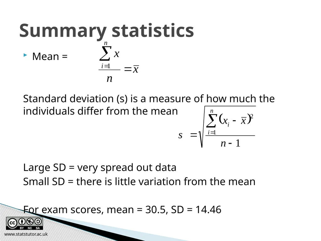
Mean =

Standard deviation (s) is a measure of how much the individuals differ from the mean

Large SD = very spread out data
Small SD = there is little variation from the mean

For exam scores, mean = 30.5, SD = 14.46 Summary statistics www.statstutor.ac.uk

15

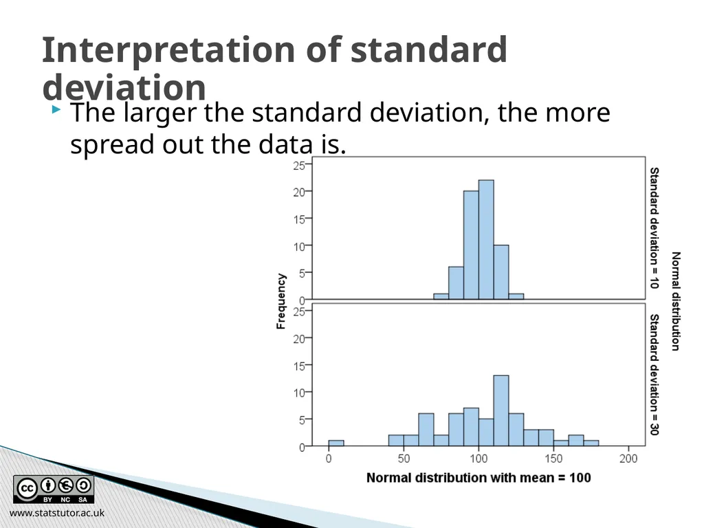
The larger the standard deviation, the more spread out the data is. Interpretation of standard deviation www.statstutor.ac.uk

16

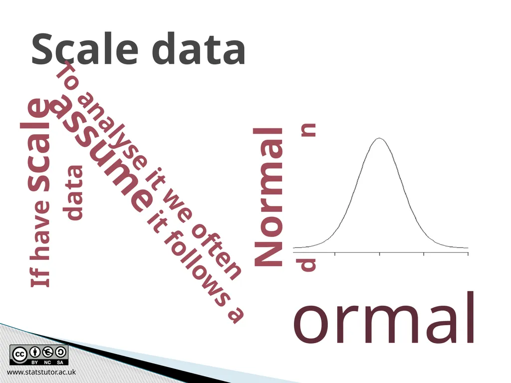
www.statstutor.ac.uk Scale data If have scale data assume it follows a Normal distribution To analyse it we often ormal

17

How could you explain to a student what we mean by data being assumed to follow a Normal Distribution? www.statstutor.ac.uk Discussion

18

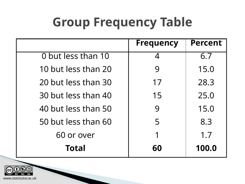
www.statstutor.ac.uk Group Frequency Table

19

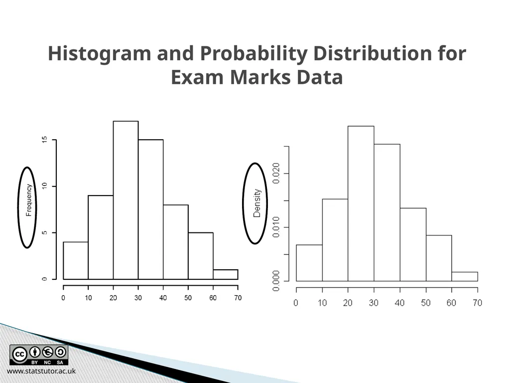
www.statstutor.ac.uk Histogram and Probability Distribution forExam Marks Data

20

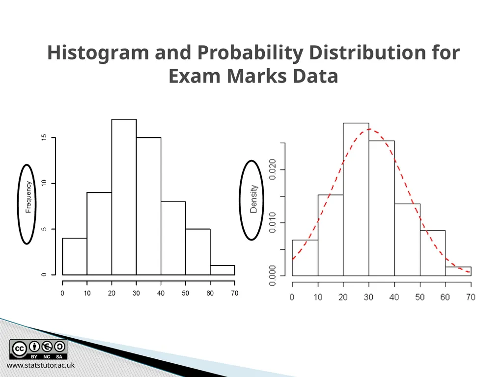
www.statstutor.ac.uk Histogram and Probability Distribution forExam Marks Data

21

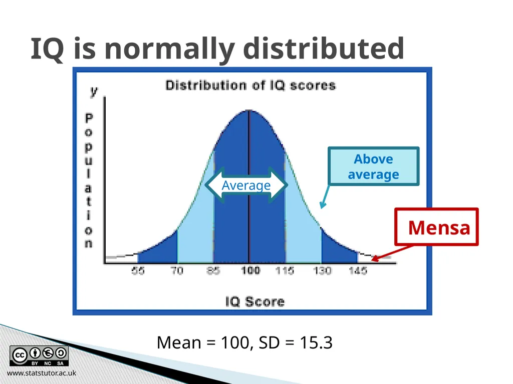
IQ is normally distributed Above average Average Mensa Mean = 100, SD = 15.3 www.statstutor.ac.uk

22

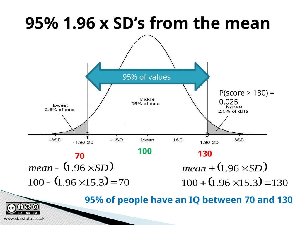
95% of values 95% 1.96 x SD’s from the mean 70 130 100 P(score > 130) = 0.025 95% of people have an IQ between 70 and 130 www.statstutor.ac.uk

23

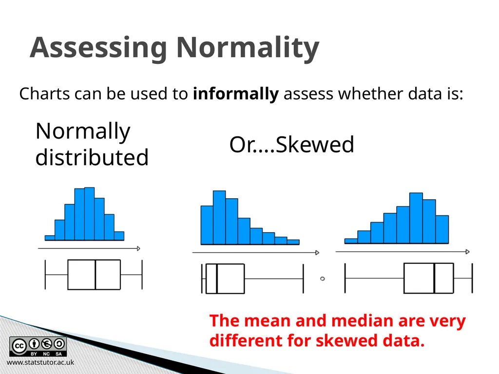
Charts can be used to informally assess whether data is: www.statstutor.ac.uk Assessing Normality Normally
distributed Or….Skewed The mean and median are very different for skewed data.

24

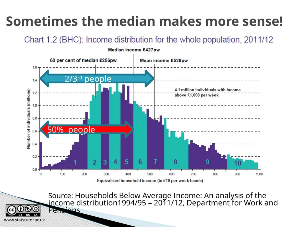
Discussion Is the following statement:

“2 out of 3 people earn less than the average income”

True
False
Don’t know www.statstutor.ac.uk

25

Source: Households Below Average Income: An analysis of the income distribution1994/95 – 2011/12, Department for Work and Pensions www.statstutor.ac.uk Sometimes the median makes more sense! 2/3rd people 50% people

26

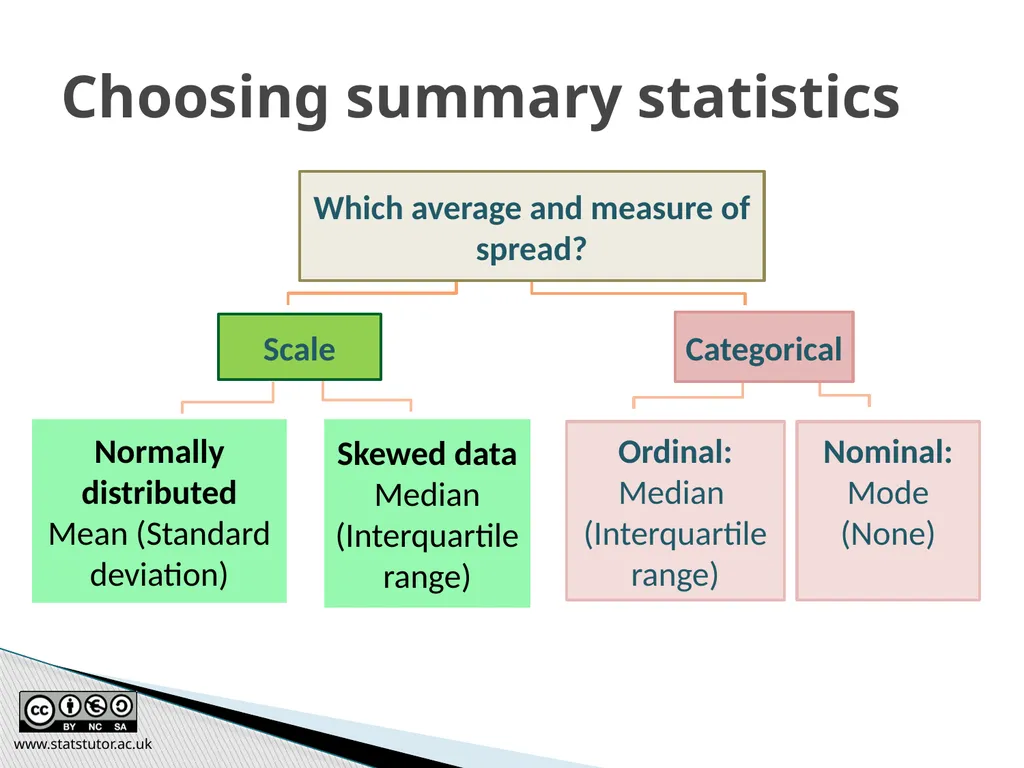
www.statstutor.ac.uk Choosing summary statistics

27

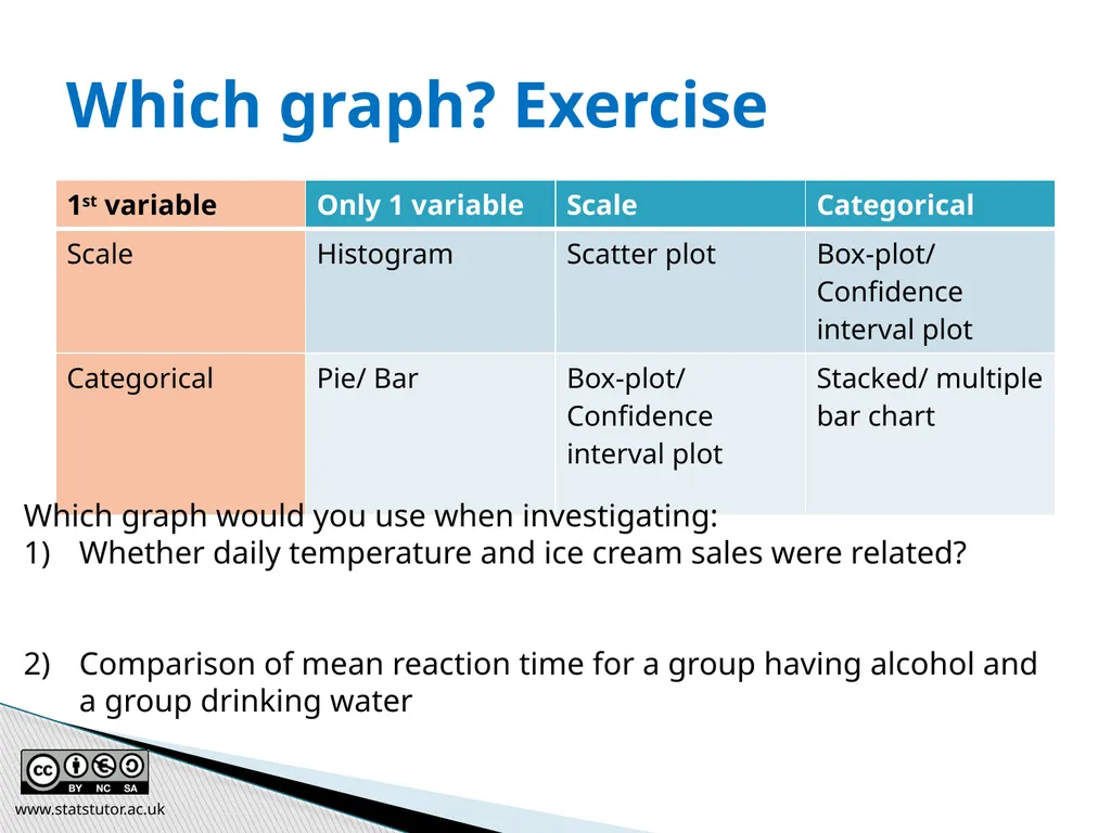
Which graph? Exercise Which graph would you use when investigating:
Whether daily temperature and ice cream sales were related?

Comparison of mean reaction time for a group having alcohol and a group drinking water www.statstutor.ac.uk

28

Summary statistics for cost of Titanic ticket by survival

Is there a big difference in average ticket price by group?

Which group has data which is more spread out?

Is the data skewed?

Is the mean or median a better summary measure? Exercise: Ticket cost comparison www.statstutor.ac.uk www.statstutor.ac.uk

29

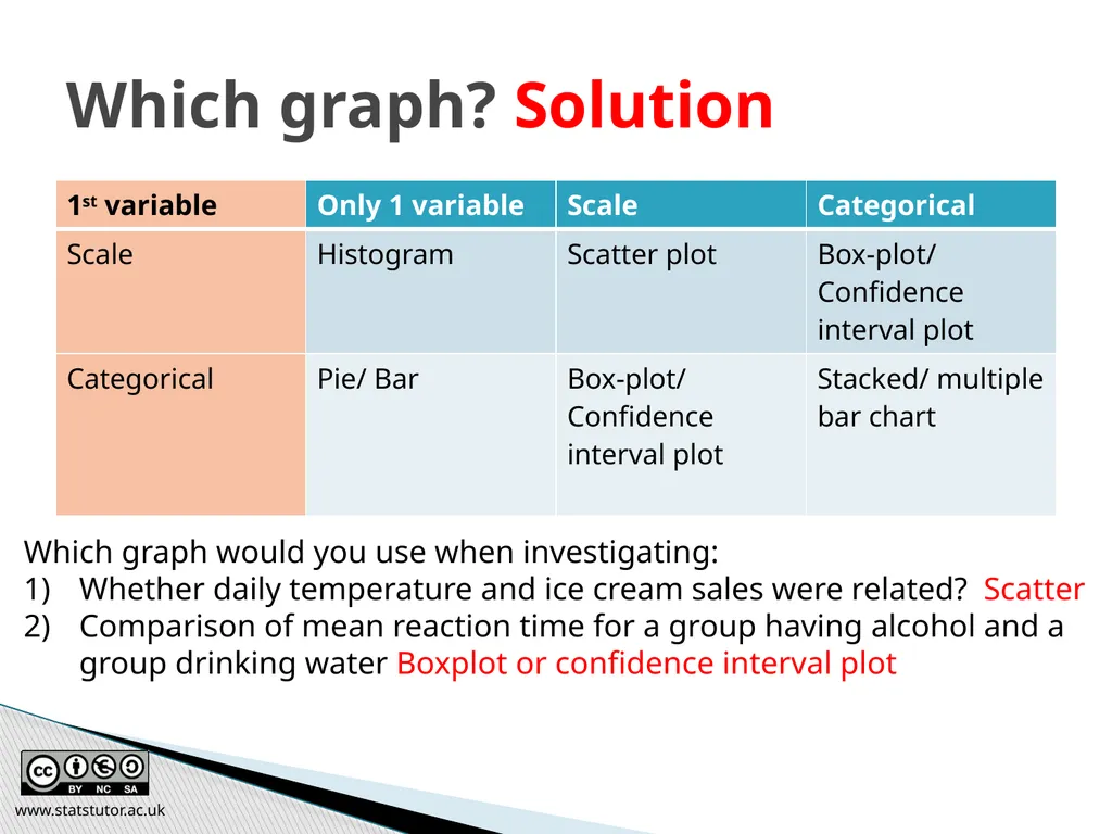
Which graph? Solution Which graph would you use when investigating:
Whether daily temperature and ice cream sales were related? Scatter
Comparison of mean reaction time for a group having alcohol and a group drinking water Boxplot or confidence interval plot www.statstutor.ac.uk

30

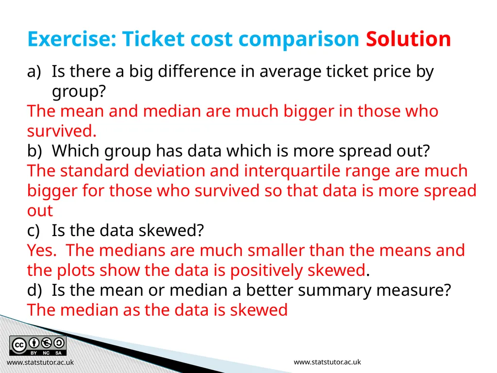
Is there a big difference in average ticket price by group?
The mean and median are much bigger in those who survived.
Which group has data which is more spread out?
The standard deviation and interquartile range are much bigger for those who survived so that data is more spread out
Is the data skewed?
Yes. The medians are much smaller than the means and the plots show the data is positively skewed.
Is the mean or median a better summary measure?
The median as the data is skewed Exercise: Ticket cost comparison Solution www.statstutor.ac.uk www.statstutor.ac.uk

31

Hypothesis Testing www.statstutor.ac.uk Ellen Marshall / Alun Owen
University of Sheffield / University of Worcester Reviewer: Ruth Fairclough
University of Wolverhampton community project
encouraging academics to share statistics support resources
All stcp resources are released under a Creative Commons licence

32

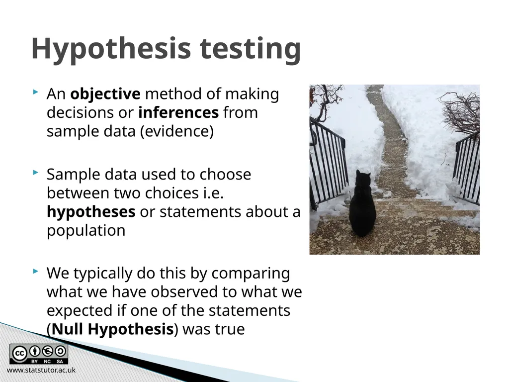
An objective method of making decisions or inferences from sample data (evidence)

Sample data used to choose between two choices i.e. hypotheses or statements about a population

We typically do this by comparing what we have observed to what we expected if one of the statements (Null Hypothesis) was true www.statstutor.ac.uk Hypothesis testing

33

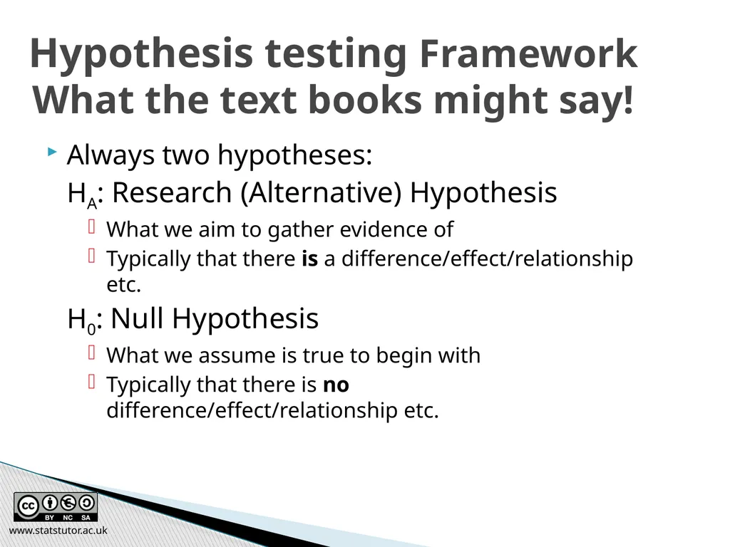
www.statstutor.ac.uk Hypothesis testing FrameworkWhat the text books might say! Always two hypotheses:
HA: Research (Alternative) Hypothesis
What we aim to gather evidence of
Typically that there is a difference/effect/relationship etc.
H0: Null Hypothesis
What we assume is true to begin with
Typically that there is no difference/effect/relationship etc.

34

How could you help a student understand what hypothesis testing is and why they need to use it? www.statstutor.ac.uk Discussion

35

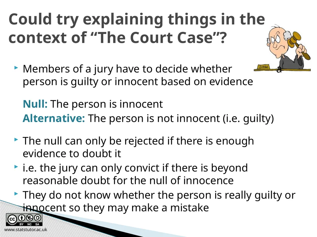
Members of a jury have to decide whether a person is guilty or innocent based on evidence

Null: The person is innocent
Alternative: The person is not innocent (i.e. guilty)

The null can only be rejected if there is enough evidence to doubt it
i.e. the jury can only convict if there is beyond reasonable doubt for the null of innocence
They do not know whether the person is really guilty or innocent so they may make a mistake www.statstutor.ac.uk Could try explaining things in the context of “The Court Case”?

36

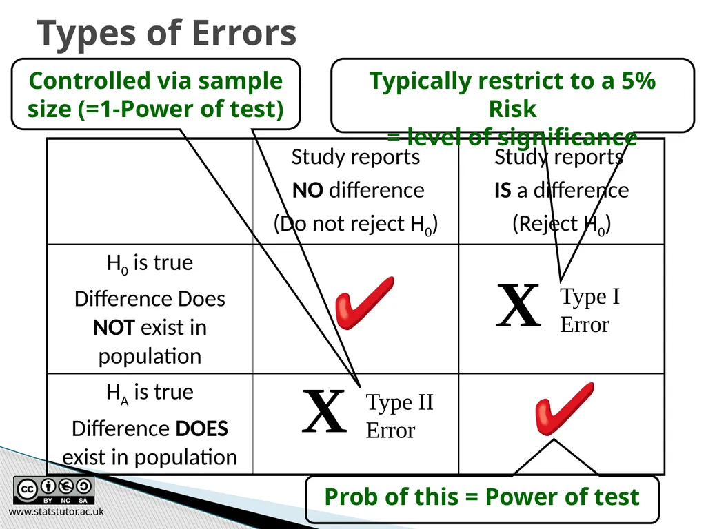
Types of Errors www.statstutor.ac.uk Controlled via sample size (=1-Power of test) Typically restrict to a 5% Risk
= level of significance Prob of this = Power of test Type I Error X Type II Error X

37

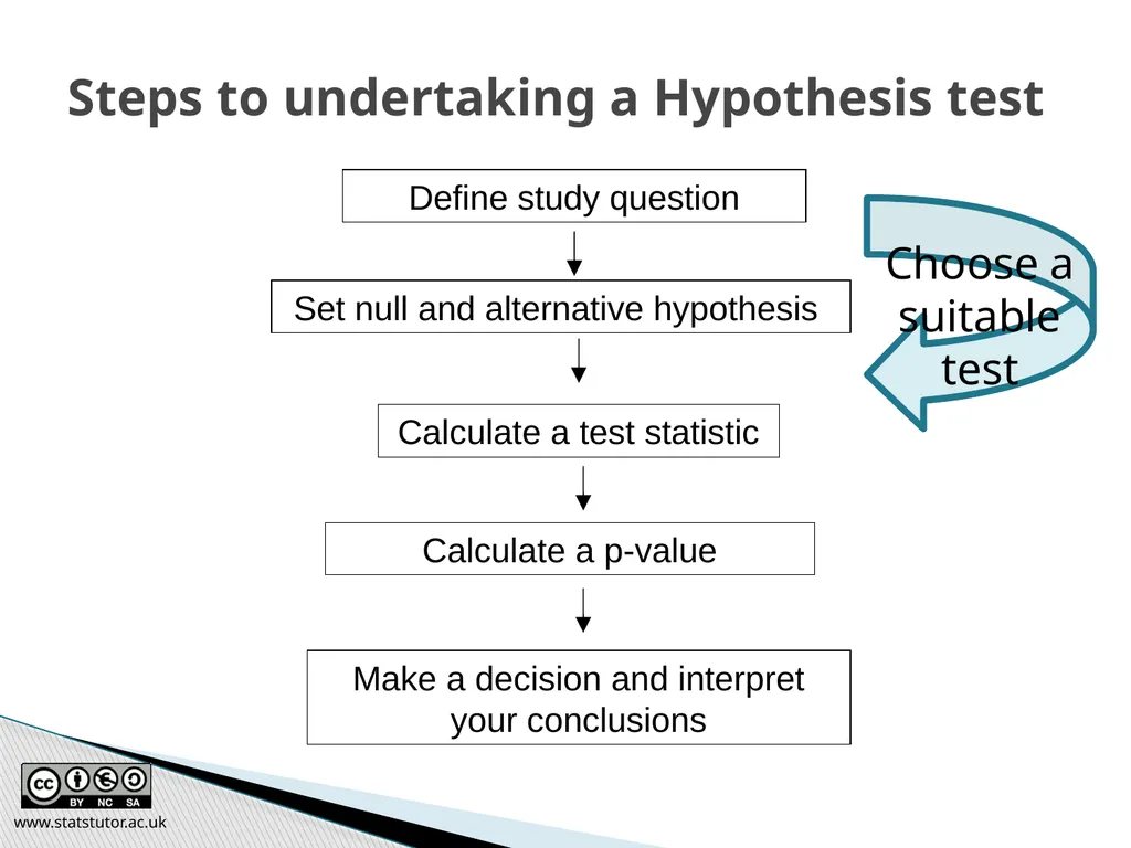
Steps to undertaking a Hypothesis test www.statstutor.ac.uk Choose a suitable test

38

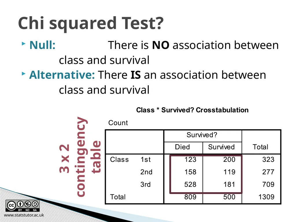
The ship Titanic sank in 1912 with the loss of most of its passengers
809 of the 1,309 passengers and crew died
= 61.8%
Research question: Did class (of travel) affect survival? www.statstutor.ac.uk Example: Titanic

39

Null: There is NO association between
class and survival
Alternative: There IS an association between
class and survival www.statstutor.ac.uk Chi squared Test? 3 x 2
contingency table

40

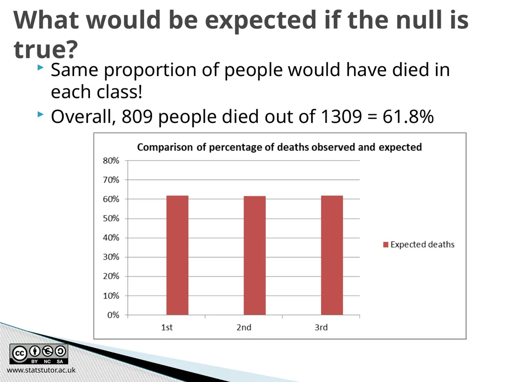
Same proportion of people would have died in each class!
Overall, 809 people died out of 1309 = 61.8% www.statstutor.ac.uk What would be expected if the null is true?

41

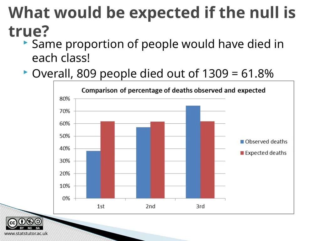
Same proportion of people would have died in each class!
Overall, 809 people died out of 1309 = 61.8% www.statstutor.ac.uk What would be expected if the null is true?

42

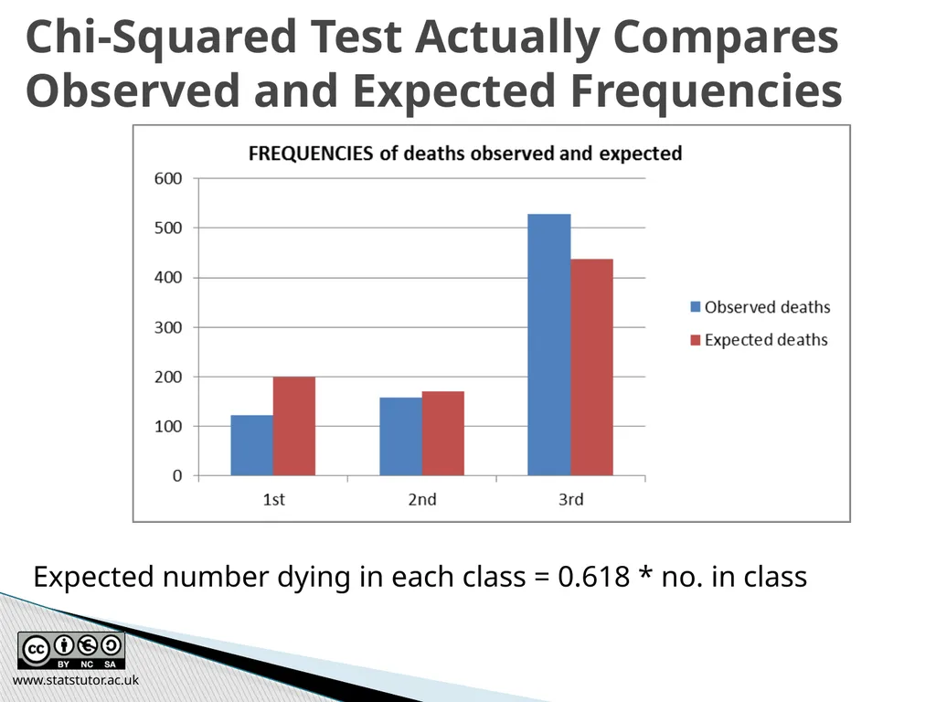
www.statstutor.ac.uk Chi-Squared Test Actually Compares Observed and Expected Frequencies Expected number dying in each class = 0.618 * no. in class

43

The chi-squared test is used when we want to see if two categorical variables are related
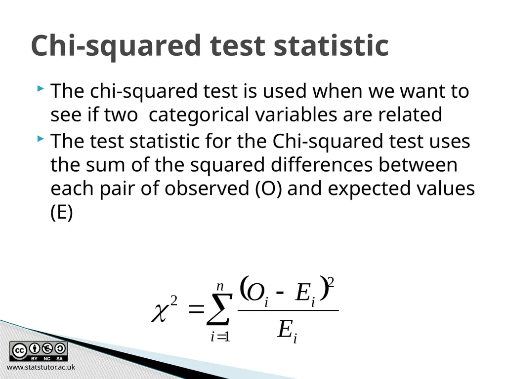
The test statistic for the Chi-squared test uses the sum of the squared differences between each pair of observed (O) and expected values (E) www.statstutor.ac.uk Chi-squared test statistic

44

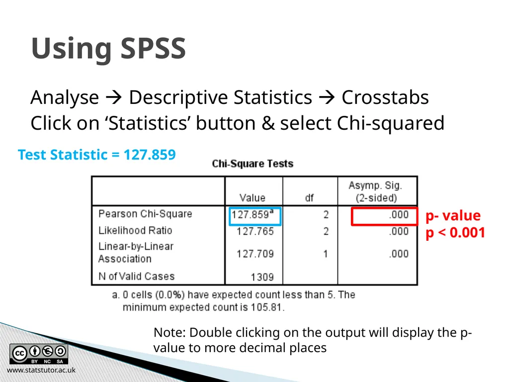
Analyse  Descriptive Statistics  Crosstabs
Click on ‘Statistics’ button & select Chi-squared www.statstutor.ac.uk Using SPSS p- value
p < 0.001 Test Statistic = 127.859 Note: Double clicking on the output will display the p-value to more decimal places

45

We can use statistical software to undertake a hypothesis test e.g. SPSS
One part of the output is the p-value (P)

If P < 0.05 reject H0 => Evidence of HA being true (i.e. IS association)

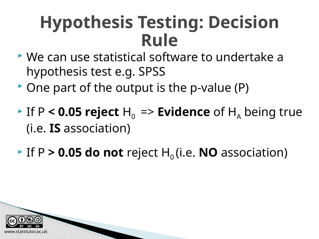
If P > 0.05 do not reject H0 (i.e. NO association) www.statstutor.ac.uk Hypothesis Testing: Decision Rule

46

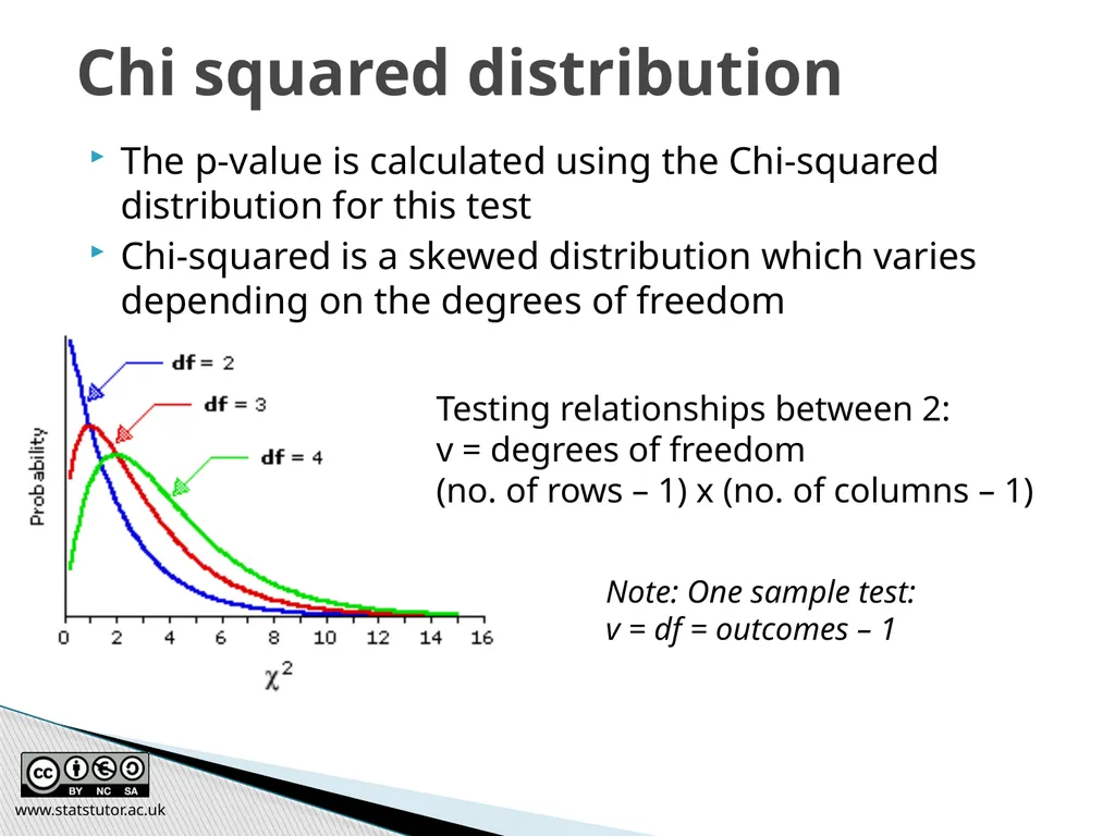
The p-value is calculated using the Chi-squared distribution for this test
Chi-squared is a skewed distribution which varies depending on the degrees of freedom www.statstutor.ac.uk Chi squared distribution Testing relationships between 2:
v = degrees of freedom
(no. of rows – 1) x (no. of columns – 1) Note: One sample test:
v = df = outcomes – 1

47

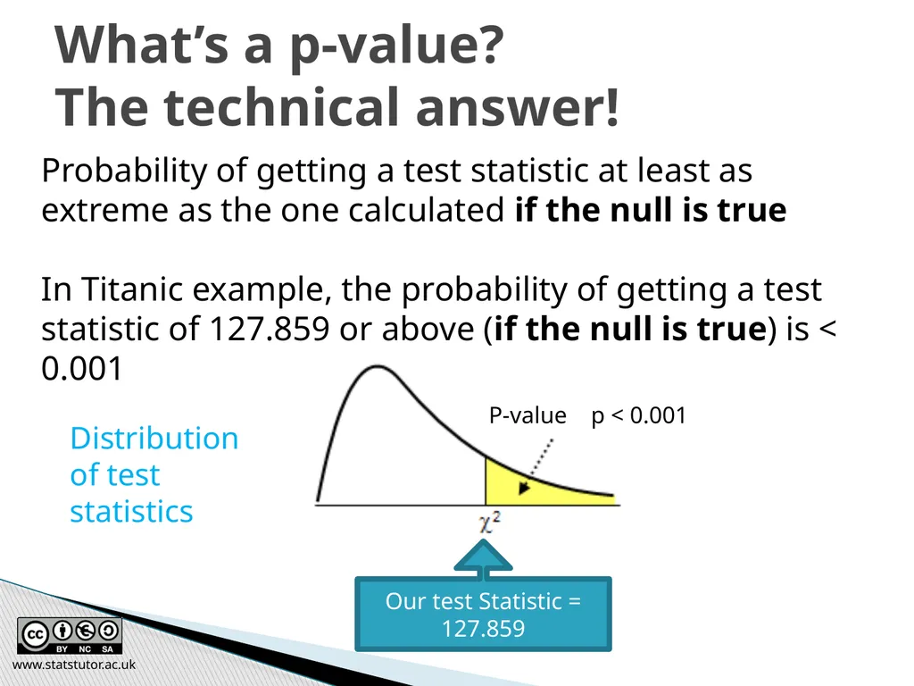
www.statstutor.ac.uk What’s a p-value?The technical answer! Probability of getting a test statistic at least as extreme as the one calculated if the null is true

In Titanic example, the probability of getting a test statistic of 127.859 or above (if the null is true) is < 0.001 Our test Statistic = 127.859 P-value p < 0.001 Distribution of test statistics

48

www.statstutor.ac.uk Interpretation Test Statistic = 127.859 P-value
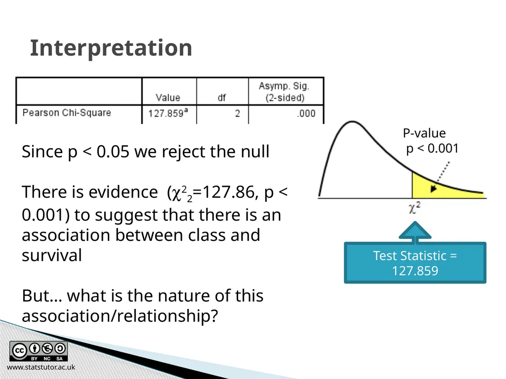
p < 0.001 Since p < 0.05 we reject the null

There is evidence (c22=127.86, p < 0.001) to suggest that there is an association between class and survival

But… what is the nature of this association/relationship?

49

Were ‘wealthy’ people more likely to survive on board the Titanic?

Option 1:
Choose the right percentages from the next slide to investigate
Fill in the stacked bar chart with the chosen %’s
Write a summary to go with the chart Titanic exercise www.statstutor.ac.uk

50

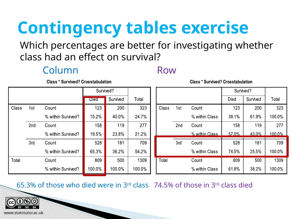
Which percentages are better for investigating whether class had an effect on survival?
Column Row

65.3% of those who died were in 3rd class 74.5% of those in 3rd class died Contingency tables exercise www.statstutor.ac.uk

51

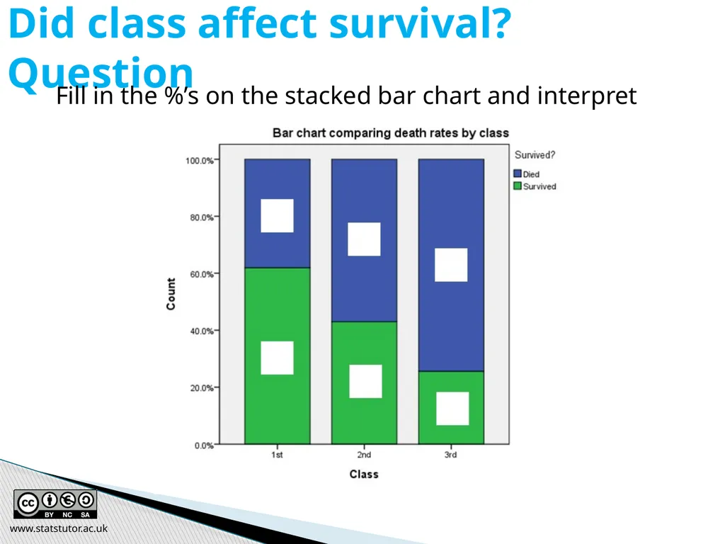
Did class affect survival? Question Fill in the %’s on the stacked bar chart and interpret www.statstutor.ac.uk

52

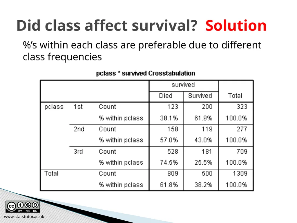
Did class affect survival? Solution %’s within each class are preferable due to different class frequencies www.statstutor.ac.uk

53

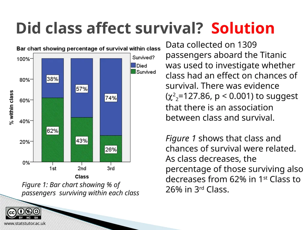
Data collected on 1309 passengers aboard the Titanic was used to investigate whether class had an effect on chances of survival. There was evidence (c22=127.86, p < 0.001) to suggest that there is an association between class and survival.

Figure 1 shows that class and chances of survival were related. As class decreases, the percentage of those surviving also decreases from 62% in 1st Class to 26% in 3rd Class. Figure 1: Bar chart showing % of passengers surviving within each class Did class affect survival? Solution www.statstutor.ac.uk

54

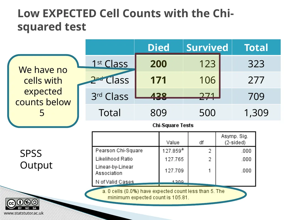
www.statstutor.ac.uk Low EXPECTED Cell Counts with the Chi-squared test SPSS Output We have no cells with expected counts below 5

55

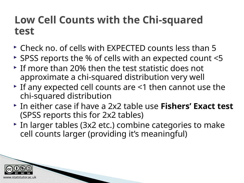
Check no. of cells with EXPECTED counts less than 5
SPSS reports the % of cells with an expected count <5
If more than 20% then the test statistic does not approximate a chi-squared distribution very well
If any expected cell counts are <1 then cannot use the chi-squared distribution
In either case if have a 2x2 table use Fishers’ Exact test (SPSS reports this for 2x2 tables)
In larger tables (3x2 etc.) combine categories to make cell counts larger (providing it’s meaningful) www.statstutor.ac.uk Low Cell Counts with the Chi-squared test

56

Comparing means www.statstutor.ac.uk Ellen Marshall / Alun Owen
University of Sheffield / University of Worcester Reviewer: Ruth Fairclough
University of Wolverhampton community project
encouraging academics to share statistics support resources
All stcp resources are released under a Creative Commons licence

57

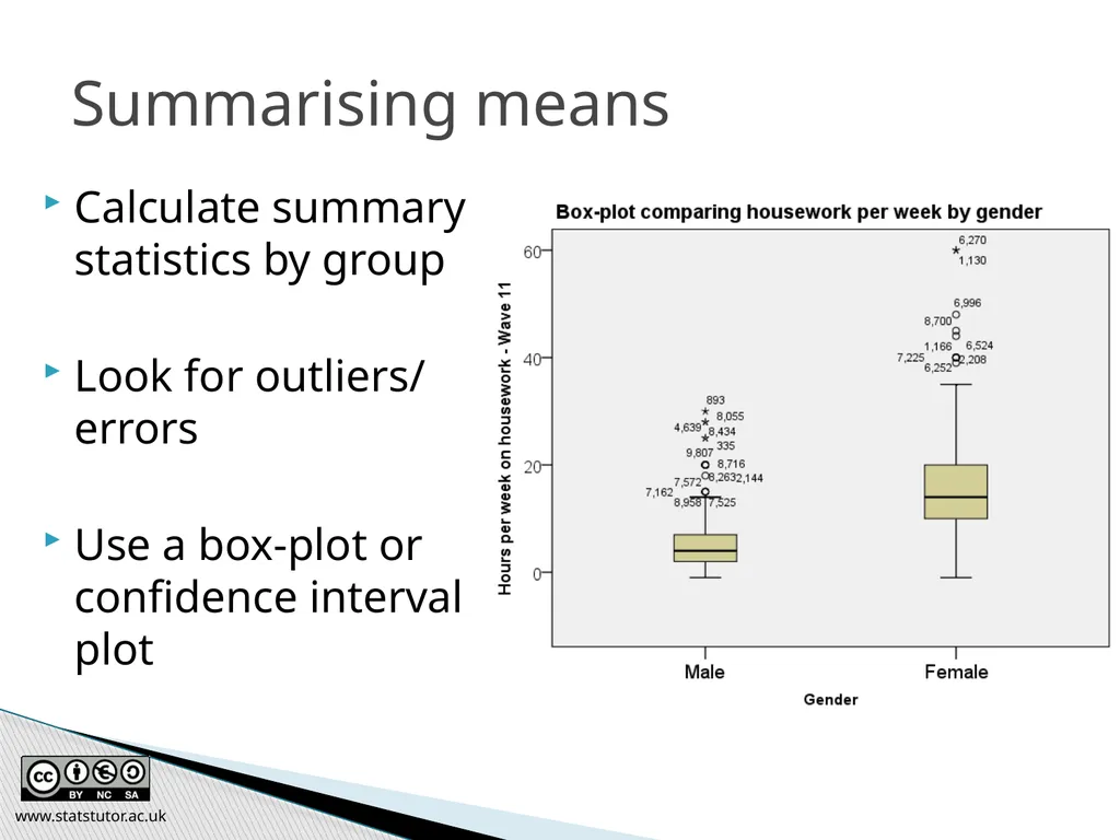
Summarising means Calculate summary statistics by group

Look for outliers/ errors

Use a box-plot or confidence interval plot www.statstutor.ac.uk

58

www.statstutor.ac.uk T-testsPaired or Independent (Unpaired) Data? T-tests are used to compare two population means
Paired data: same individuals studied at two different times or under two conditions PAIRED T-TEST
Independent: data collected from two separate groups INDEPENDENT SAMPLES T-TEST

59

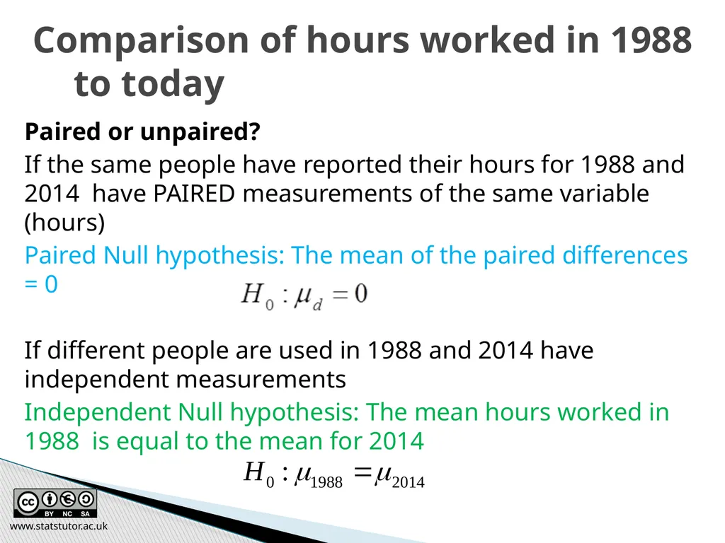
Paired or unpaired?
If the same people have reported their hours for 1988 and 2014 have PAIRED measurements of the same variable (hours)
Paired Null hypothesis: The mean of the paired differences = 0

If different people are used in 1988 and 2014 have independent measurements
Independent Null hypothesis: The mean hours worked in 1988 is equal to the mean for 2014 www.statstutor.ac.uk Comparison of hours worked in 1988 to today

60

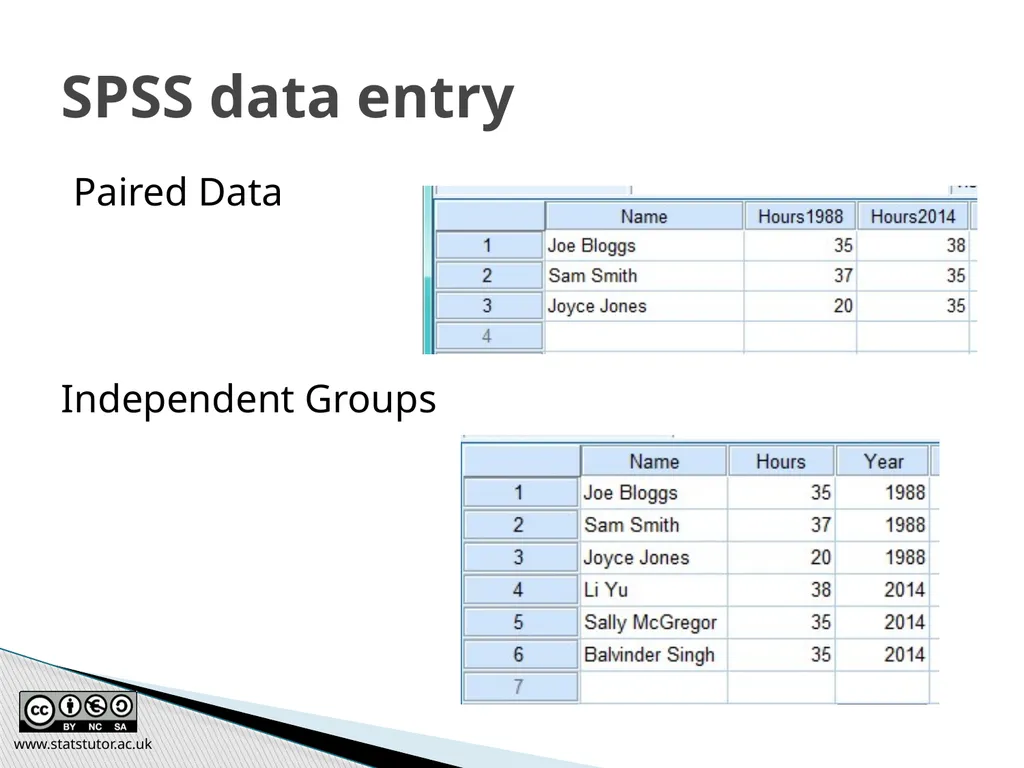
Paired Data

Independent Groups www.statstutor.ac.uk SPSS data entry

61

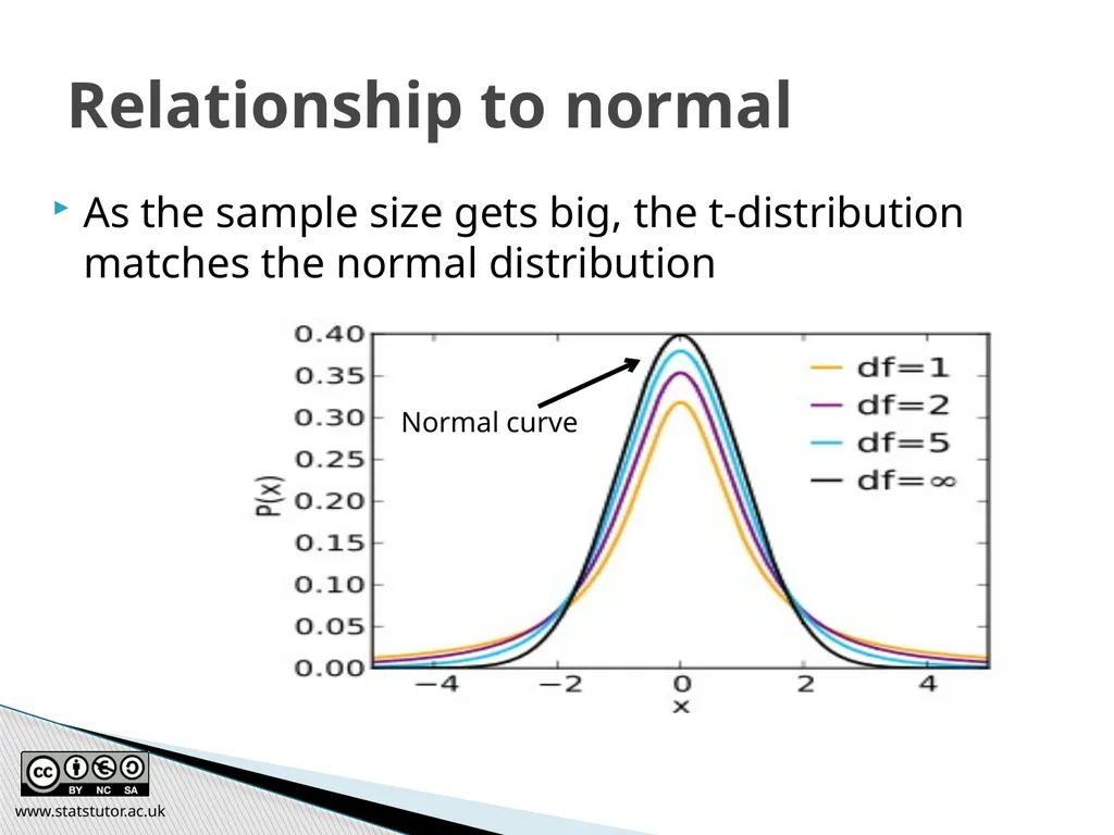
The t-distribution is similar to the standard normal distribution but has an additional parameter called degrees of freedom (df or v)

For a paired t-test, v = number of pairs – 1

For an independent t-test,

Used for small samples and when the population standard deviation is not known
Small sample sizes have heavier tails What is the t-distribution? www.statstutor.ac.uk

62

As the sample size gets big, the t-distribution matches the normal distribution Relationship to normal Normal curve www.statstutor.ac.uk

63

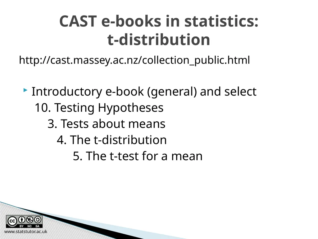
http://cast.massey.ac.nz/collection_public.html

Introductory e-book (general) and select
10. Testing Hypotheses
3. Tests about means
4. The t-distribution
5. The t-test for a mean www.statstutor.ac.uk CAST e-books in statistics:t-distribution

64

For Examples 1 and 2 (on the following four slides) discuss the answers to the following:

State a suitable null hypothesis
State whether it’s a Paired or Independent Samples t-test
Decide whether to reject the null hypothesis
State a conclusion in words www.statstutor.ac.uk Exercise

65

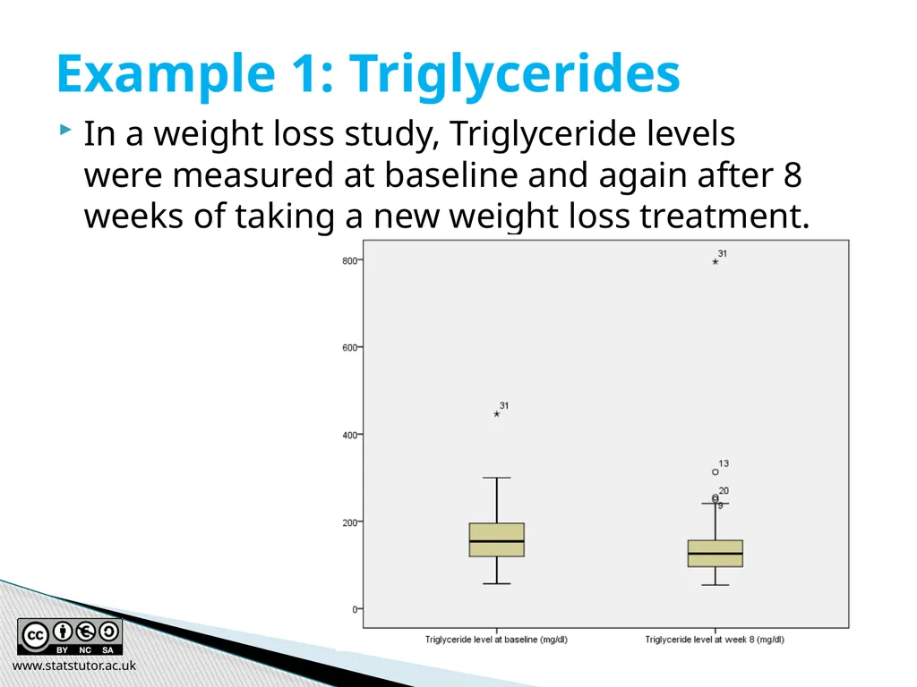
In a weight loss study, Triglyceride levels were measured at baseline and again after 8 weeks of taking a new weight loss treatment. www.statstutor.ac.uk Example 1: Triglycerides

66

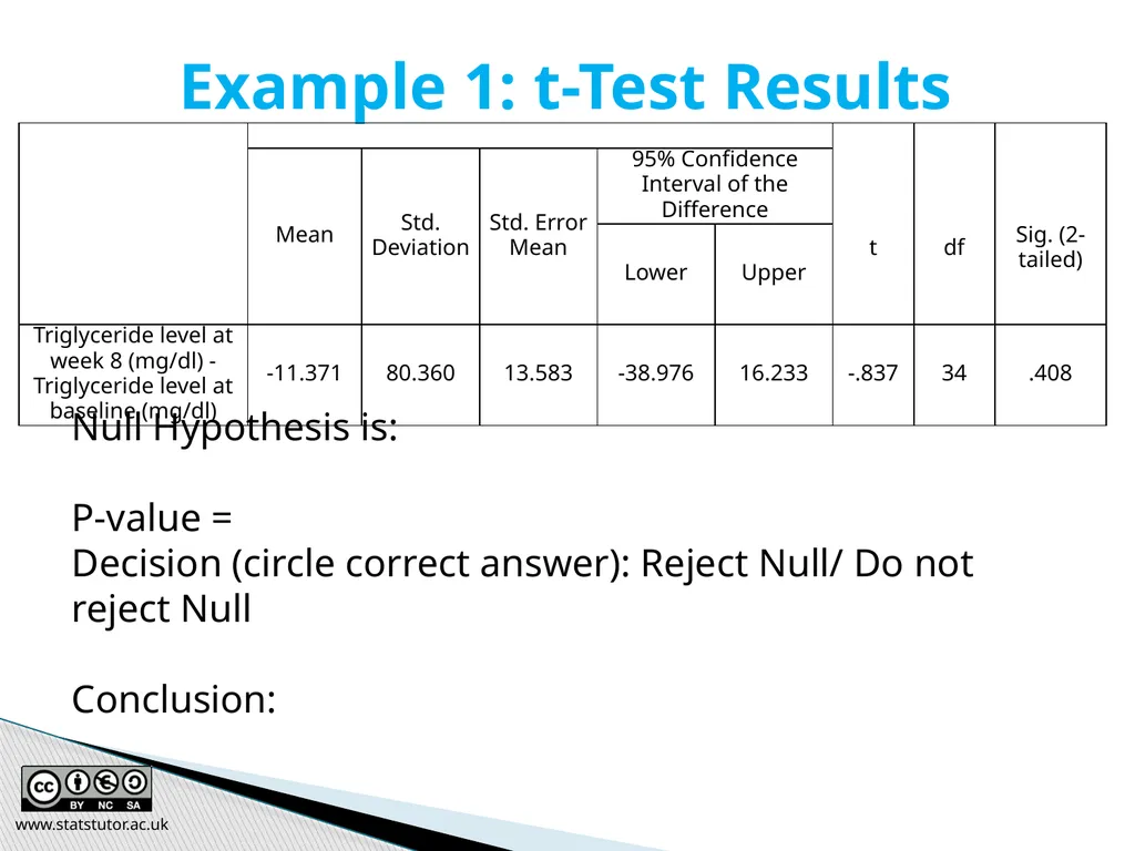
www.statstutor.ac.uk Example 1: t-Test Results Null Hypothesis is:

P-value =
Decision (circle correct answer): Reject Null/ Do not reject Null

Conclusion:

67

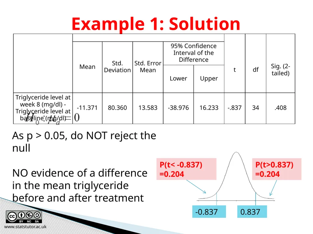
www.statstutor.ac.uk Example 1: Solution As p > 0.05, do NOT reject the null

NO evidence of a difference in the mean triglyceride before and after treatment

68

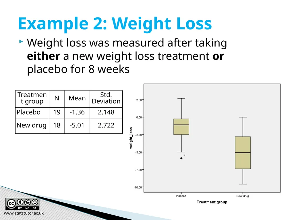
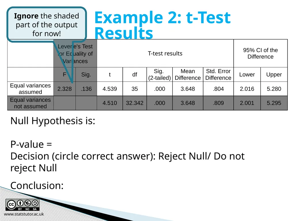
Weight loss was measured after taking either a new weight loss treatment or placebo for 8 weeks www.statstutor.ac.uk Example 2: Weight Loss

69

www.statstutor.ac.uk Example 2: t-Test Results Ignore the shaded part of the output for now! Null Hypothesis is:

P-value =
Decision (circle correct answer): Reject Null/ Do not reject Null

Conclusion:

70

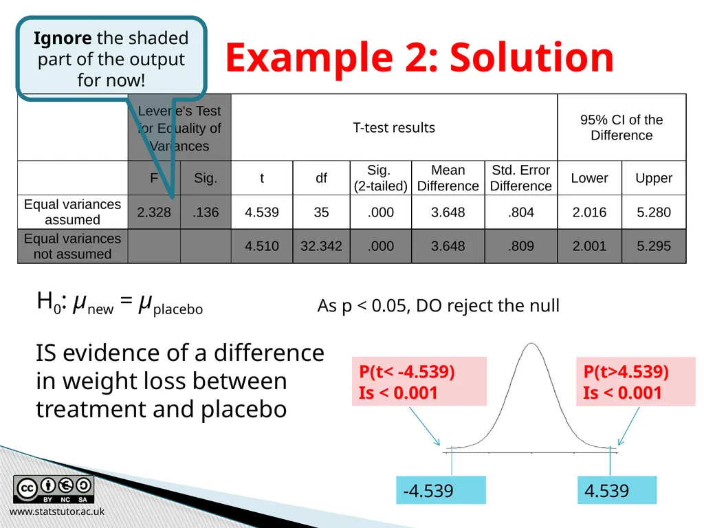
www.statstutor.ac.uk Example 2: Solution H0: μnew = μplacebo IS evidence of a difference in weight loss between treatment and placebo As p < 0.05, DO reject the null Ignore the shaded part of the output for now!

71

Every test has assumptions
Tutors quick guide shows assumptions for each test and what to do if those assumptions are not met www.statstutor.ac.uk Assumptions

72

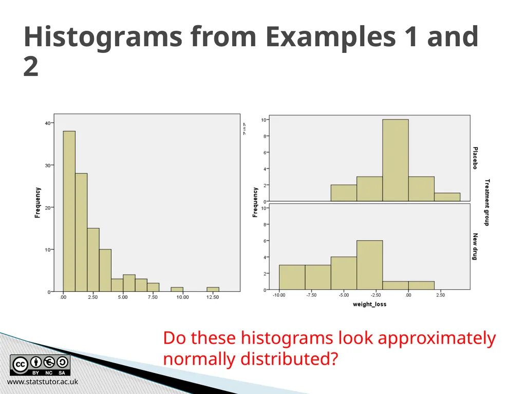
Normality: Plot histograms
One plot of the paired differences for any paired data
Two (One for each group) for independent samples
Don’t have to be perfect, just roughly symmetric

Equal Population variances: Compare sample standard deviations
As a rough estimate, one should be no more than twice the other
Do an F-test (Levene’s in SPSS) to formally test for differences

However the t-test is very robust to violations of the assumptions of Normality and equal variances, particularly for moderate (i.e. >30) and larger sample sizes www.statstutor.ac.uk Assumptions in t-Tests

73

www.statstutor.ac.uk Histograms from Examples 1 and 2 Do these histograms look approximately normally distributed?

74

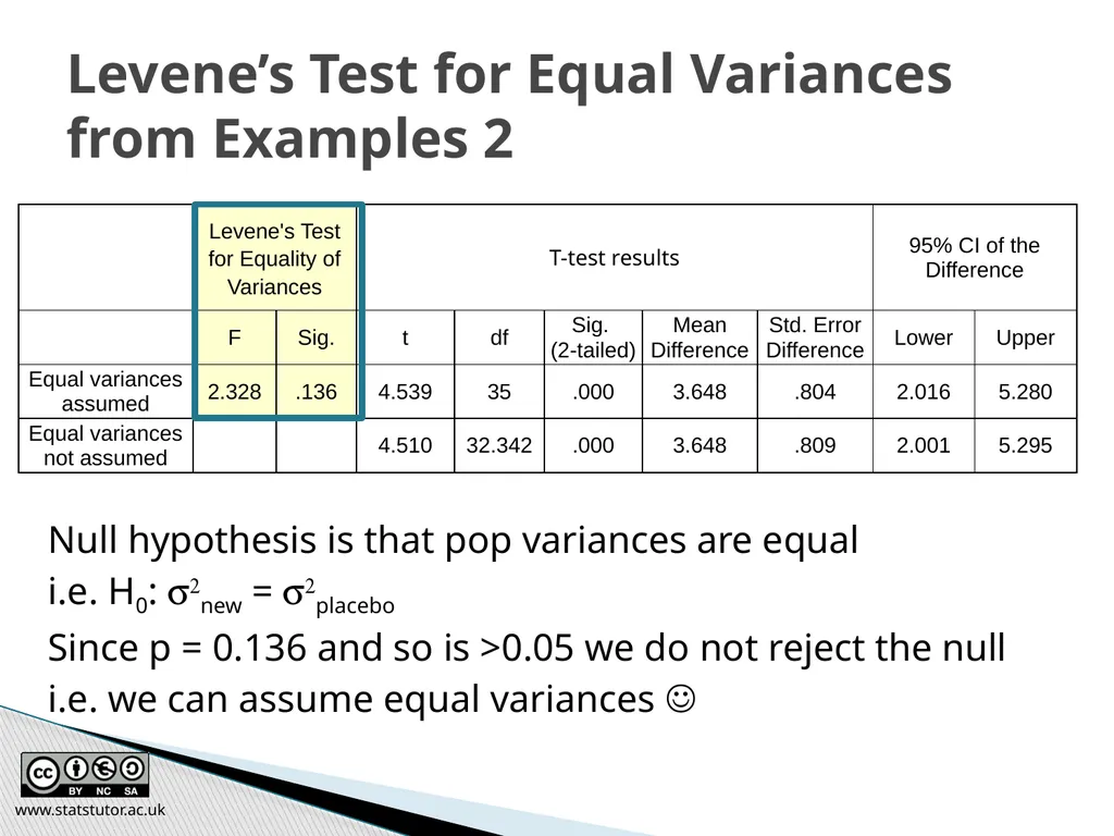
Null hypothesis is that pop variances are equal
i.e. H0: s2new = s2placebo
Since p = 0.136 and so is >0.05 we do not reject the null
i.e. we can assume equal variances  www.statstutor.ac.uk Levene’s Test for Equal Variances from Examples 2

75

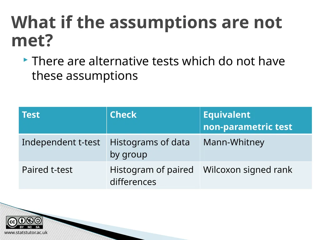
There are alternative tests which do not have these assumptions www.statstutor.ac.uk What if the assumptions are not met?

76

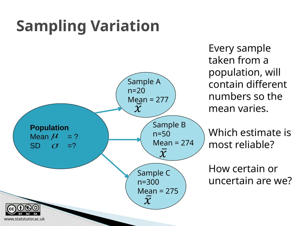
www.statstutor.ac.uk Sampling Variation Population
Mean = ?
SD =? Sample A
n=20
Mean = 277 Sample B
n=50
Mean = 274 Sample C
n=300
Mean = 275 Every sample taken from a population, will contain different numbers so the mean varies.

Which estimate is most reliable?

How certain or uncertain are we?

77

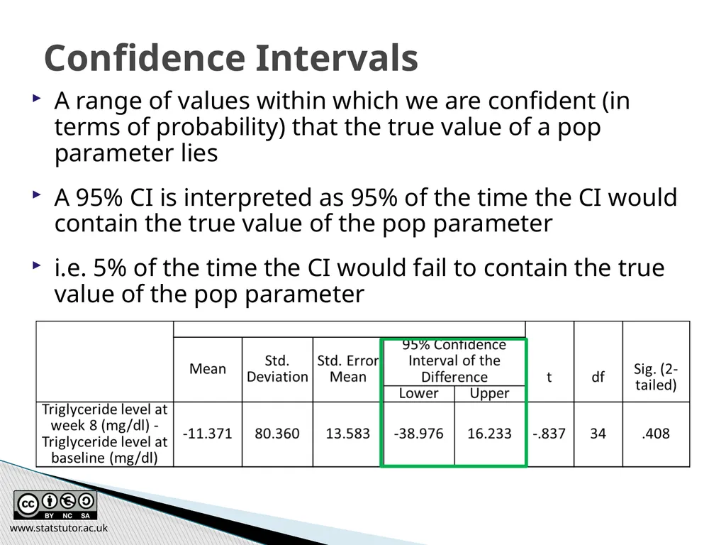
A range of values within which we are confident (in terms of probability) that the true value of a pop parameter lies
A 95% CI is interpreted as 95% of the time the CI would contain the true value of the pop parameter
i.e. 5% of the time the CI would fail to contain the true value of the pop parameter www.statstutor.ac.uk Confidence Intervals

78

http://cast.massey.ac.nz/collection_public.html

Choose introductory e-book (general) and select
9. Estimating Parameters
3. Conf. Interval for mean
6. Properties of 95% C.I. www.statstutor.ac.uk CAST e-books in statistics:Confidence Intervals

79

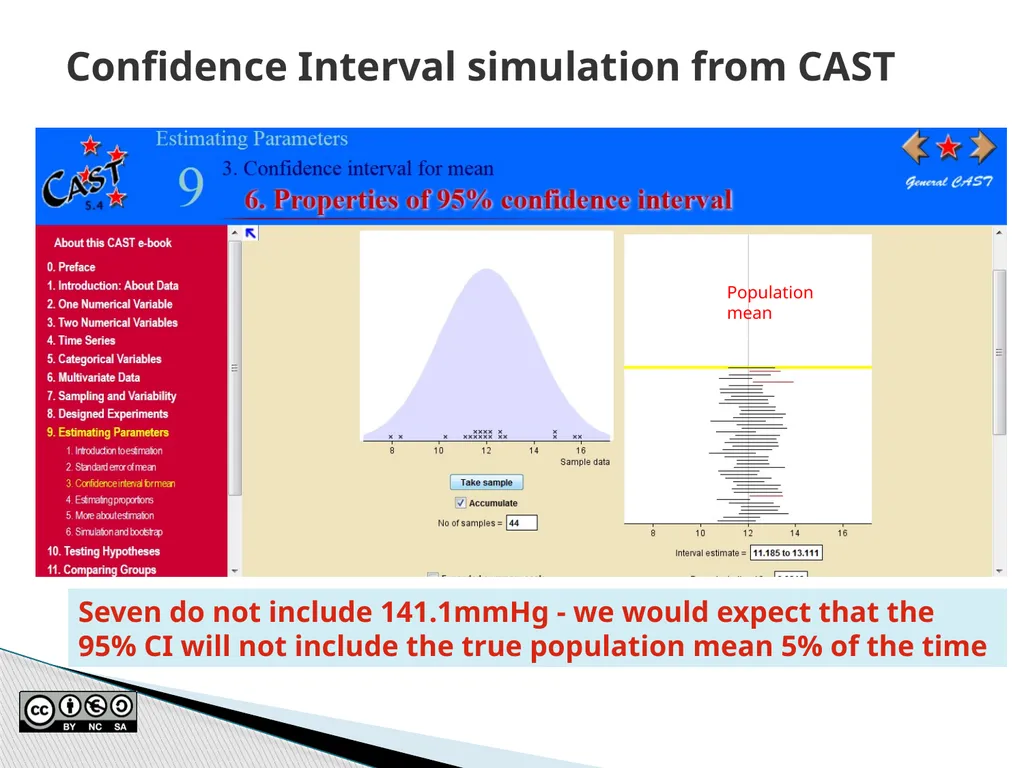
Confidence Interval simulation from CAST Seven do not include 141.1mmHg - we would expect that the 95% CI will not include the true population mean 5% of the time Population mean

80

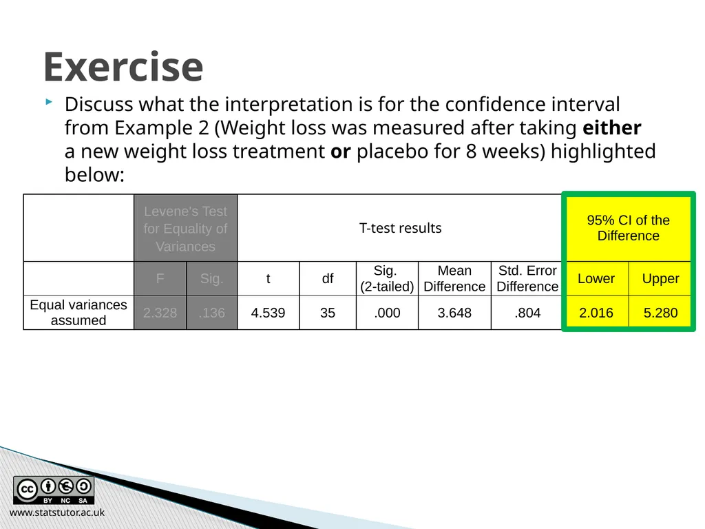
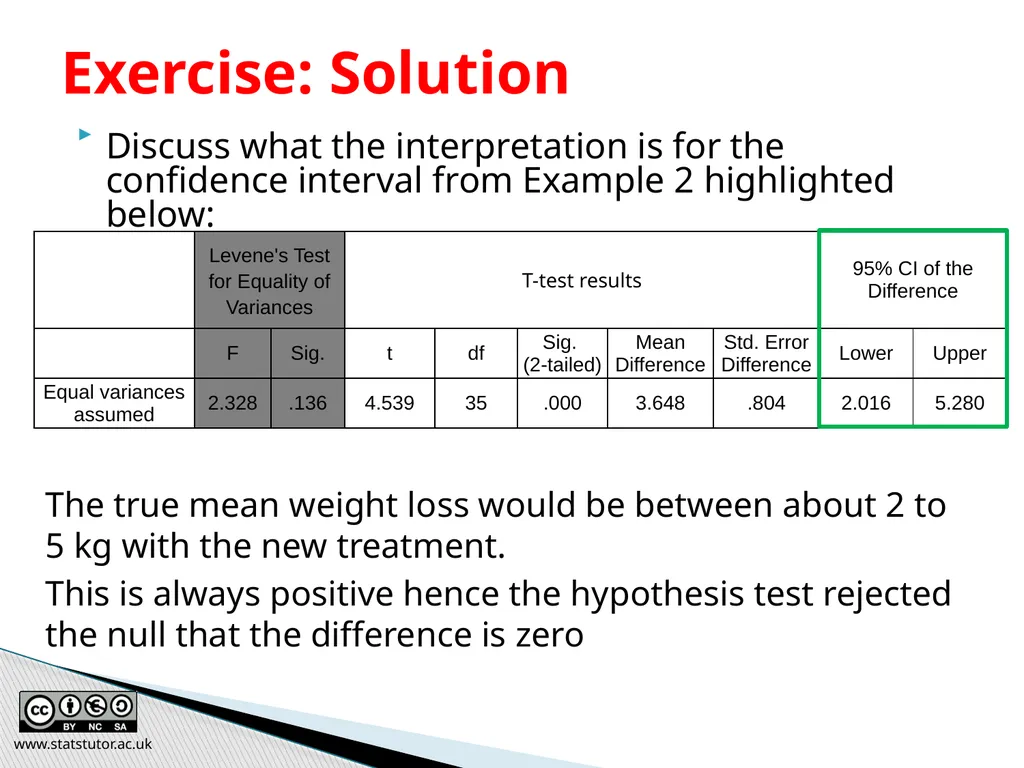
Discuss what the interpretation is for the confidence interval from Example 2 (Weight loss was measured after taking either a new weight loss treatment or placebo for 8 weeks) highlighted below: www.statstutor.ac.uk Exercise

81

Discuss what the interpretation is for the confidence interval from Example 2 highlighted below: www.statstutor.ac.uk Exercise: Solution The true mean weight loss would be between about 2 to 5 kg with the new treatment.
This is always positive hence the hypothesis test rejected the null that the difference is zero

82

Investigating relationships www.statstutor.ac.uk Ellen Marshall / Alun Owen
University of Sheffield / University of Worcester Reviewer: Ruth Fairclough
University of Wolverhampton community project
encouraging academics to share statistics support resources
All stcp resources are released under a Creative Commons licence

83

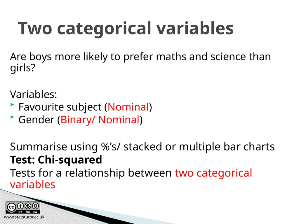
Are boys more likely to prefer maths and science than girls?

Variables:
Favourite subject (Nominal)
Gender (Binary/ Nominal)

Summarise using %’s/ stacked or multiple bar charts
Test: Chi-squared
Tests for a relationship between two categorical variables www.statstutor.ac.uk Two categorical variables

84

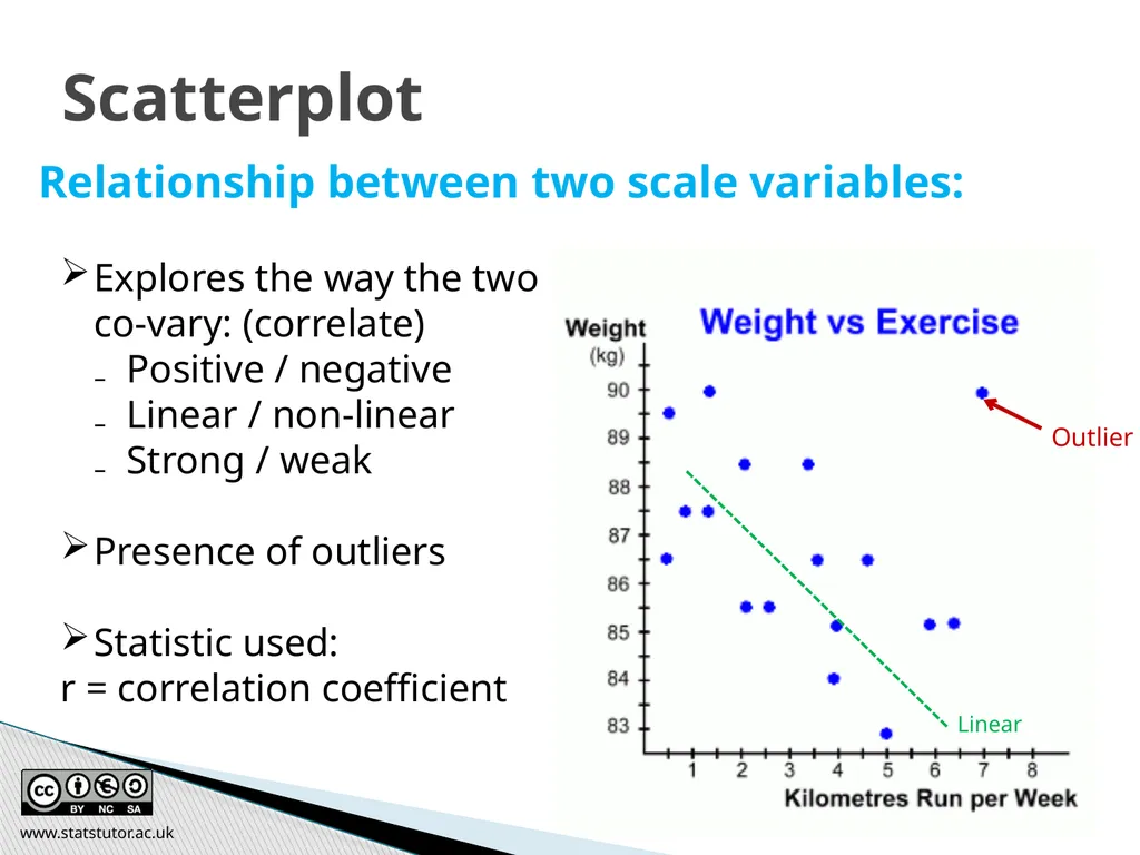
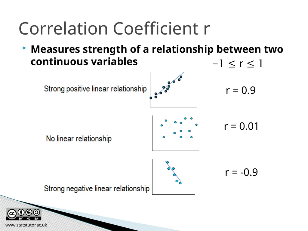
Relationship between two scale variables: Scatterplot Outlier Linear Explores the way the two co-vary: (correlate)
Positive / negative
Linear / non-linear
Strong / weak

Presence of outliers

Statistic used:
r = correlation coefficient www.statstutor.ac.uk

85

Correlation Coefficient r Measures strength of a relationship between two continuous variables r = 0.9 r = 0.01 r = -0.9 www.statstutor.ac.uk

86

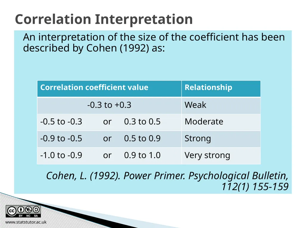
An interpretation of the size of the coefficient has been described by Cohen (1992) as:

Cohen, L. (1992). Power Primer. Psychological Bulletin, 112(1) 155-159 Correlation Interpretation www.statstutor.ac.uk

87

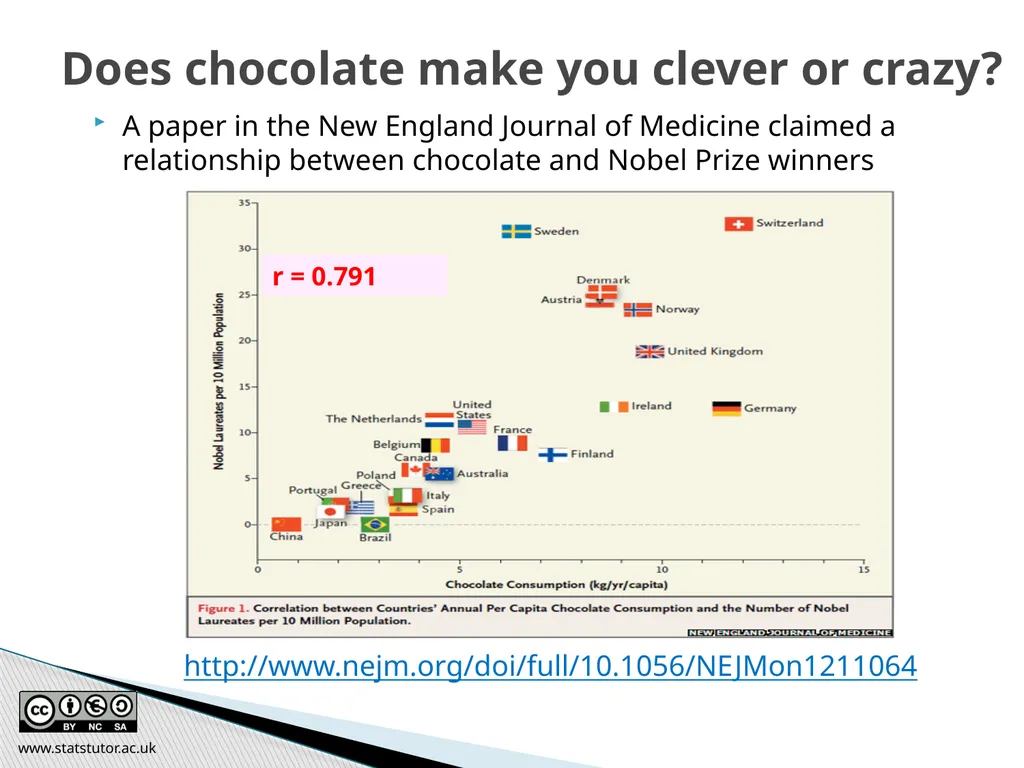
Does chocolate make you clever or crazy? A paper in the New England Journal of Medicine claimed a relationship between chocolate and Nobel Prize winners

http://www.nejm.org/doi/full/10.1056/NEJMon1211064 r = 0.791 www.statstutor.ac.uk

88

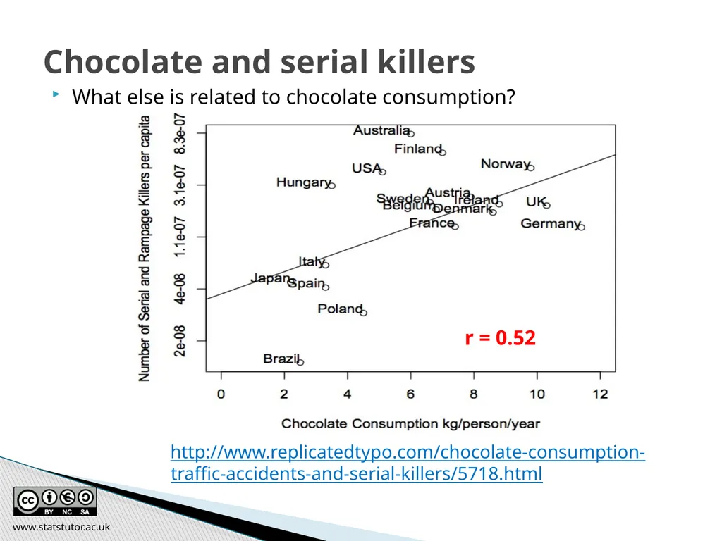
Chocolate and serial killers What else is related to chocolate consumption?

http://www.replicatedtypo.com/chocolate-consumption-traffic-accidents-and-serial-killers/5718.html r = 0.52 www.statstutor.ac.uk

89

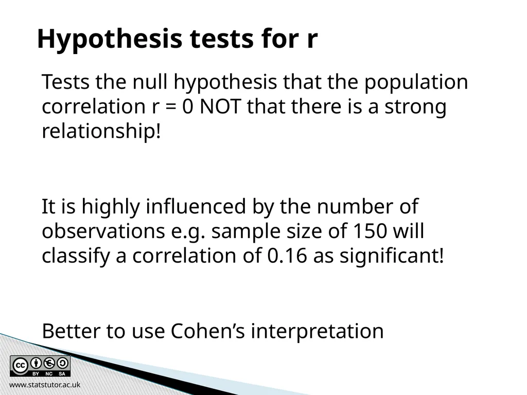
Tests the null hypothesis that the population correlation r = 0 NOT that there is a strong relationship!

It is highly influenced by the number of observations e.g. sample size of 150 will classify a correlation of 0.16 as significant!

Better to use Cohen’s interpretation Hypothesis tests for r www.statstutor.ac.uk

90

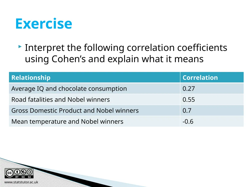
Interpret the following correlation coefficients using Cohen’s and explain what it means Exercise www.statstutor.ac.uk

91

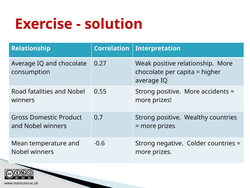
Exercise - solution www.statstutor.ac.uk

92

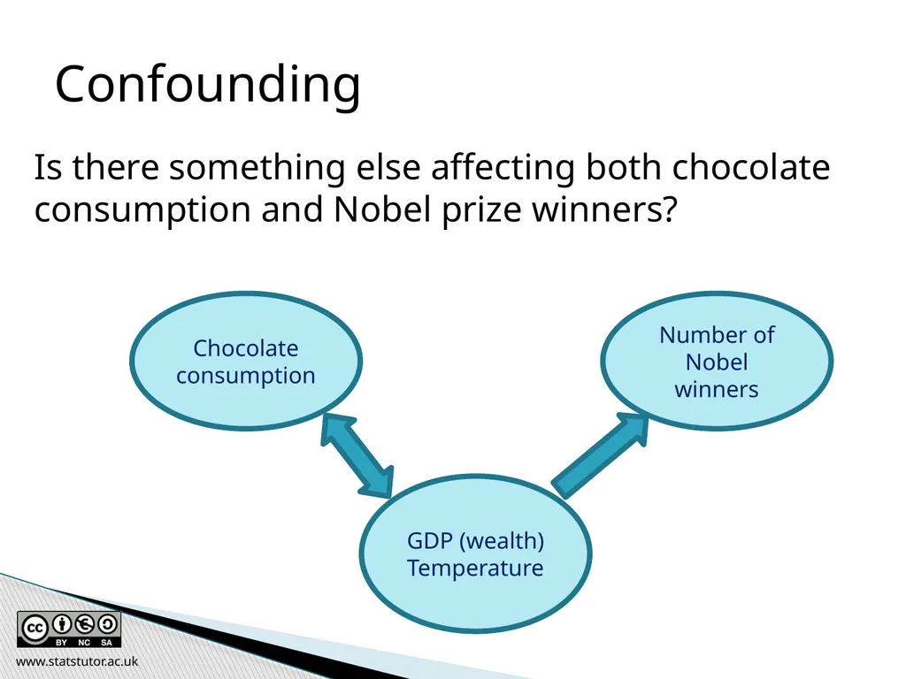
Confounding Is there something else affecting both chocolate consumption and Nobel prize winners? Chocolate consumption Number of Nobel winners GDP (wealth)
Temperature www.statstutor.ac.uk

93

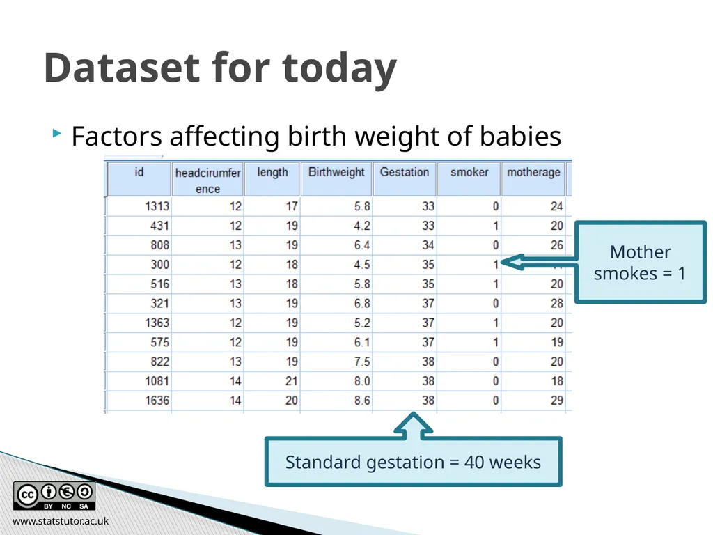
Factors affecting birth weight of babies Dataset for today Standard gestation = 40 weeks Mother smokes = 1 www.statstutor.ac.uk

94

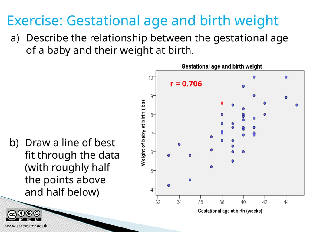
Exercise: Gestational age and birth weight Describe the relationship between the gestational age of a baby and their weight at birth. Draw a line of best fit through the data (with roughly half the points above and half below) r = 0.706 www.statstutor.ac.uk

95

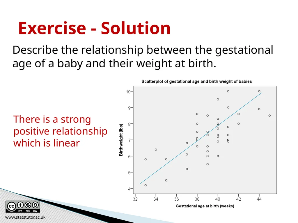
Describe the relationship between the gestational age of a baby and their weight at birth. Exercise - Solution There is a strong positive relationship which is linear www.statstutor.ac.uk

96

Regression is useful when we want to
look for significant relationships between two variables
predict a value of one variable for a given value of the other

It involves estimating the line of best fit through the data which minimises the sum of the squared residuals

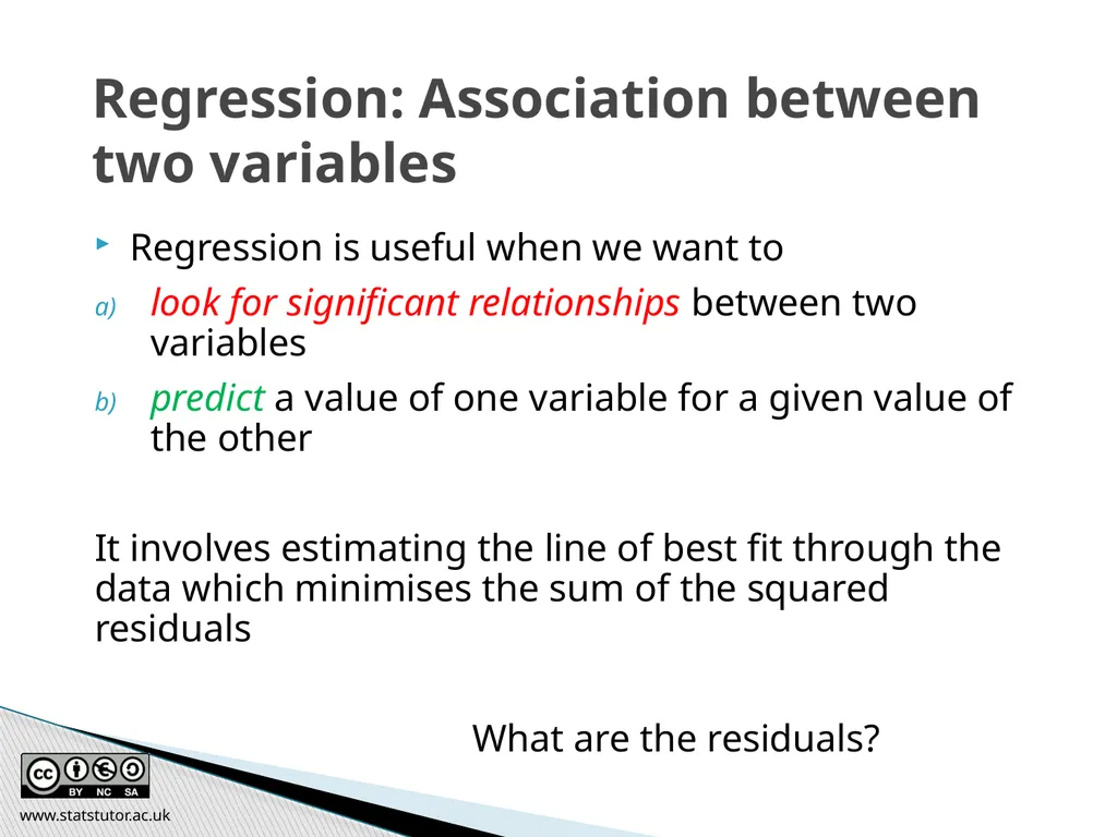
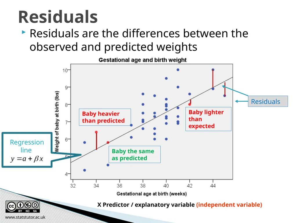
What are the residuals? Regression: Association between two variables www.statstutor.ac.uk

97

Residuals are the differences between the observed and predicted weights Residuals Baby heavier than predicted Baby lighter than expected Residuals Baby the same as predicted X Predictor / explanatory variable (independent variable) Regression line www.statstutor.ac.uk

98

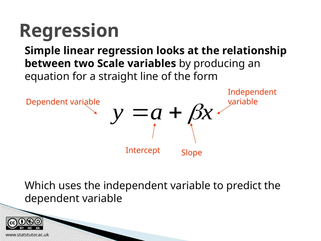
Simple linear regression looks at the relationship between two Scale variables by producing an equation for a straight line of the form

Which uses the independent variable to predict the dependent variable Regression Intercept Slope Dependent variable Independent variable www.statstutor.ac.uk

99

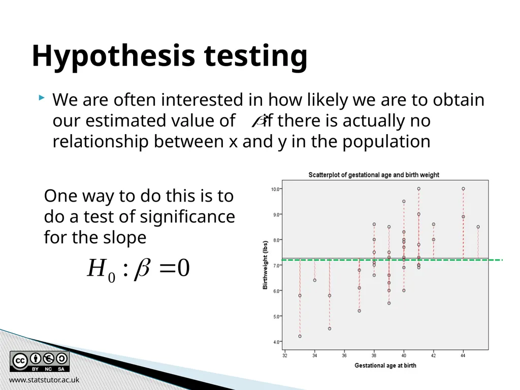
Hypothesis testing We are often interested in how likely we are to obtain our estimated value of if there is actually no relationship between x and y in the population One way to do this is to do a test of significance for the slope www.statstutor.ac.uk

100

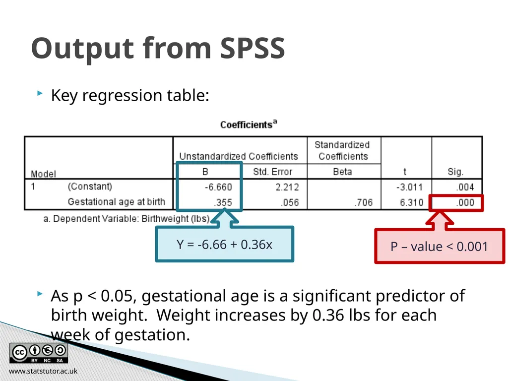
Output from SPSS Key regression table:

As p < 0.05, gestational age is a significant predictor of birth weight. Weight increases by 0.36 lbs for each week of gestation. Y = -6.66 + 0.36x P – value < 0.001 www.statstutor.ac.uk

101

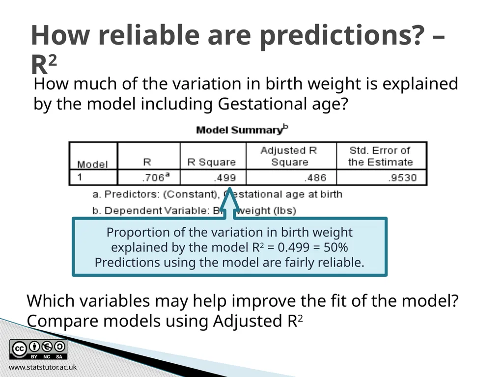
How much of the variation in birth weight is explained by the model including Gestational age? How reliable are predictions? – R2 Proportion of the variation in birth weight explained by the model R2 = 0.499 = 50%
Predictions using the model are fairly reliable. Which variables may help improve the fit of the model?
Compare models using Adjusted R2 www.statstutor.ac.uk

102

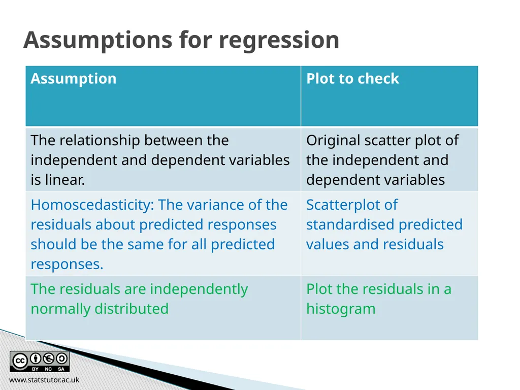
Assumptions for regression Look for patterns. www.statstutor.ac.uk

103

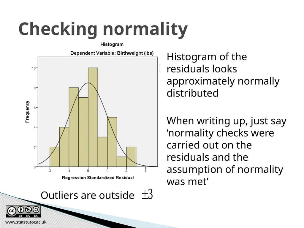
Histogram of the residuals looks approximately normally distributed

When writing up, just say ‘normality checks were carried out on the residuals and the assumption of normality was met’ Checking normality Outliers are outside www.statstutor.ac.uk

104

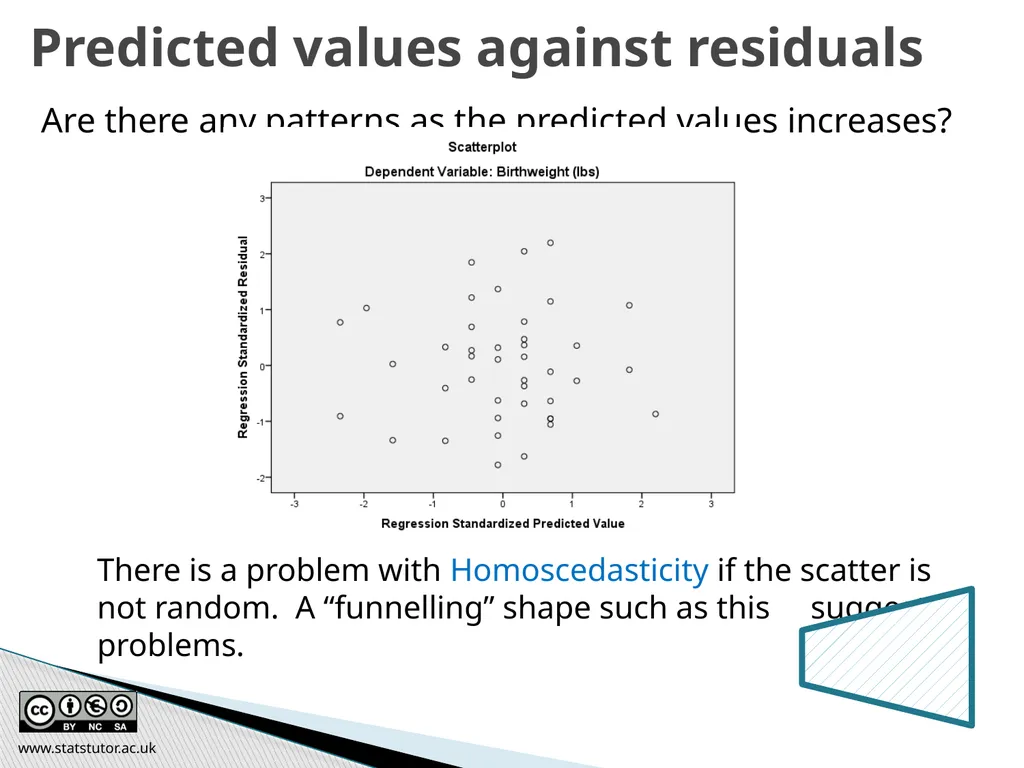
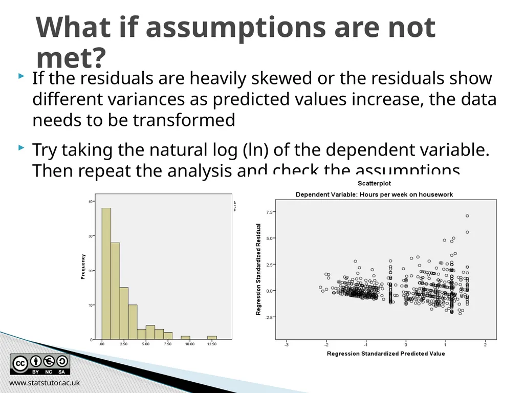
Predicted values against residuals There is a problem with Homoscedasticity if the scatter is not random. A “funnelling” shape such as this suggests problems. Are there any patterns as the predicted values increases? www.statstutor.ac.uk

105

What if assumptions are not met? If the residuals are heavily skewed or the residuals show different variances as predicted values increase, the data needs to be transformed
Try taking the natural log (ln) of the dependent variable. Then repeat the analysis and check the assumptions www.statstutor.ac.uk

106

Investigate whether mothers pre-pregnancy weight and birth weight are associated using a scatterplot, correlation and simple regression. Exercise www.statstutor.ac.uk

107

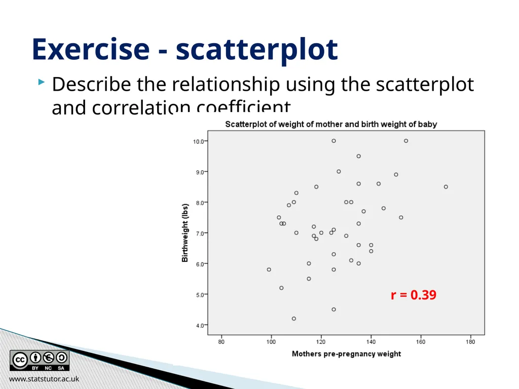
Describe the relationship using the scatterplot and correlation coefficient Exercise - scatterplot r = 0.39 www.statstutor.ac.uk

108

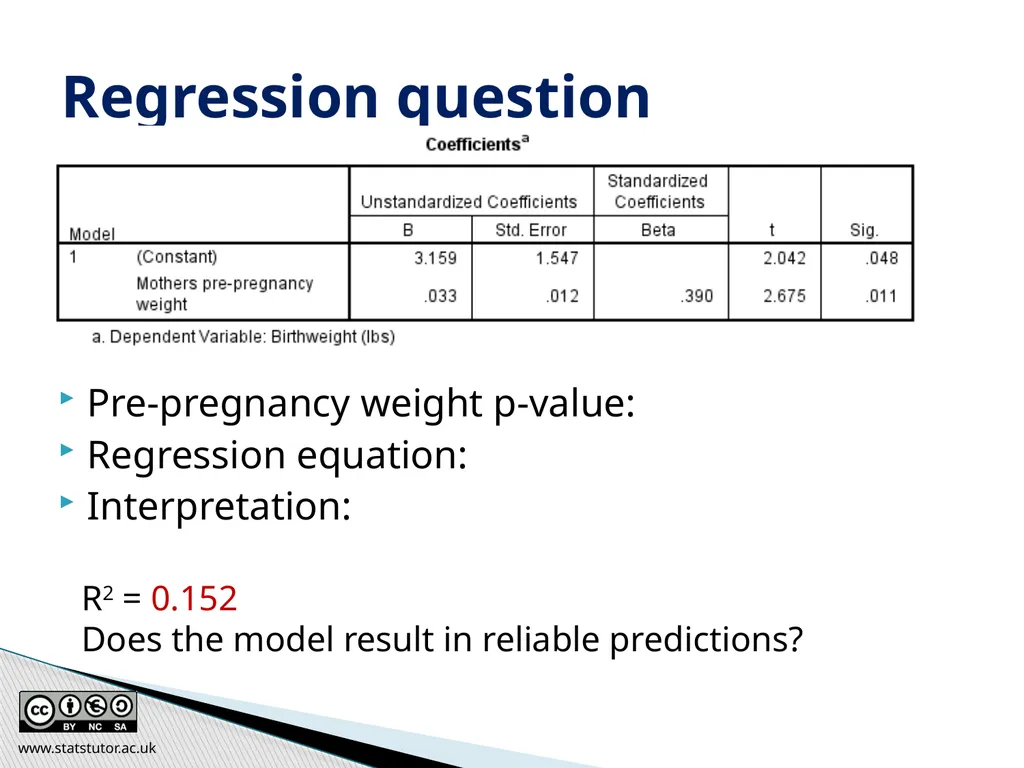
Pre-pregnancy weight p-value:
Regression equation:
Interpretation: Regression question R2 = 0.152
Does the model result in reliable predictions? www.statstutor.ac.uk

109

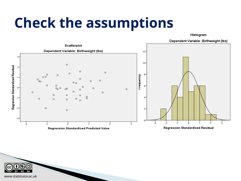
Check the assumptions www.statstutor.ac.uk

110

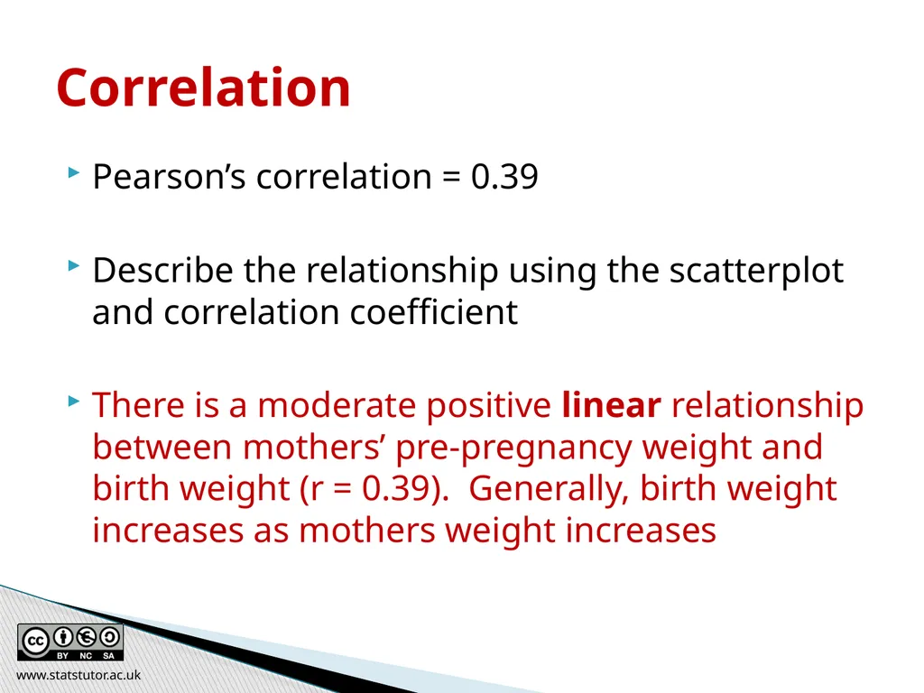
Pearson’s correlation = 0.39

Describe the relationship using the scatterplot and correlation coefficient

There is a moderate positive linear relationship between mothers’ pre-pregnancy weight and birth weight (r = 0.39). Generally, birth weight increases as mothers weight increases Correlation www.statstutor.ac.uk

111

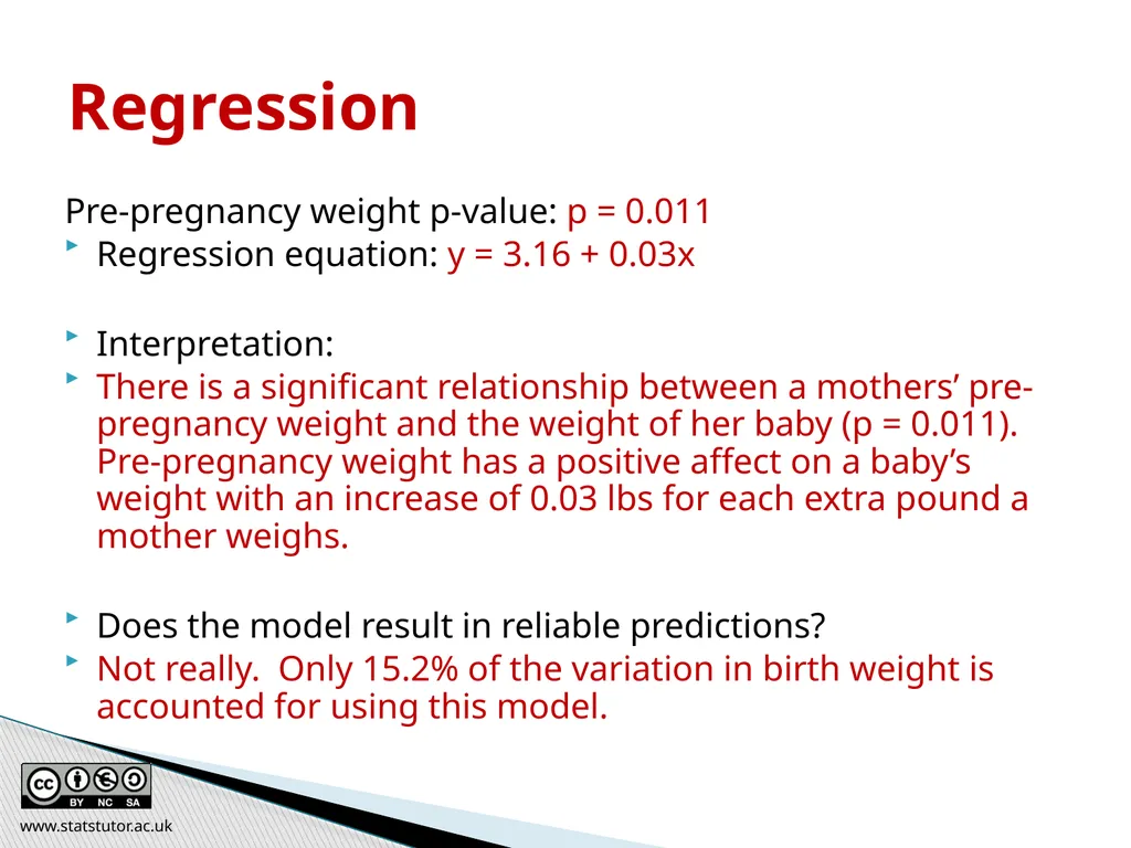
Pre-pregnancy weight p-value: p = 0.011
Regression equation: y = 3.16 + 0.03x

Interpretation:
There is a significant relationship between a mothers’ pre-pregnancy weight and the weight of her baby (p = 0.011). Pre-pregnancy weight has a positive affect on a baby’s weight with an increase of 0.03 lbs for each extra pound a mother weighs.

Does the model result in reliable predictions?
Not really. Only 15.2% of the variation in birth weight is accounted for using this model. Regression www.statstutor.ac.uk

112

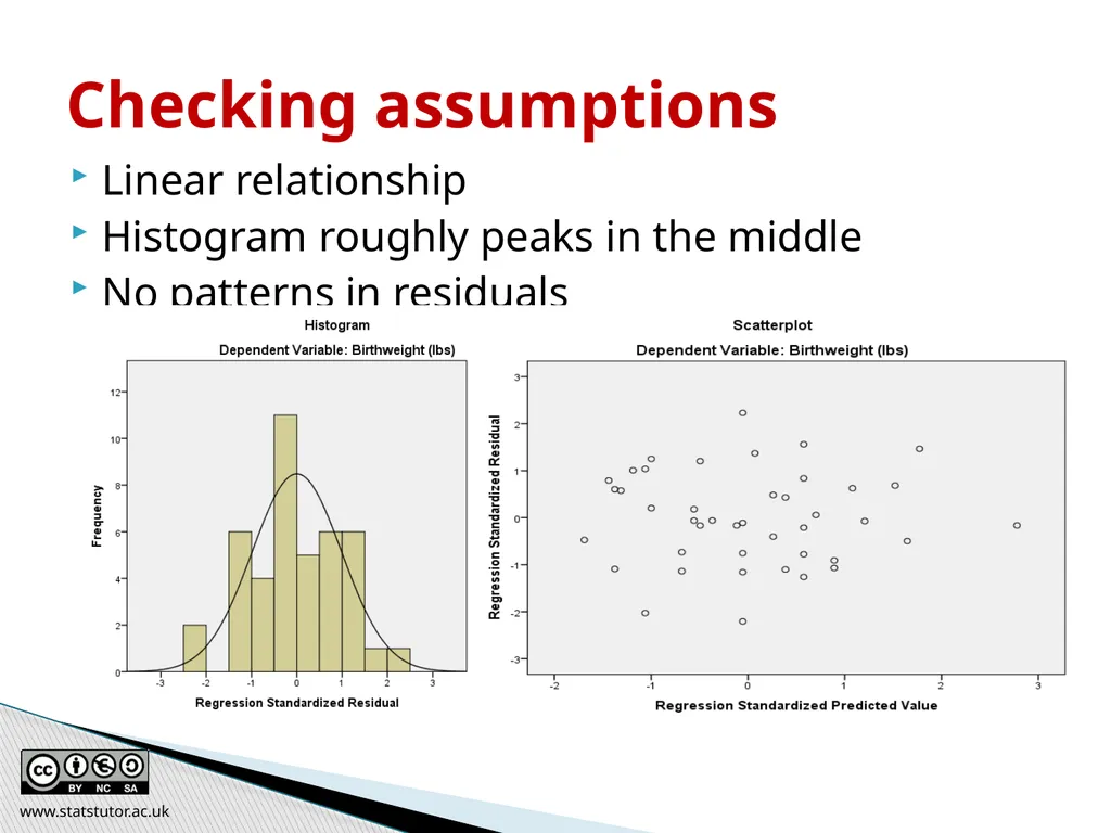
Linear relationship
Histogram roughly peaks in the middle
No patterns in residuals Checking assumptions www.statstutor.ac.uk

113

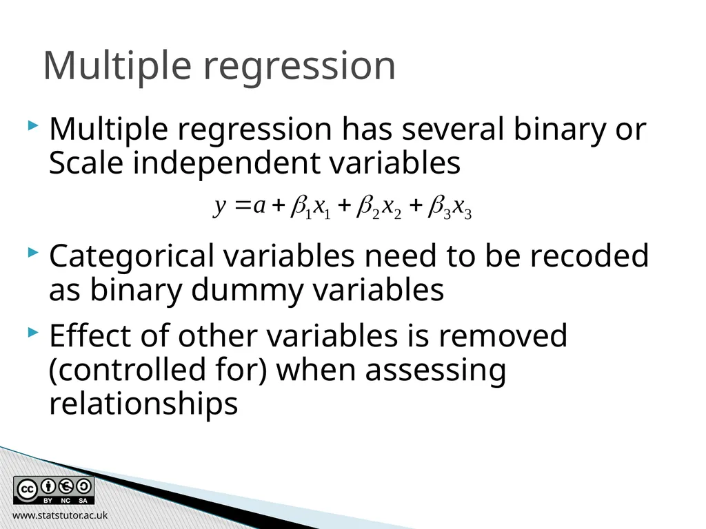
Multiple regression Multiple regression has several binary or Scale independent variables

Categorical variables need to be recoded as binary dummy variables
Effect of other variables is removed (controlled for) when assessing relationships www.statstutor.ac.uk

114

Multiple regression What affects the number of Nobel prize winners?

Dependent: Number of Nobel prize winners

Possible independents: Chocolate consumption, GDP and mean temperature

Chocolate consumption is significantly related to Nobel prize winners in simple linear regression
Once the effect of a country’s GDP and temperature were taken into account, there was no relationship www.statstutor.ac.uk

115

In addition to the standard linear regression checks, relationships BETWEEN independent variables should be assessed
Multicollinearity is a problem where continuous independent variables are too correlated (r > 0.8)
Relationships can be assessed using scatterplots and correlation for scale variables
SPSS can also report collinearity statistics on request. The VIF should be close to 1 but under 5 is fine whereas 10 + needs checking Multiple regression www.statstutor.ac.uk

116

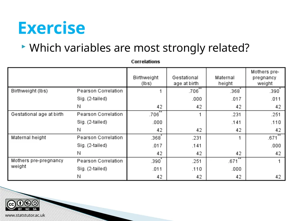
Which variables are most strongly related? Exercise www.statstutor.ac.uk

117

Which variables are most strongly related?
Gestation and birth weight (0.709)

Mothers height and weight (0.671)
Mothers height and weight are strongly related. They don’t exceed the problem correlation of 0.8 but try the model with and without height in case it’s a problem.
When both were included in regression, neither were significant but alone they were Exercise - Solution www.statstutor.ac.uk

118

Logistic regression Logistic regression has a binary dependent variable
The model can be used to estimate probabilities

Example: insurance quotes are based on the likelihood of you having an accident
Dependent = Have an accident/ do not have accident
Independents: Age (preferably Scale), gender, occupation, marital status, annual mileage

Ordinal regression is for ordinal dependent variables www.statstutor.ac.uk

119

Choosing the right test www.statstutor.ac.uk Ellen Marshall / Alun Owen
University of Sheffield / University of Worcester Reviewer: Ruth Fairclough
University of Wolverhampton community project
encouraging academics to share statistics support resources
All stcp resources are released under a Creative Commons licence

120

Choosing the right test One of the most common queries in stats support is ‘Which analysis should I use’

There are several steps to help the student decide

When a student is explaining their project, these are the questions you need answers for www.statstutor.ac.uk

121

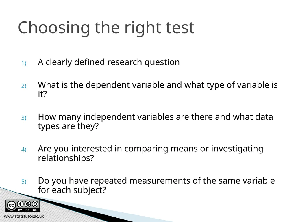
Choosing the right test A clearly defined research question

What is the dependent variable and what type of variable is it?

How many independent variables are there and what data types are they?

Are you interested in comparing means or investigating relationships?

Do you have repeated measurements of the same variable for each subject? www.statstutor.ac.uk

122

Clear questions with measurable quantities

Which variables will help answer these questions

Think about what test is needed before carrying out a study so that the right type of variables are collected Research question www.statstutor.ac.uk

123

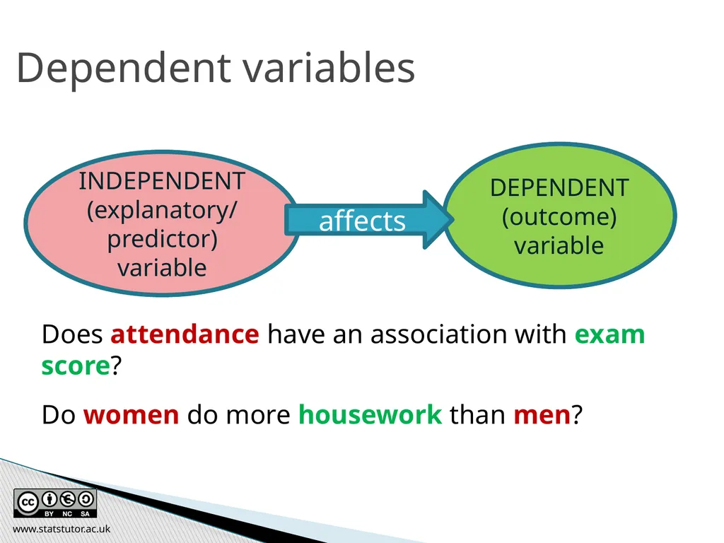
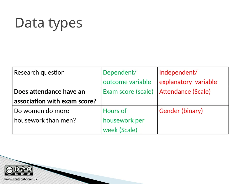
Dependent variables Does attendance have an association with exam score?
Do women do more housework than men? www.statstutor.ac.uk

124

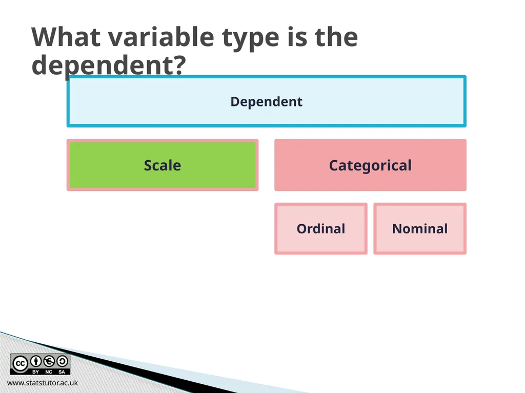
What variable type is the dependent? www.statstutor.ac.uk

125

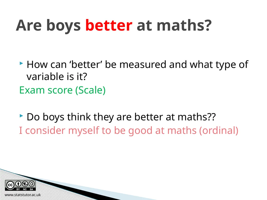
How can ‘better’ be measured and what type of variable is it?
Exam score (Scale)

Do boys think they are better at maths??
I consider myself to be good at maths (ordinal) Are boys better at maths? www.statstutor.ac.uk

126

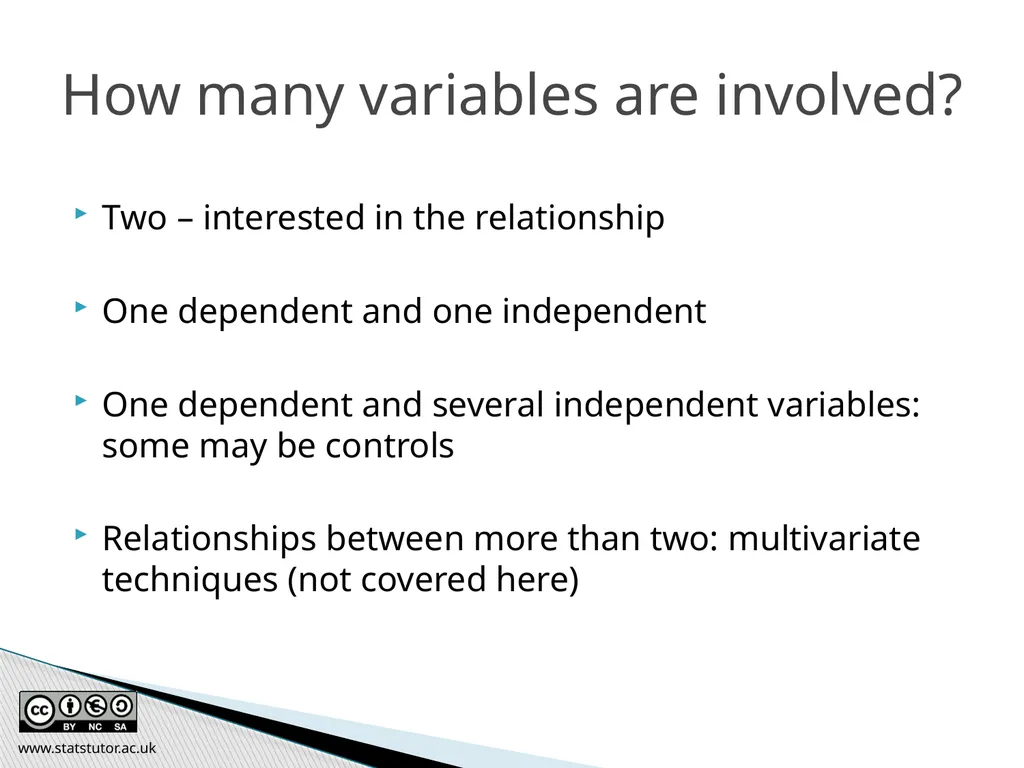
How many variables are involved? Two – interested in the relationship

One dependent and one independent

One dependent and several independent variables: some may be controls

Relationships between more than two: multivariate techniques (not covered here) www.statstutor.ac.uk

127

Data types www.statstutor.ac.uk

128

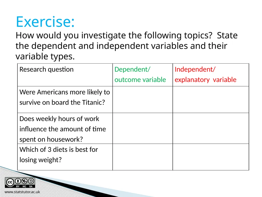
Exercise: How would you investigate the following topics? State the dependent and independent variables and their variable types. www.statstutor.ac.uk

129

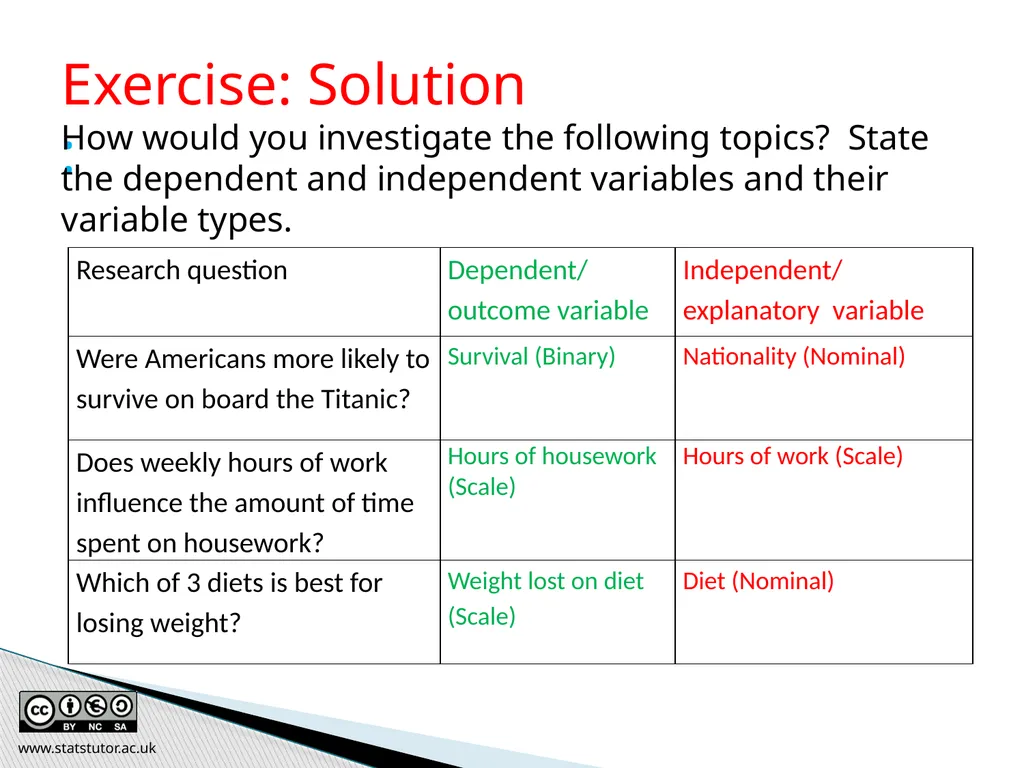
Exercise: Solution
: How would you investigate the following topics? State the dependent and independent variables and their variable types. www.statstutor.ac.uk

130

Dependent = Scale
Independent = Categorical

How many means are you comparing?

Do you have independent groups or repeated measurements on each person? Comparing means www.statstutor.ac.uk

131

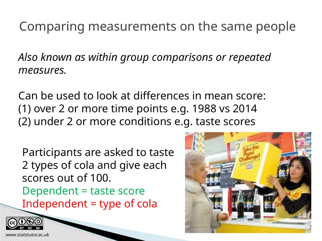
Comparing measurements on the same people Also known as within group comparisons or repeated measures.

Can be used to look at differences in mean score:
over 2 or more time points e.g. 1988 vs 2014
(2) under 2 or more conditions e.g. taste scores Participants are asked to taste 2 types of cola and give each scores out of 100.
Dependent = taste score
Independent = type of cola www.statstutor.ac.uk

132

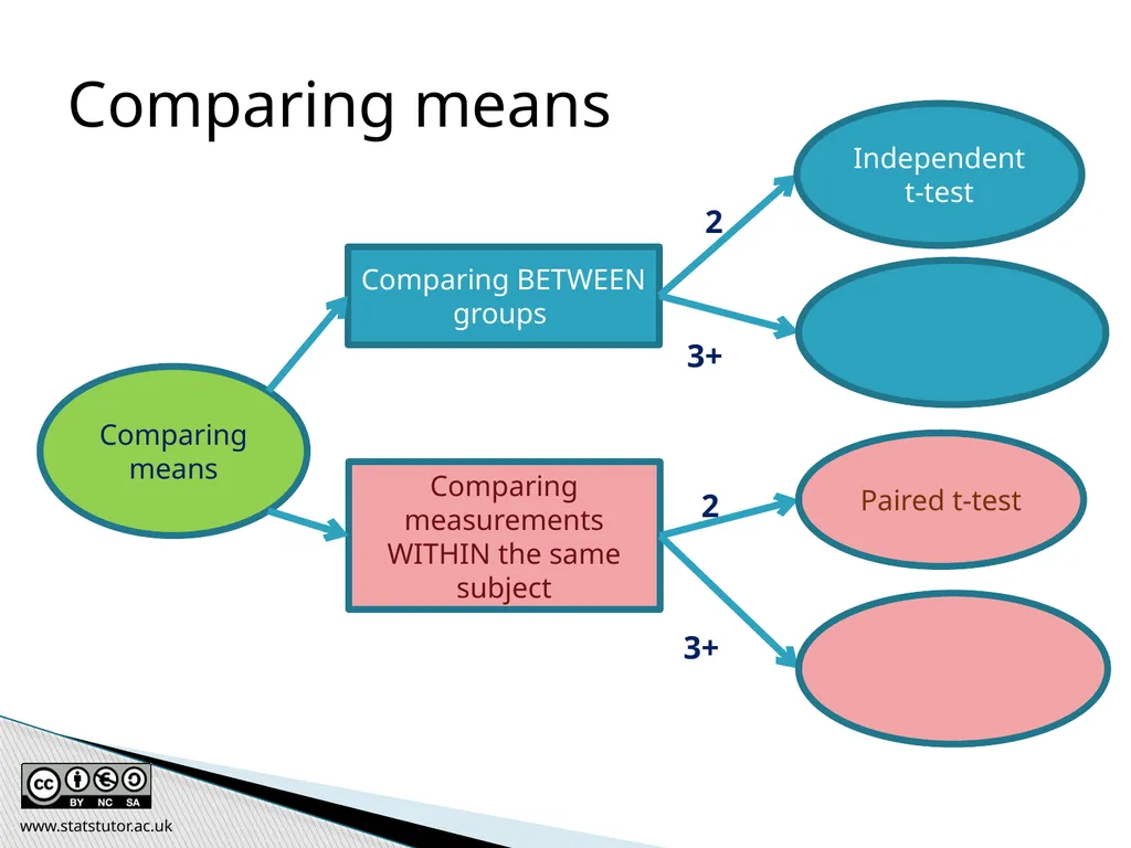
Comparing means Comparing means Comparing BETWEEN groups Comparing measurements WITHIN the same subject 3+ 2 Paired t-test 3+ www.statstutor.ac.uk

133

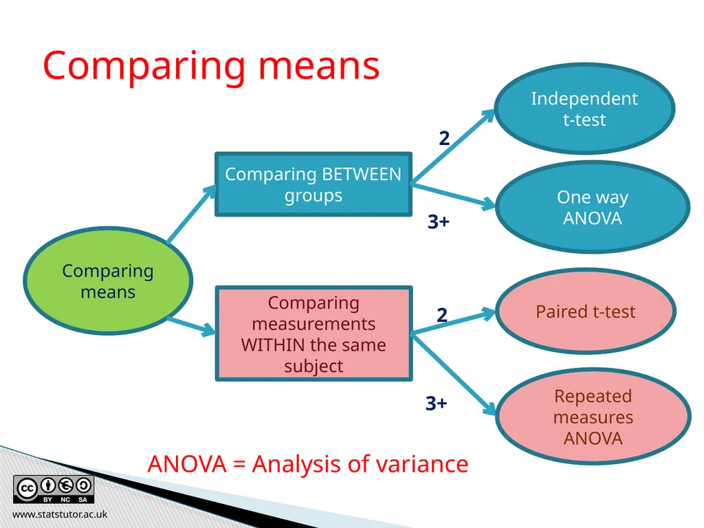
Comparing means Comparing means Comparing BETWEEN groups Comparing measurements WITHIN the same subject 3+ 2 Paired t-test Repeated measures ANOVA 3+ ANOVA = Analysis of variance www.statstutor.ac.uk

134

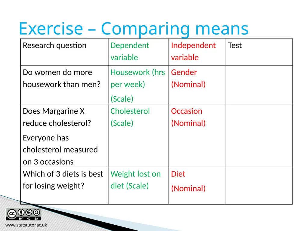
Exercise – Comparing means www.statstutor.ac.uk

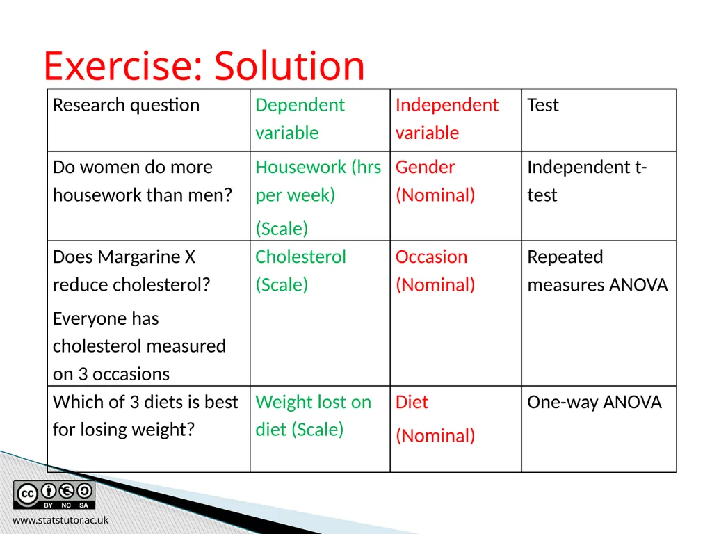
135

Exercise: Solution www.statstutor.ac.uk

136

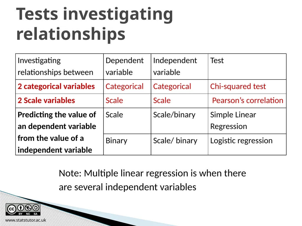
Tests investigating relationships Note: Multiple linear regression is when there are several independent variables www.statstutor.ac.uk

137

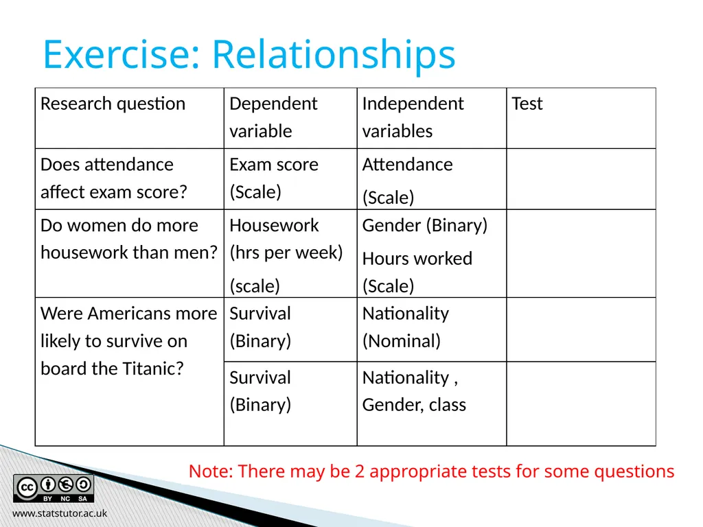
Exercise: Relationships Note: There may be 2 appropriate tests for some questions www.statstutor.ac.uk

138

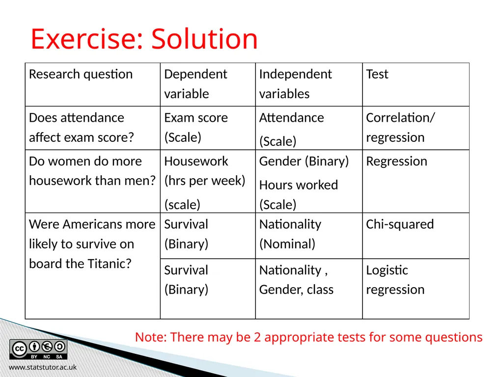
Exercise: Solution Note: There may be 2 appropriate tests for some questions www.statstutor.ac.uk

139

Non-parametric tests www.statstutor.ac.uk Ellen Marshall / Alun Owen
University of Sheffield / University of Worcester Reviewer: Ruth Fairclough
University of Wolverhampton community project
encouraging academics to share statistics support resources
All stcp resources are released under a Creative Commons licence

140

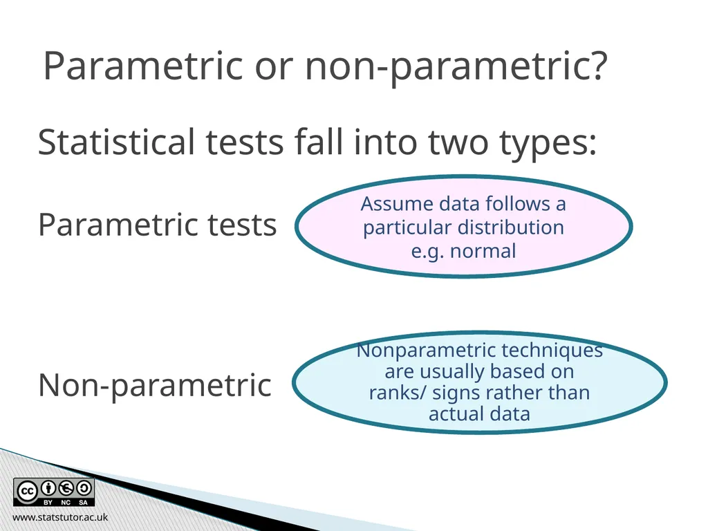
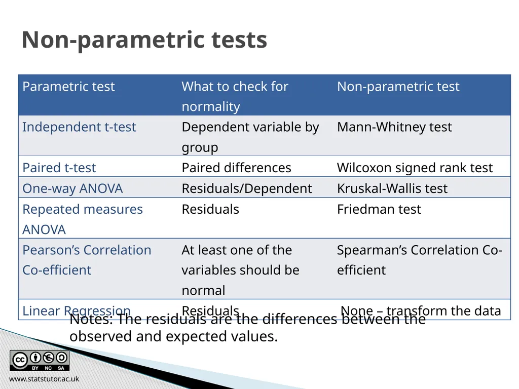
Parametric or non-parametric? Statistical tests fall into two types:

Parametric tests

Non-parametric Assume data follows a particular distribution e.g. normal Nonparametric techniques are usually based on ranks/ signs rather than actual data www.statstutor.ac.uk

141

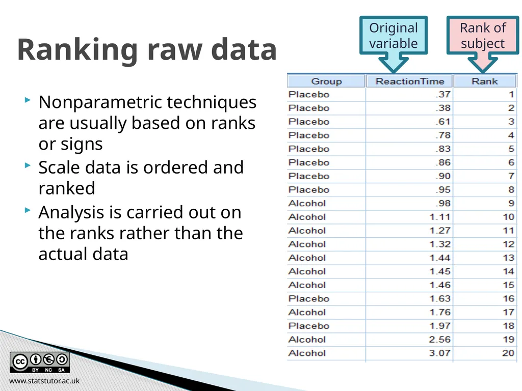
Nonparametric techniques are usually based on ranks or signs
Scale data is ordered and ranked
Analysis is carried out on the ranks rather than the actual data Ranking raw data Original variable Rank of subject www.statstutor.ac.uk

142

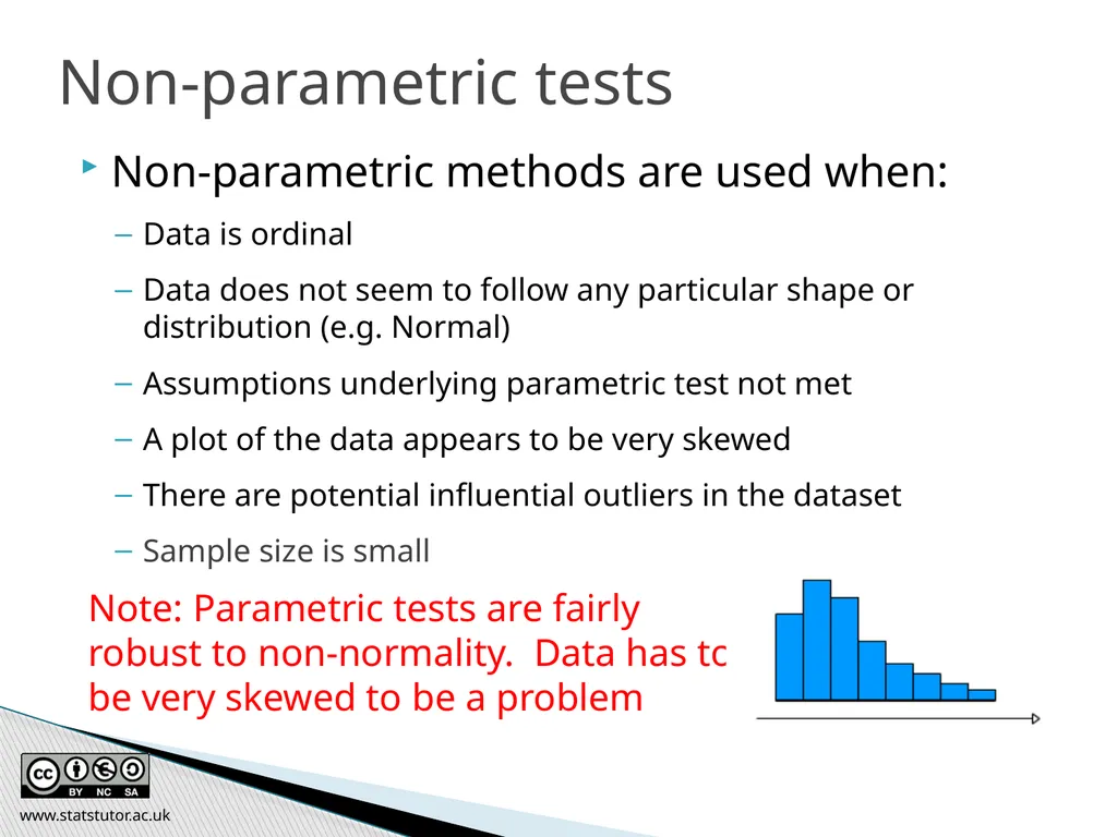
Non-parametric tests Non-parametric methods are used when:
Data is ordinal
Data does not seem to follow any particular shape or distribution (e.g. Normal)
Assumptions underlying parametric test not met
A plot of the data appears to be very skewed
There are potential influential outliers in the dataset
Sample size is small Note: Parametric tests are fairly robust to non-normality. Data has to be very skewed to be a problem www.statstutor.ac.uk

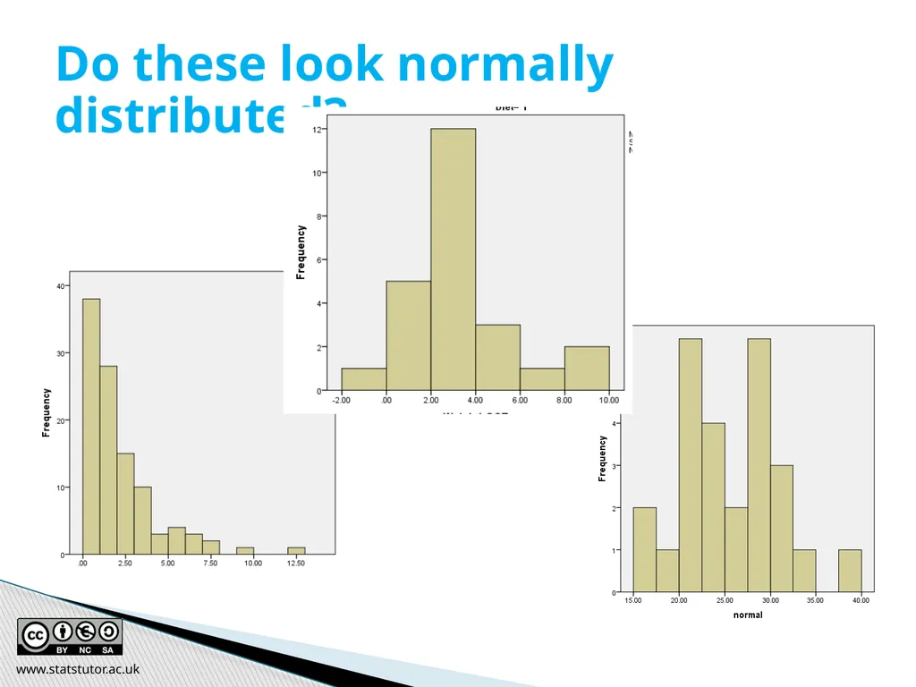
143

Do these look normally distributed? www.statstutor.ac.uk

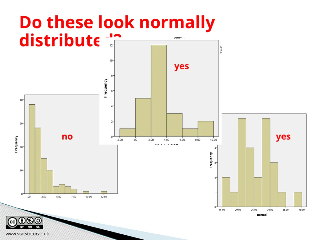
144

Do these look normally distributed? www.statstutor.ac.uk yes yes no

145

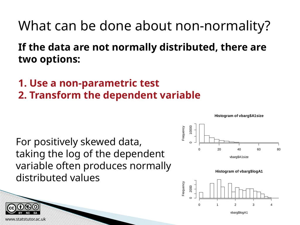
What can be done about non-normality? For positively skewed data, taking the log of the dependent variable often produces normally distributed values If the data are not normally distributed, there are two options:

Use a non-parametric test
Transform the dependent variable www.statstutor.ac.uk

146

Non-parametric tests Notes: The residuals are the differences between the observed and expected values. www.statstutor.ac.uk

147

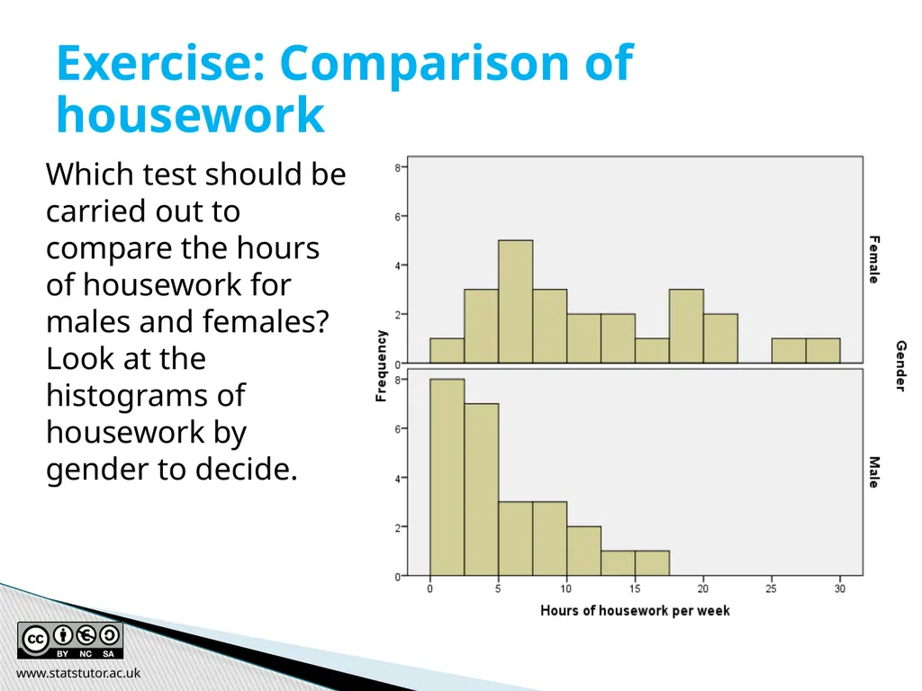
Which test should be carried out to compare the hours of housework for males and females? Look at the histograms of housework by gender to decide. Exercise: Comparison of housework www.statstutor.ac.uk

148

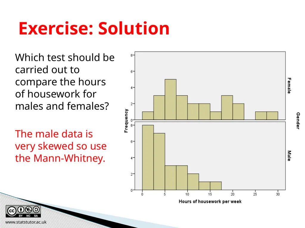
Which test should be carried out to compare the hours of housework for males and females?

The male data is very skewed so use the Mann-Whitney. Exercise: Solution www.statstutor.ac.uk

149

Summary www.statstutor.ac.uk

150

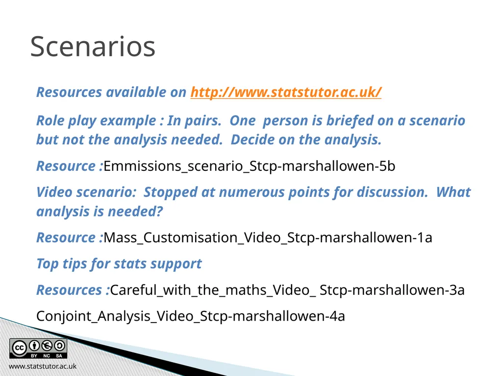
Scenarios Resources available on http://www.statstutor.ac.uk/
Role play example : In pairs. One person is briefed on a scenario but not the analysis needed. Decide on the analysis.
Resource :Emmissions_scenario_Stcp-marshallowen-5b
Video scenario: Stopped at numerous points for discussion. What analysis is needed?
Resource :Mass_Customisation_Video_Stcp-marshallowen-1a
Top tips for stats support
Resources :Careful_with_the_maths_Video_ Stcp-marshallowen-3a
Conjoint_Analysis_Video_Stcp-marshallowen-4a www.statstutor.ac.uk

151

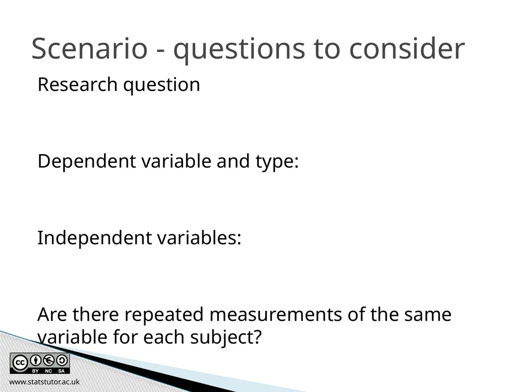
Scenario - questions to consider Research question

Dependent variable and type:

Independent variables:

Are there repeated measurements of the same variable for each subject? www.statstutor.ac.uk

152

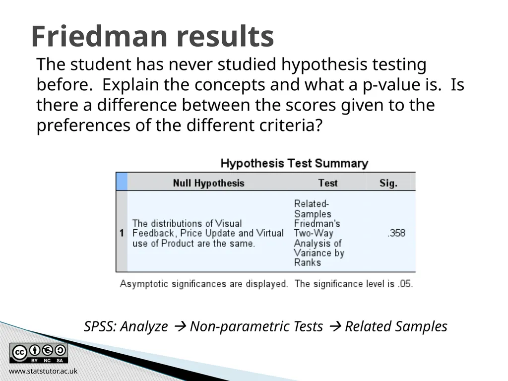
The student has never studied hypothesis testing before. Explain the concepts and what a p-value is. Is there a difference between the scores given to the preferences of the different criteria? Friedman results SPSS: Analyze  Non-parametric Tests  Related Samples www.statstutor.ac.uk

153

Do you feel that you
Have improved your ability to recall and describe some basic applied statistical methods?

Have developed ideas for explaining some of these methods to students in a maths support setting?

Feel more confident about providing statistics support with the topics covered? Resume www.statstutor.ac.uk

154

Additional material www.statstutor.ac.uk Ellen Marshall / Alun Owen
University of Sheffield / University of Worcester Reviewer: Ruth Fairclough
University of Wolverhampton community project
encouraging academics to share statistics support resources
All stcp resources are released under a Creative Commons licence

155

Mann Whitney Test www.statstutor.ac.uk Ellen Marshall / Alun Owen
University of Sheffield / University of Worcester Reviewer: Ruth Fairclough
University of Wolverhampton community project
encouraging academics to share statistics support resources
All stcp resources are released under a Creative Commons licence

156

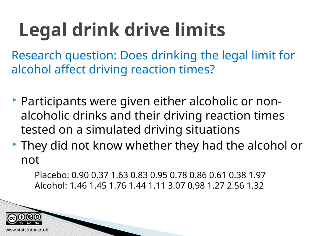
Research question: Does drinking the legal limit for alcohol affect driving reaction times?

Participants were given either alcoholic or non-alcoholic drinks and their driving reaction times tested on a simulated driving situations
They did not know whether they had the alcohol or not Legal drink drive limits Placebo: 0.90 0.37 1.63 0.83 0.95 0.78 0.86 0.61 0.38 1.97
Alcohol: 1.46 1.45 1.76 1.44 1.11 3.07 0.98 1.27 2.56 1.32 www.statstutor.ac.uk

157

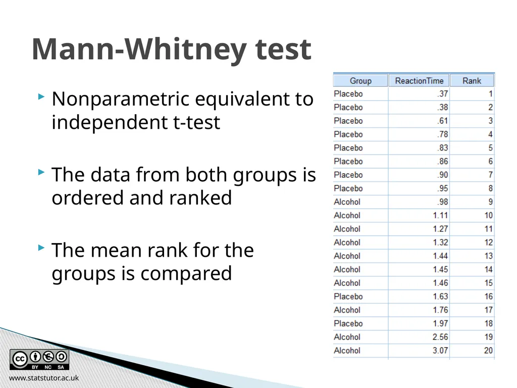
Nonparametric equivalent to independent t-test

The data from both groups is ordered and ranked

The mean rank for the groups is compared Mann-Whitney test www.statstutor.ac.uk

158

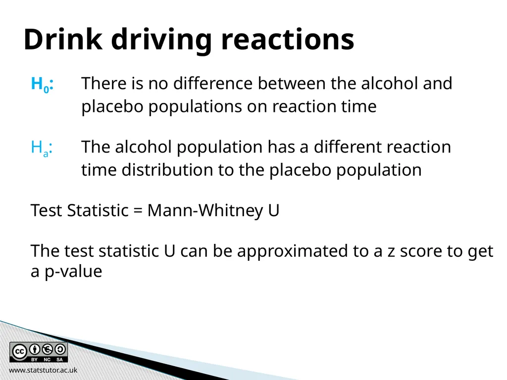
Drink driving reactions H0: There is no difference between the alcohol and
placebo populations on reaction time

Ha: The alcohol population has a different reaction
time distribution to the placebo population

Test Statistic = Mann-Whitney U

The test statistic U can be approximated to a z score to get a p-value www.statstutor.ac.uk

159

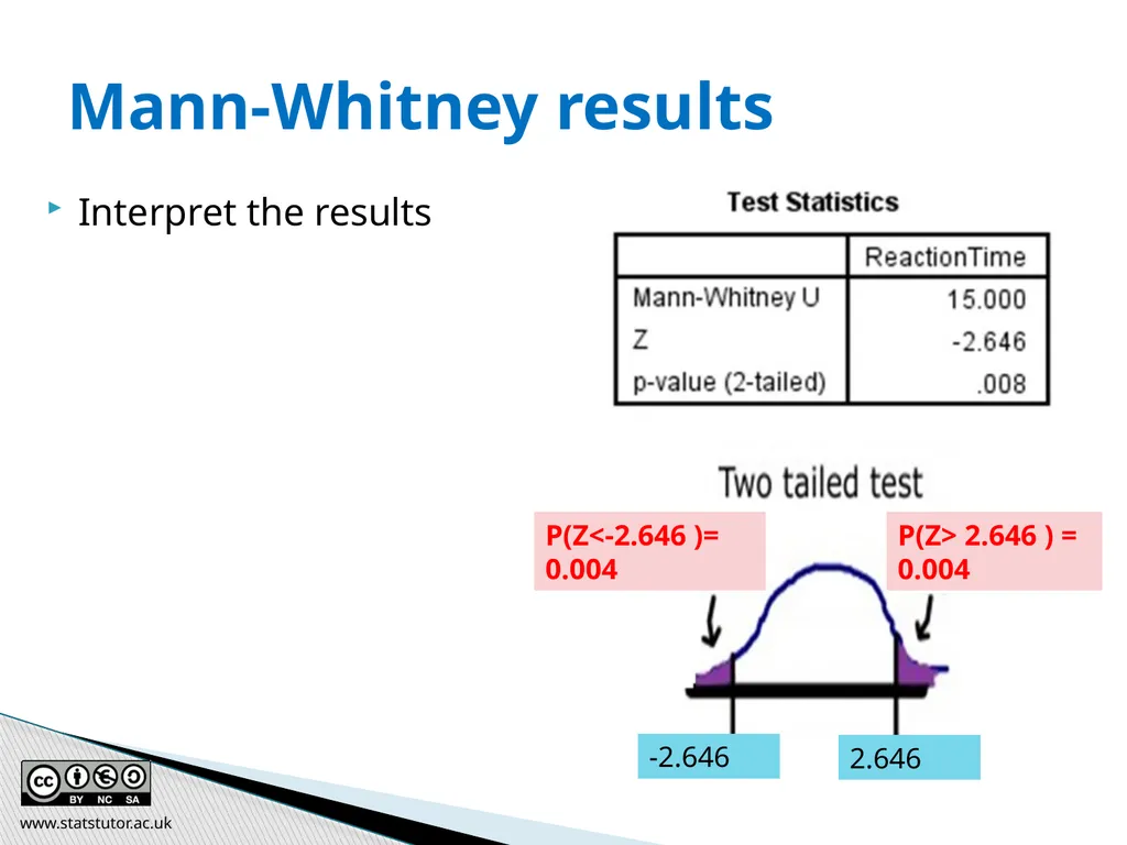
Interpret the results Mann-Whitney results 2.646 www.statstutor.ac.uk

160

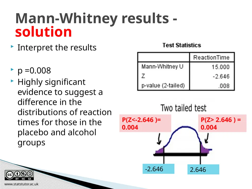
Interpret the results

p =0.008
Highly significant evidence to suggest a difference in the distributions of reaction times for those in the placebo and alcohol groups Mann-Whitney results - solution 2.646 www.statstutor.ac.uk

161

ANOVA www.statstutor.ac.uk Ellen Marshall / Alun Owen
University of Sheffield / University of Worcester Reviewer: Ruth Fairclough
University of Wolverhampton community project
encouraging academics to share statistics support resources
All stcp resources are released under a Creative Commons licence

162

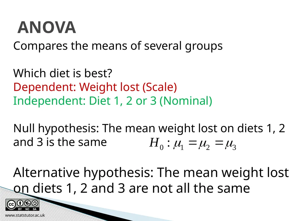
Compares the means of several groups

Which diet is best?
Dependent: Weight lost (Scale)
Independent: Diet 1, 2 or 3 (Nominal)

Null hypothesis: The mean weight lost on diets 1, 2 and 3 is the same

Alternative hypothesis: The mean weight lost on diets 1, 2 and 3 are not all the same ANOVA www.statstutor.ac.uk

163

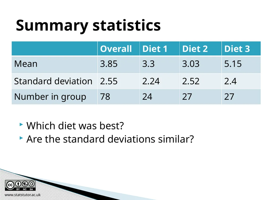
Which diet was best?
Are the standard deviations similar? Summary statistics www.statstutor.ac.uk

164

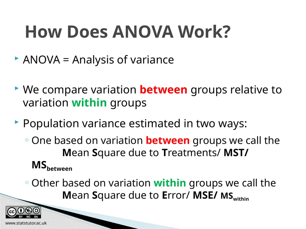
How Does ANOVA Work? ANOVA = Analysis of variance

We compare variation between groups relative to variation within groups

Population variance estimated in two ways:
One based on variation between groups we call the Mean Square due to Treatments/ MST/ MSbetween
Other based on variation within groups we call the Mean Square due to Error/ MSE/ MSwithin www.statstutor.ac.uk

165

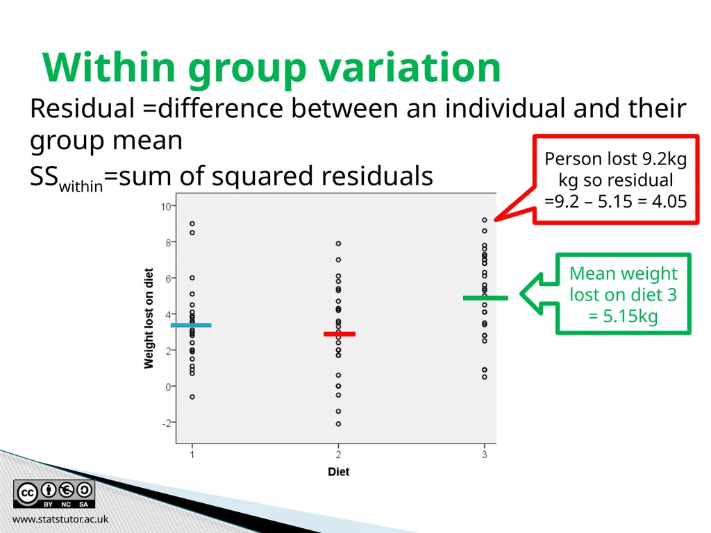
Residual =difference between an individual and their group mean
SSwithin=sum of squared residuals Within group variation Mean weight lost on diet 3 = 5.15kg Person lost 9.2kg kg so residual =9.2 – 5.15 = 4.05 www.statstutor.ac.uk

166

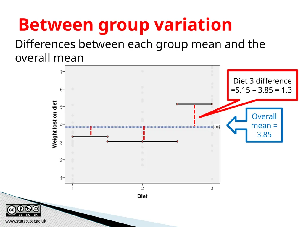
Differences between each group mean and the overall mean Between group variation www.statstutor.ac.uk

167

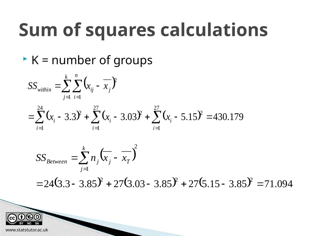
K = number of groups Sum of squares calculations www.statstutor.ac.uk

168

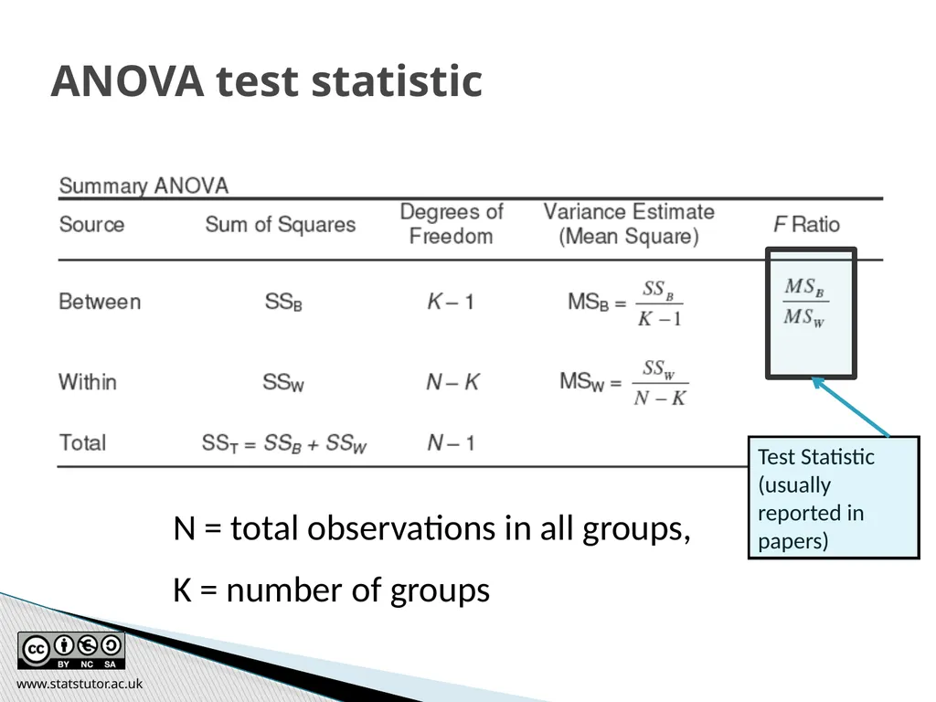
N = total observations in all groups,
K = number of groups Test Statistic (usually reported in papers) ANOVA test statistic www.statstutor.ac.uk

169

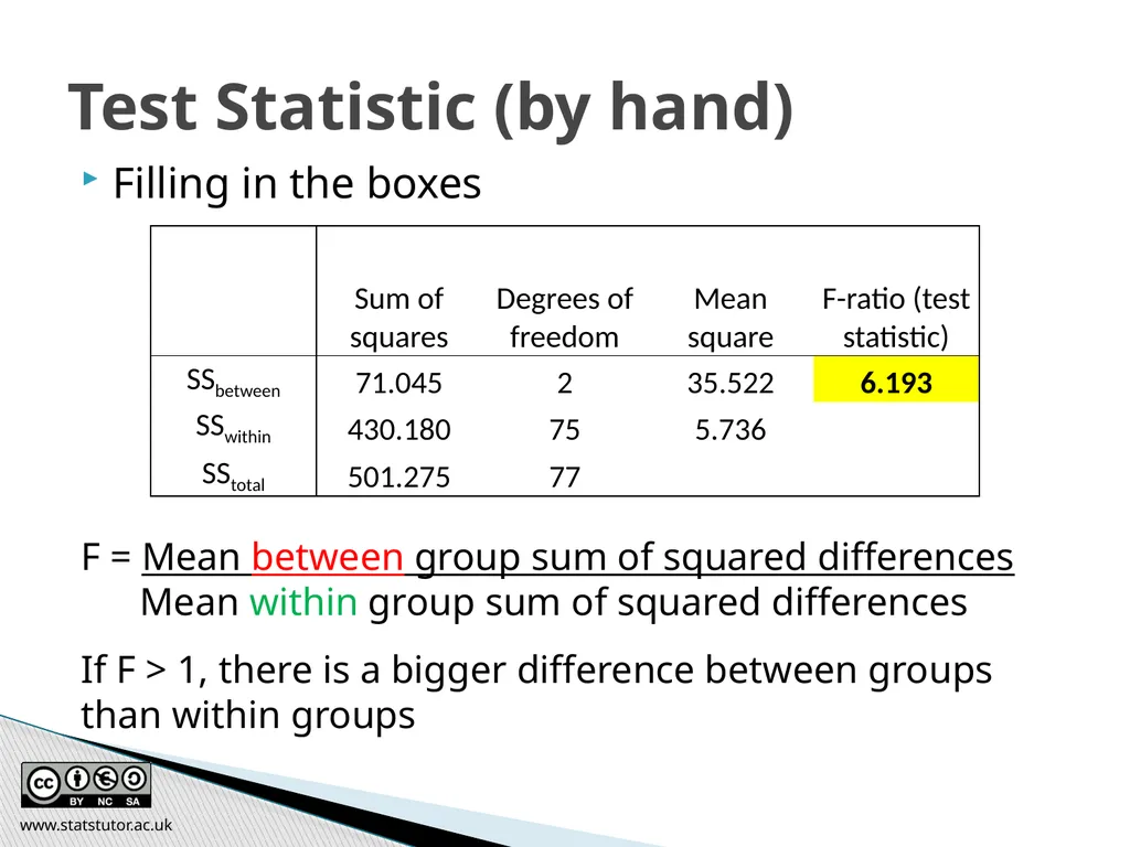
Filling in the boxes Test Statistic (by hand) F = Mean between group sum of squared differences
Mean within group sum of squared differences

If F > 1, there is a bigger difference between groups than within groups www.statstutor.ac.uk

170

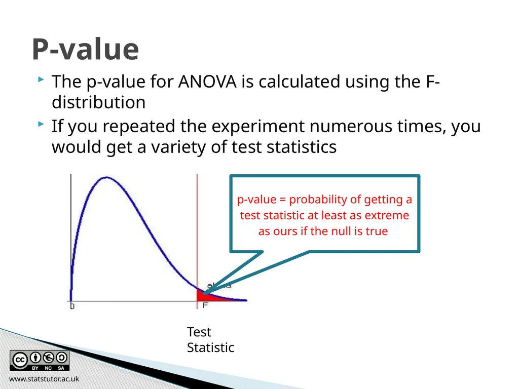
The p-value for ANOVA is calculated using the F-distribution
If you repeated the experiment numerous times, you would get a variety of test statistics P-value p-value = probability of getting a test statistic at least as extreme as ours if the null is true Test Statistic www.statstutor.ac.uk

171

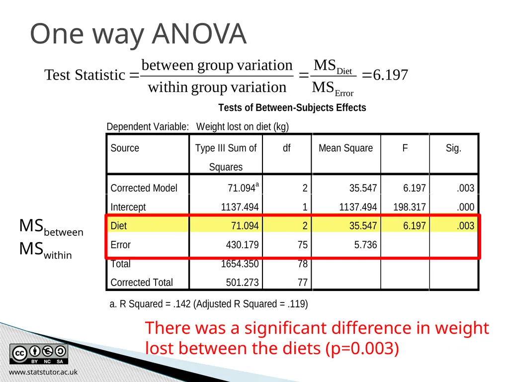
One way ANOVA There was a significant difference in weight lost between the diets (p=0.003) MSbetween
MSwithin www.statstutor.ac.uk

172

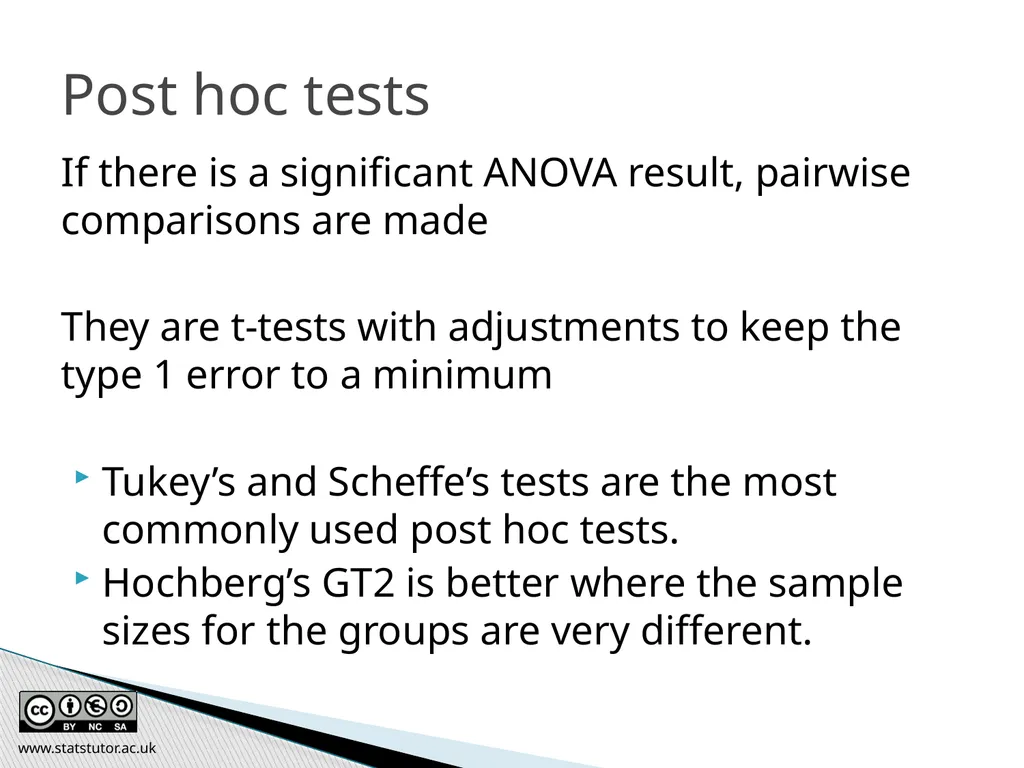
Post hoc tests If there is a significant ANOVA result, pairwise comparisons are made

They are t-tests with adjustments to keep the type 1 error to a minimum

Tukey’s and Scheffe’s tests are the most commonly used post hoc tests.
Hochberg’s GT2 is better where the sample sizes for the groups are very different. www.statstutor.ac.uk

173

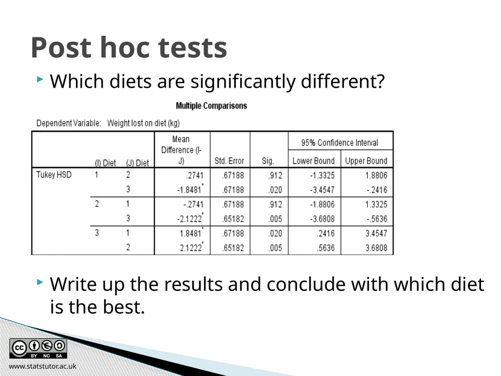
Which diets are significantly different?

Write up the results and conclude with which diet is the best. Post hoc tests www.statstutor.ac.uk

174

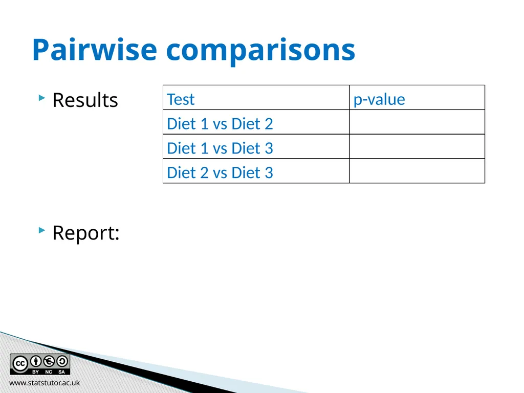
Results

Report: Pairwise comparisons www.statstutor.ac.uk

175

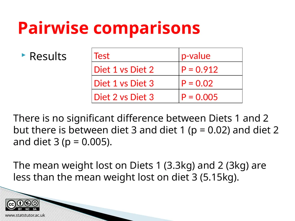
Results Pairwise comparisons There is no significant difference between Diets 1 and 2 but there is between diet 3 and diet 1 (p = 0.02) and diet 2 and diet 3 (p = 0.005).

The mean weight lost on Diets 1 (3.3kg) and 2 (3kg) are less than the mean weight lost on diet 3 (5.15kg). www.statstutor.ac.uk

176

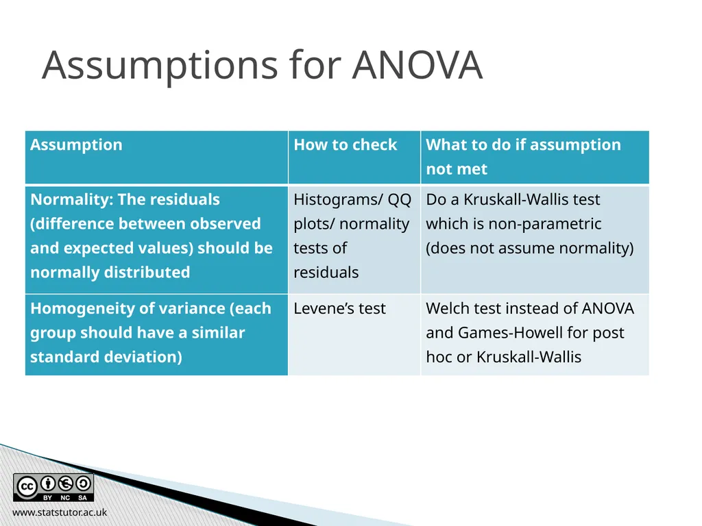
Assumptions for ANOVA www.statstutor.ac.uk

177

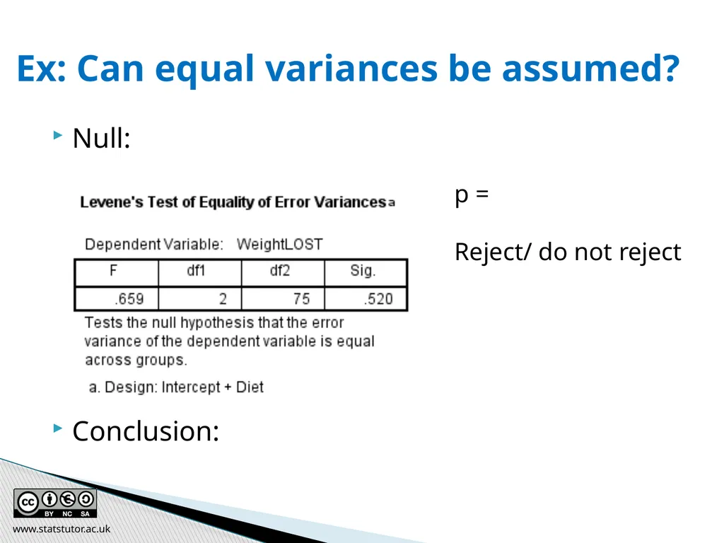
Null:

Conclusion: Ex: Can equal variances be assumed? p =

Reject/ do not reject www.statstutor.ac.uk

178

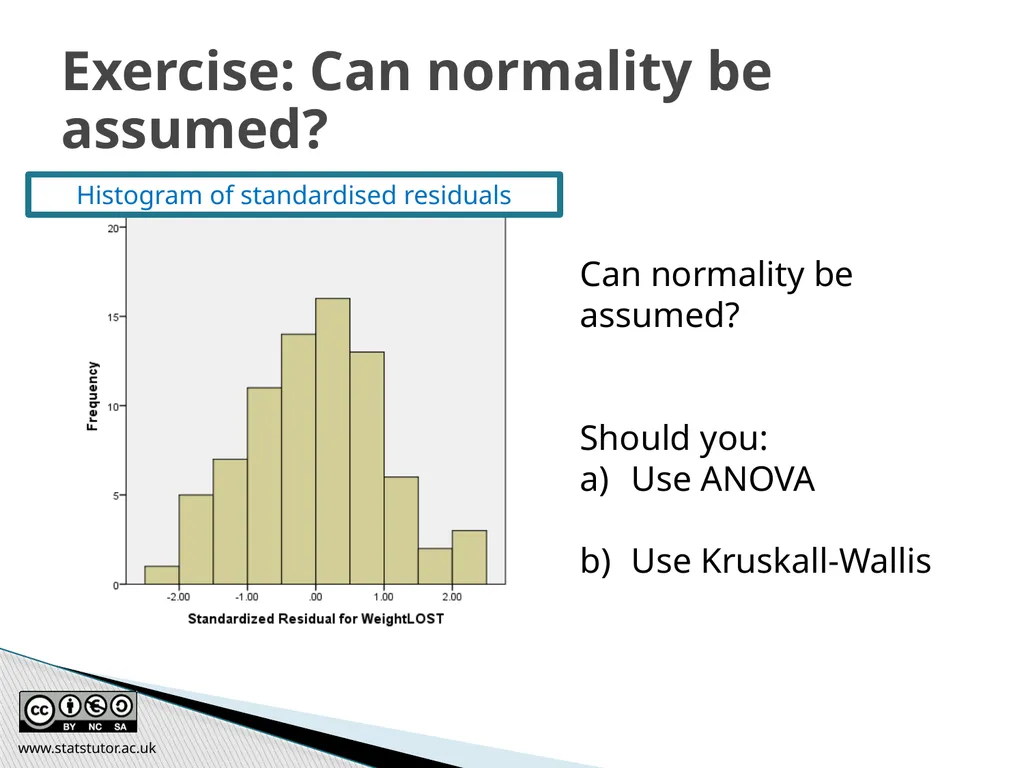
Conclusion: Exercise: Can normality be assumed? Can normality be assumed?

Should you:
Use ANOVA

Use Kruskall-Wallis Histogram of standardised residuals www.statstutor.ac.uk

179

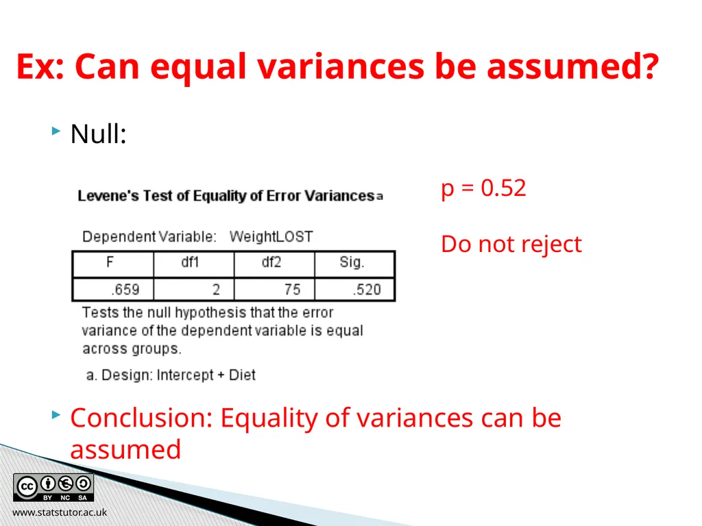
Null:

Conclusion: Equality of variances can be assumed Ex: Can equal variances be assumed? p = 0.52

Do not reject www.statstutor.ac.uk

180

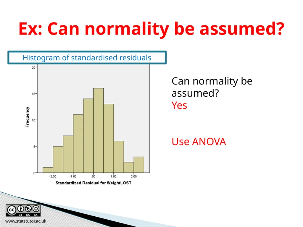
Conclusion: Ex: Can normality be assumed? Can normality be assumed?
Yes

Use ANOVA Histogram of standardised residuals www.statstutor.ac.uk

181

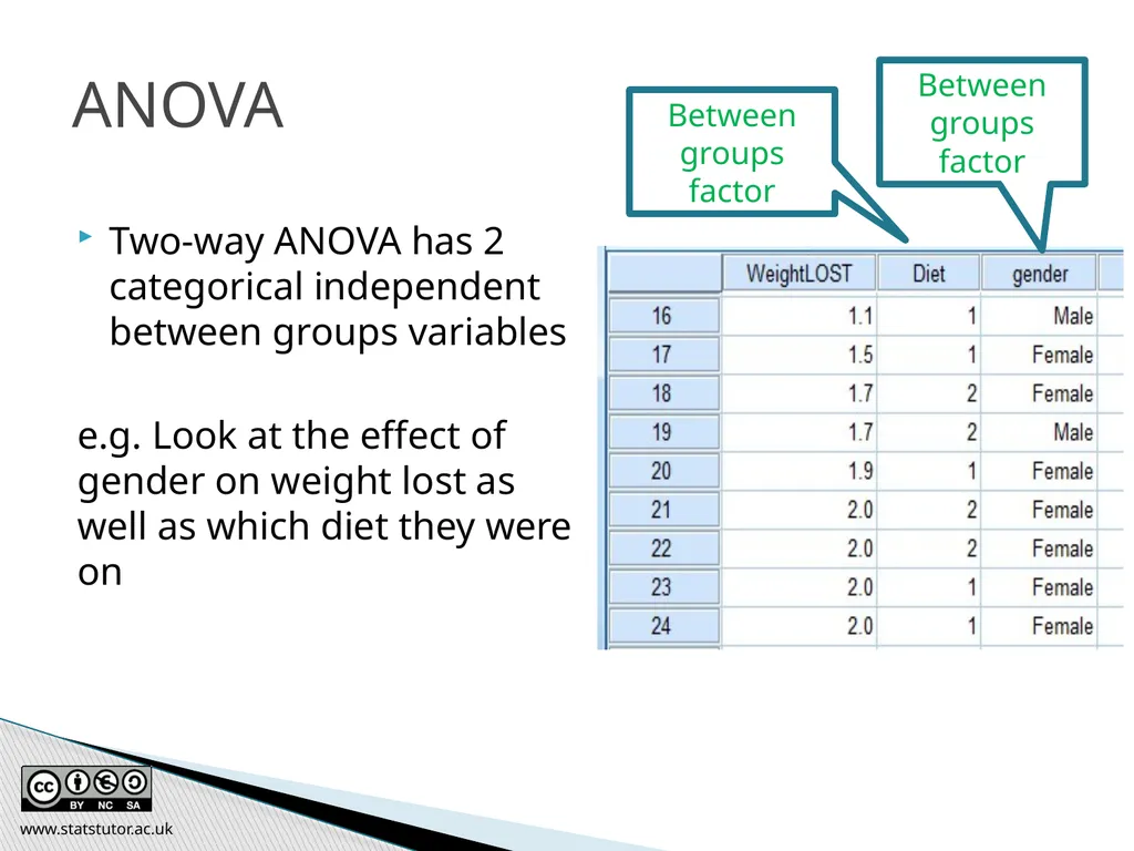
ANOVA Two-way ANOVA has 2 categorical independent between groups variables

e.g. Look at the effect of gender on weight lost as well as which diet they were on Between groups factor Between groups factor www.statstutor.ac.uk

182

Dependent = Weight Lost
Independents: Diet and Gender

Tests 3 hypotheses:
Mean weight loss does not differ by diet
Mean weight loss does not differ by gender
There is no interaction between diet and gender

What’s an interaction? Two-way ANOVA www.statstutor.ac.uk

183

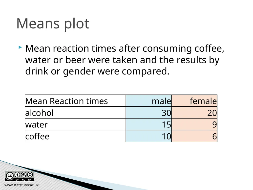
Means plot Mean reaction times after consuming coffee, water or beer were taken and the results by drink or gender were compared. www.statstutor.ac.uk

184

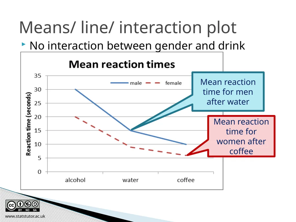
Means/ line/ interaction plot No interaction between gender and drink Mean reaction time for men after water Mean reaction time for women after coffee www.statstutor.ac.uk

185

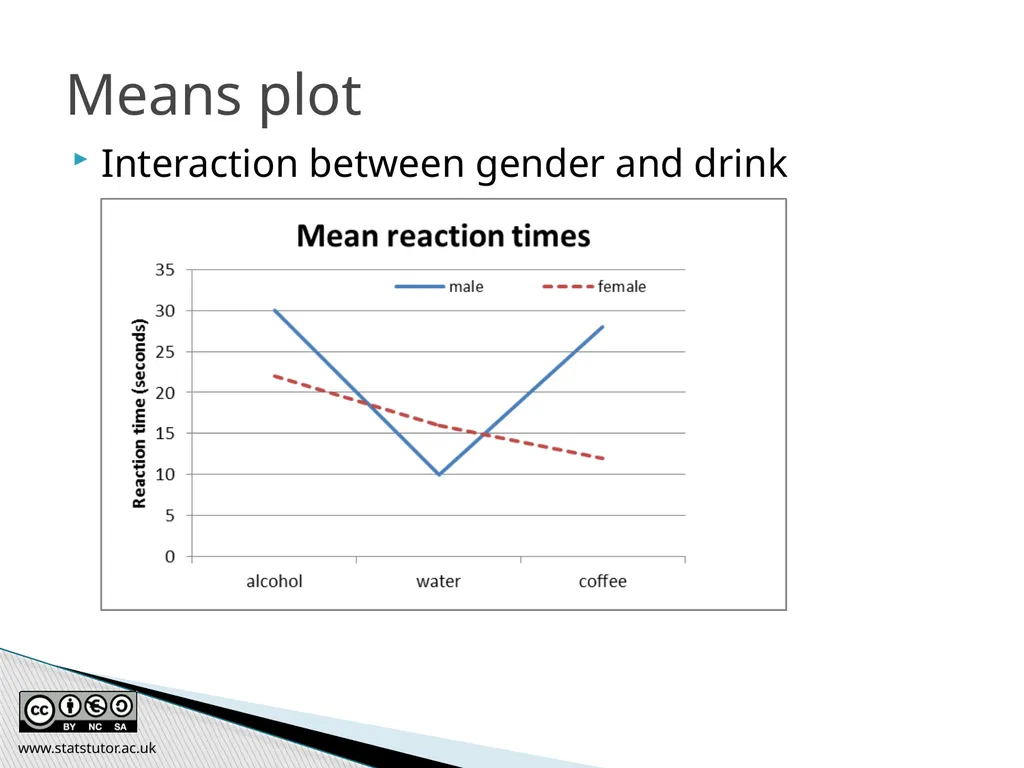
Means plot Interaction between gender and drink www.statstutor.ac.uk

186

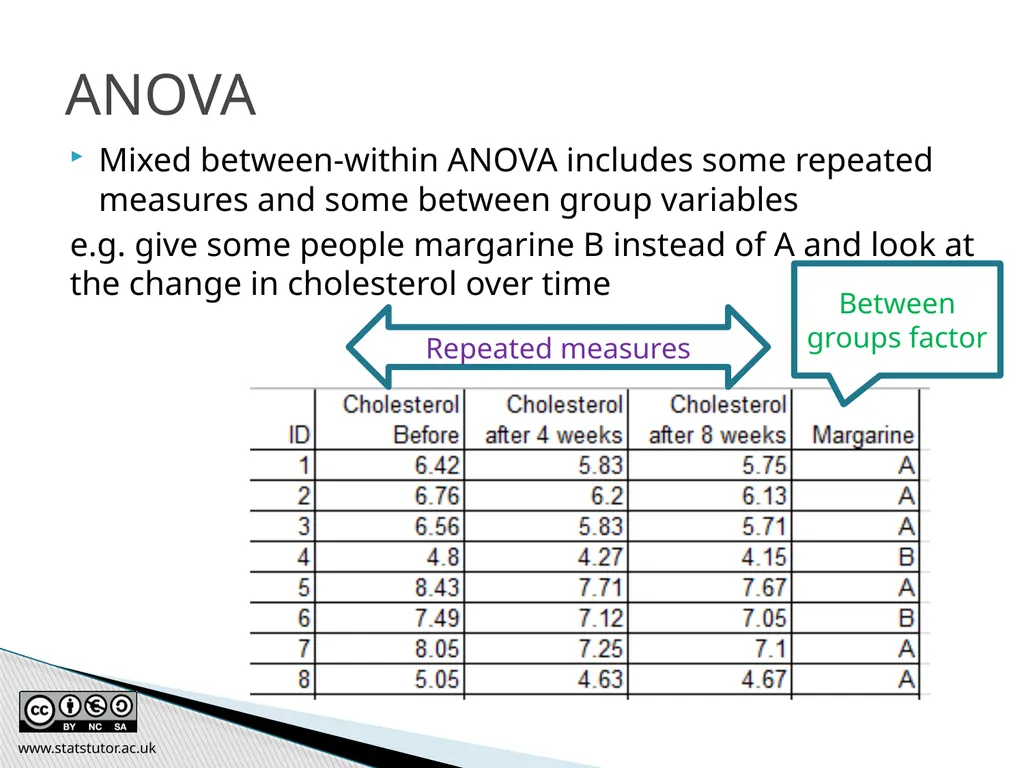
ANOVA Mixed between-within ANOVA includes some repeated measures and some between group variables
e.g. give some people margarine B instead of A and look at the change in cholesterol over time Repeated measures Between groups factor www.statstutor.ac.uk

Introductory Statistics and Hypothesis Testing

Related Topics

Download this presentation From Below

Presentation Transcript

Introductory Statistics and Hypothesis Testing

Related Topics

Share

Embed code

Download this presentation From Below

Presentation Transcript