
Lecture 3 Part 1.Important Database Concepts Part
MS
Published · 68 slides · 0 views
1 / 1
Description
Lecture 3 Part 1.Important Database Concepts Part 2. Queries People typically use a number system with base 10 each digit corresponds to 10 to some power a number with 3 digits has 103 or 1000 possibilities Computer use a base 8 system of
Related Topics
Share
Embed code
Download this presentation From Below
"Lecture 3 Part 1.Important Database Concepts Part" is the property of its rightful owner. Permission is granted to download and print the materials on this website for personal, non-commercial use only, and to display it on your personal computer provided you do not modify the materials and that you retain all copyright notices contained in the materials. By downloading content from our website, you accept the terms of this agreement.
Presentation Transcript
01
Lecture 3
Part 1.Important Database Concepts
Part 2. Queries<br>
Part 1.Important Database Concepts
Part 2. Queries<br>
02
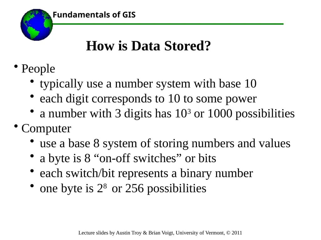
People
typically use a number system with base 10
each digit corresponds to 10 to some power
a number with 3 digits has 103 or 1000 possibilities
Computer
use a base 8 system of storing numbers and values
a byte is 8 “on-off switches” or bits
each switch/bit represents a binary number
one byte is 28 or 256 possibilities How is Data Stored?<br>
typically use a number system with base 10
each digit corresponds to 10 to some power
a number with 3 digits has 103 or 1000 possibilities
Computer
use a base 8 system of storing numbers and values
a byte is 8 “on-off switches” or bits
each switch/bit represents a binary number
one byte is 28 or 256 possibilities How is Data Stored?<br>
03
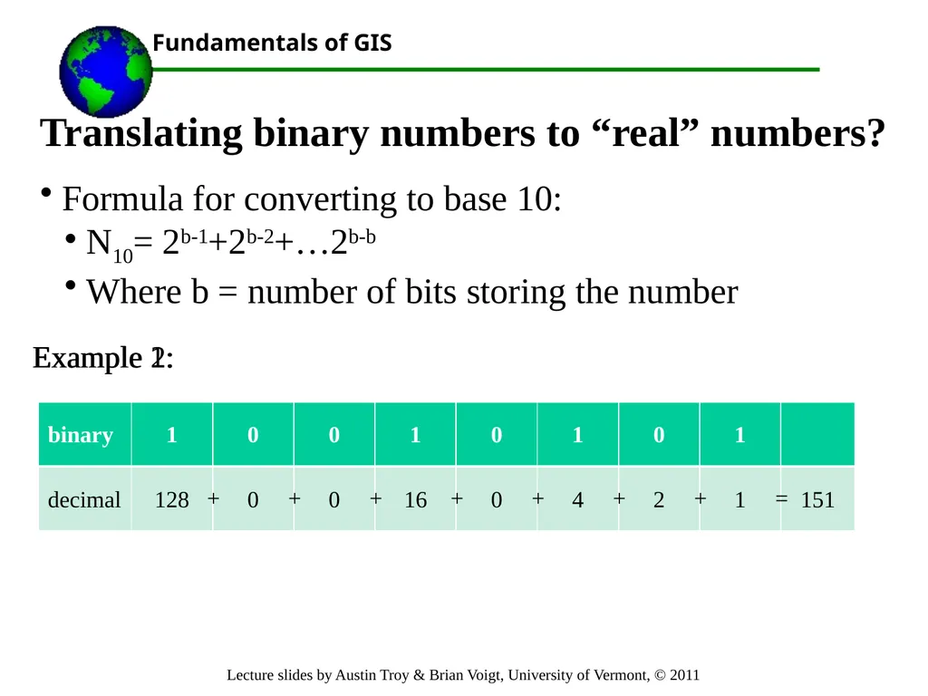
Formula for converting to base 10:
N10= 2b-1+2b-2+…2b-b
Where b = number of bits storing the number Translating binary numbers to “real” numbers? Example 1: Example 2:<br>
N10= 2b-1+2b-2+…2b-b
Where b = number of bits storing the number Translating binary numbers to “real” numbers? Example 1: Example 2:<br>
04
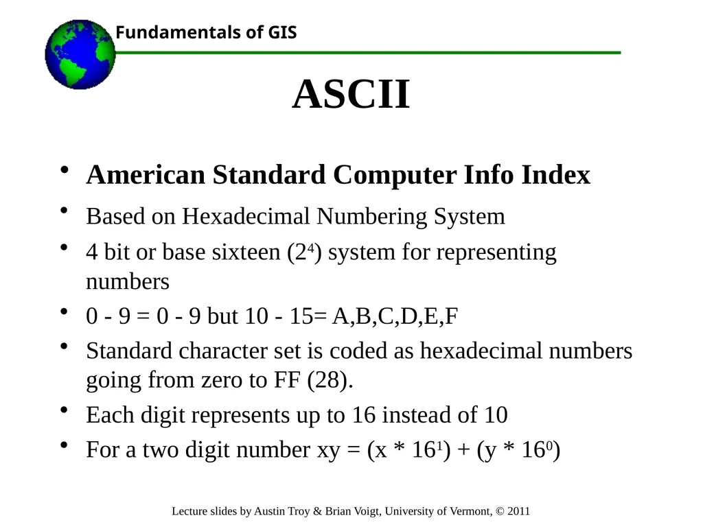
ASCII American Standard Computer Info Index
Based on Hexadecimal Numbering System
4 bit or base sixteen (24) system for representing numbers
0 - 9 = 0 - 9 but 10 - 15= A,B,C,D,E,F
Standard character set is coded as hexadecimal numbers going from zero to FF (28).
Each digit represents up to 16 instead of 10
For a two digit number xy = (x * 161) + (y * 160)<br>
Based on Hexadecimal Numbering System
4 bit or base sixteen (24) system for representing numbers
0 - 9 = 0 - 9 but 10 - 15= A,B,C,D,E,F
Standard character set is coded as hexadecimal numbers going from zero to FF (28).
Each digit represents up to 16 instead of 10
For a two digit number xy = (x * 161) + (y * 160)<br>
05
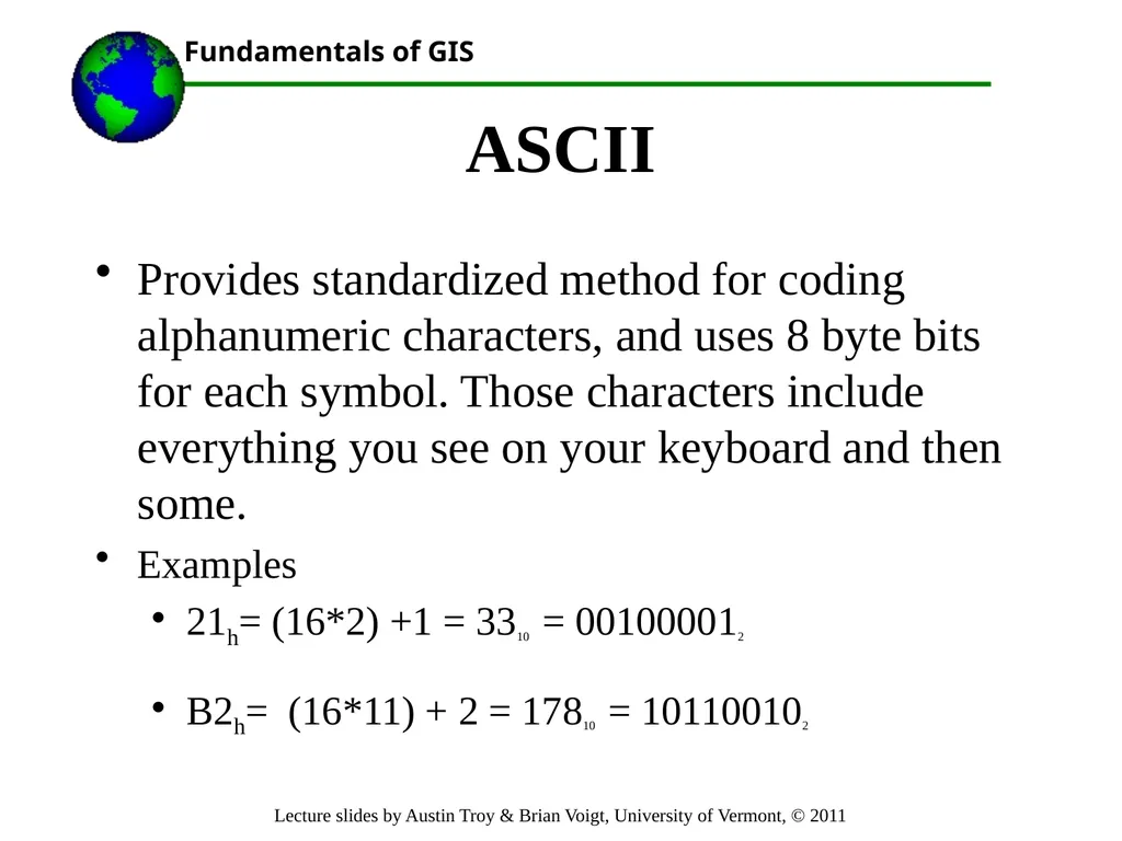
ASCII Provides standardized method for coding alphanumeric characters, and uses 8 byte bits for each symbol. Those characters include everything you see on your keyboard and then some.
Examples
21h= (16*2) +1 = 3310 = 001000012
B2h= (16*11) + 2 = 17810 = 101100102<br>
Examples
21h= (16*2) +1 = 3310 = 001000012
B2h= (16*11) + 2 = 17810 = 101100102<br>
06
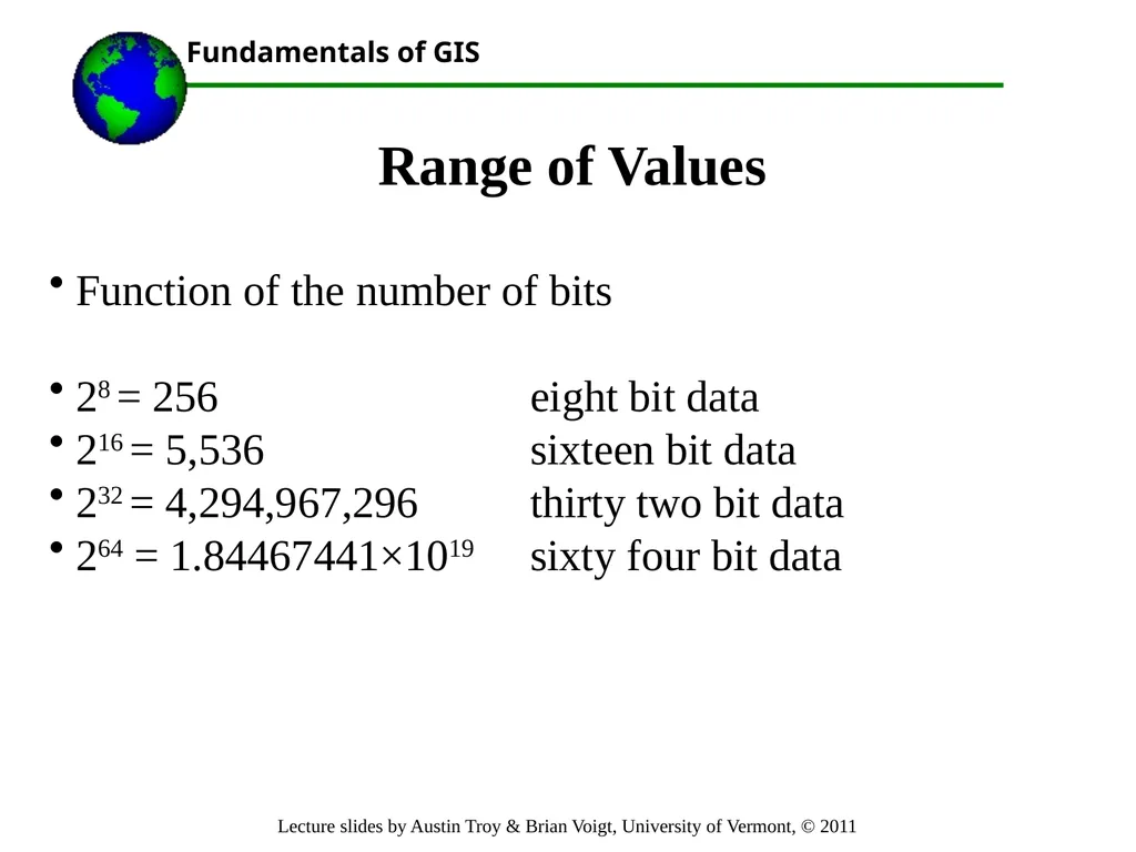
Function of the number of bits
28 = 256 eight bit data
216 = 5,536 sixteen bit data
232 = 4,294,967,296 thirty two bit data
264 = 1.84467441×10¹⁹ sixty four bit data Range of Values<br>
28 = 256 eight bit data
216 = 5,536 sixteen bit data
232 = 4,294,967,296 thirty two bit data
264 = 1.84467441×10¹⁹ sixty four bit data Range of Values<br>
07
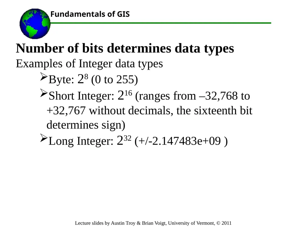
Number of bits determines data types
Examples of Integer data types
Byte: 28 (0 to 255)
Short Integer: 216 (ranges from –32,768 to +32,767 without decimals, the sixteenth bit determines sign)
Long Integer: 232 (+/-2.147483e+09 )<br>
Examples of Integer data types
Byte: 28 (0 to 255)
Short Integer: 216 (ranges from –32,768 to +32,767 without decimals, the sixteenth bit determines sign)
Long Integer: 232 (+/-2.147483e+09 )<br>
08
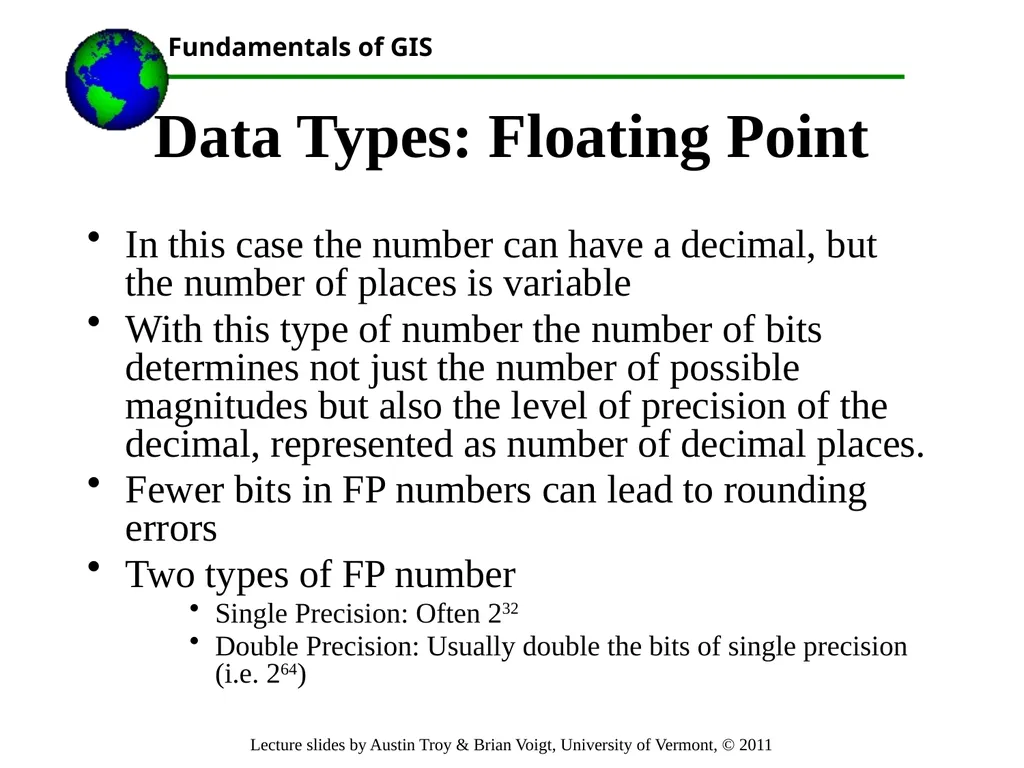
Data Types: Floating Point In this case the number can have a decimal, but the number of places is variable
With this type of number the number of bits determines not just the number of possible magnitudes but also the level of precision of the decimal, represented as number of decimal places.
Fewer bits in FP numbers can lead to rounding errors
Two types of FP number
Single Precision: Often 232
Double Precision: Usually double the bits of single precision (i.e. 264)<br>
With this type of number the number of bits determines not just the number of possible magnitudes but also the level of precision of the decimal, represented as number of decimal places.
Fewer bits in FP numbers can lead to rounding errors
Two types of FP number
Single Precision: Often 232
Double Precision: Usually double the bits of single precision (i.e. 264)<br>
09
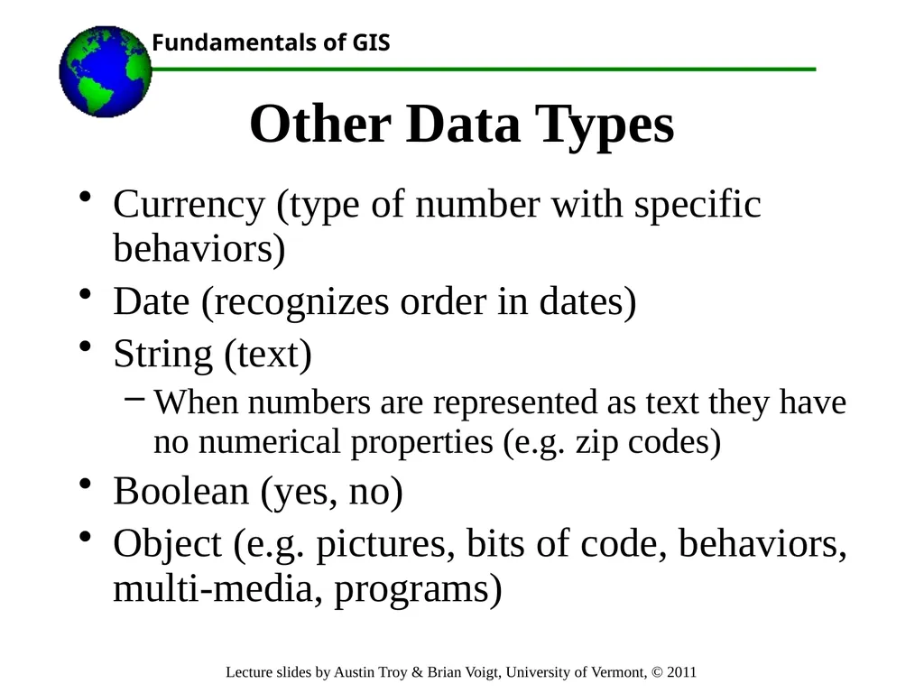
Other Data Types Currency (type of number with specific behaviors)
Date (recognizes order in dates)
String (text)
When numbers are represented as text they have no numerical properties (e.g. zip codes)
Boolean (yes, no)
Object (e.g. pictures, bits of code, behaviors, multi-media, programs)<br>
Date (recognizes order in dates)
String (text)
When numbers are represented as text they have no numerical properties (e.g. zip codes)
Boolean (yes, no)
Object (e.g. pictures, bits of code, behaviors, multi-media, programs)<br>
10
Three database models Hierarchical
Network
Relational<br>
Network
Relational<br>
11
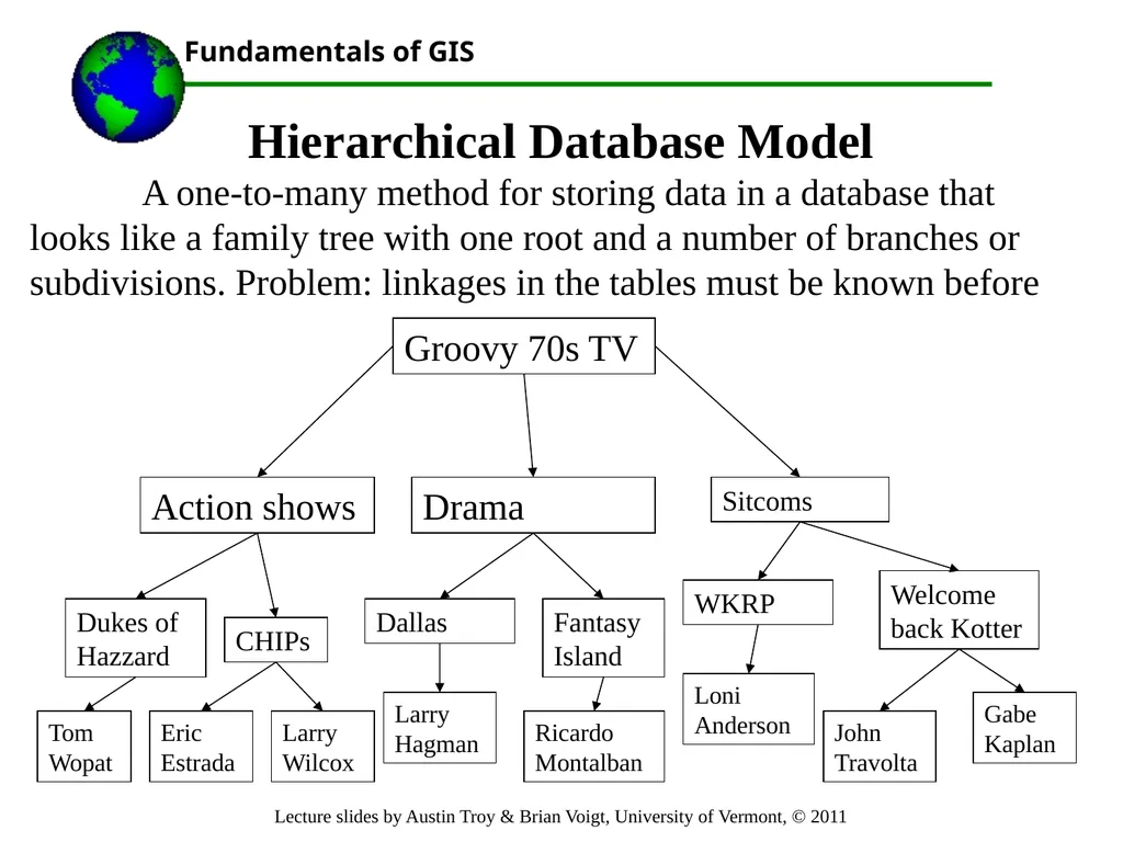
Hierarchical Database Model
A one-to-many method for storing data in a database that looks like a family tree with one root and a number of branches or subdivisions. Problem: linkages in the tables must be known before Groovy 70s TV Action shows Drama Sitcoms Dukes of Hazzard CHIPs Dallas Fantasy Island WKRP Welcome back Kotter Tom Wopat Eric Estrada Gabe Kaplan Loni Anderson Larry Wilcox Larry Hagman Ricardo Montalban John Travolta<br>
A one-to-many method for storing data in a database that looks like a family tree with one root and a number of branches or subdivisions. Problem: linkages in the tables must be known before Groovy 70s TV Action shows Drama Sitcoms Dukes of Hazzard CHIPs Dallas Fantasy Island WKRP Welcome back Kotter Tom Wopat Eric Estrada Gabe Kaplan Loni Anderson Larry Wilcox Larry Hagman Ricardo Montalban John Travolta<br>
12
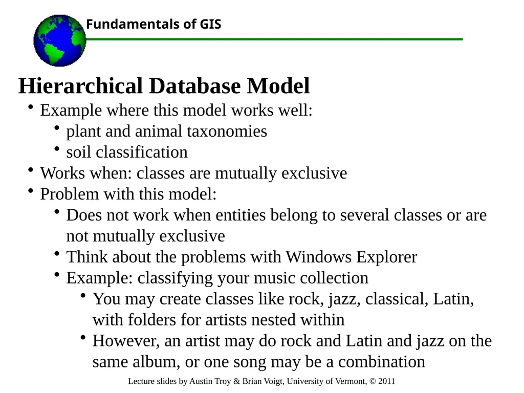
Hierarchical Database Model
Example where this model works well:
plant and animal taxonomies
soil classification
Works when: classes are mutually exclusive
Problem with this model:
Does not work when entities belong to several classes or are not mutually exclusive
Think about the problems with Windows Explorer
Example: classifying your music collection
You may create classes like rock, jazz, classical, Latin, with folders for artists nested within
However, an artist may do rock and Latin and jazz on the same album, or one song may be a combination<br>
Example where this model works well:
plant and animal taxonomies
soil classification
Works when: classes are mutually exclusive
Problem with this model:
Does not work when entities belong to several classes or are not mutually exclusive
Think about the problems with Windows Explorer
Example: classifying your music collection
You may create classes like rock, jazz, classical, Latin, with folders for artists nested within
However, an artist may do rock and Latin and jazz on the same album, or one song may be a combination<br>
13
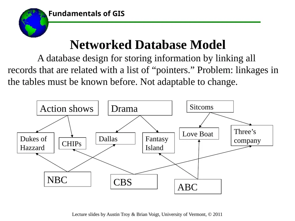
Networked Database Model
A database design for storing information by linking all records that are related with a list of “pointers.” Problem: linkages in the tables must be known before. Not adaptable to change. Action shows Drama Sitcoms Dukes of Hazzard CHIPs Dallas Fantasy Island Love Boat Three’s company ABC CBS NBC<br>
A database design for storing information by linking all records that are related with a list of “pointers.” Problem: linkages in the tables must be known before. Not adaptable to change. Action shows Drama Sitcoms Dukes of Hazzard CHIPs Dallas Fantasy Island Love Boat Three’s company ABC CBS NBC<br>
14
Relational (Tabular) Database Model
A design used in database systems in which relationships are created between one or more flat files (or tables) based on the idea
that each pair of tables has a field in common, or “key”. In a relational database, the records are generally different in each table
The advantages: each table can be prepared and maintained separately, tables can remain separate until a query requires connecting, or relating them, relationships can be one to one, one to many or many to one<br>
A design used in database systems in which relationships are created between one or more flat files (or tables) based on the idea
that each pair of tables has a field in common, or “key”. In a relational database, the records are generally different in each table
The advantages: each table can be prepared and maintained separately, tables can remain separate until a query requires connecting, or relating them, relationships can be one to one, one to many or many to one<br>
15
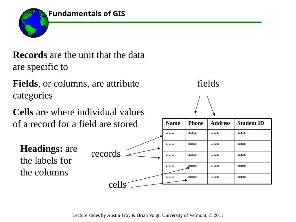
Records are the unit that the data are specific to
Fields, or columns, are attribute categories
Cells are where individual values of a record for a field are stored records fields cells Headings: are the labels for the columns<br>
Fields, or columns, are attribute categories
Cells are where individual values of a record for a field are stored records fields cells Headings: are the labels for the columns<br>
16
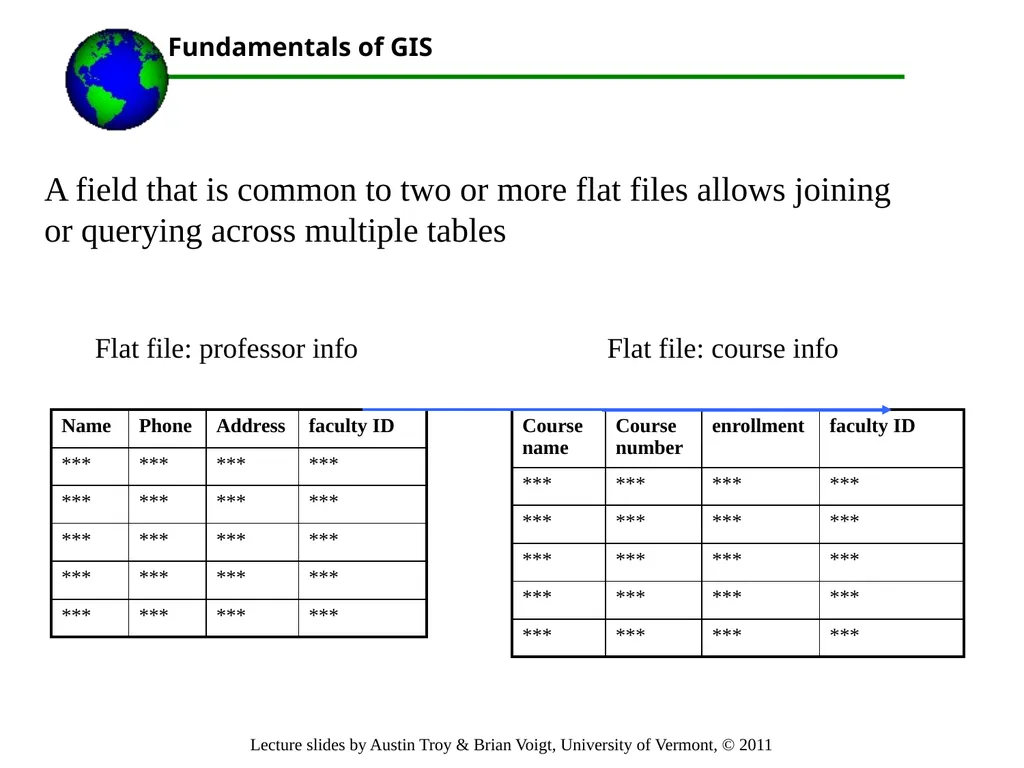
A field that is common to two or more flat files allows joining or querying across multiple tables Flat file: professor info Flat file: course info<br>
17
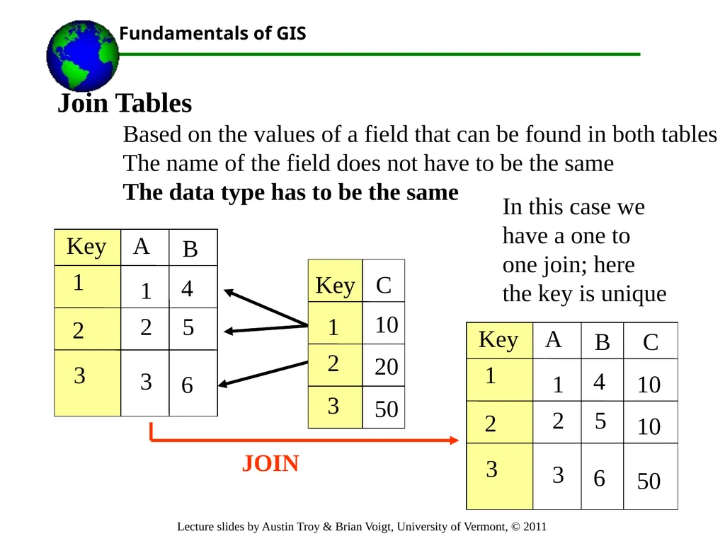
Join Tables
Based on the values of a field that can be found in both tables
The name of the field does not have to be the same
The data type has to be the same Key A B 1 2 3 Key C 1 2 1 2 3 4 5 6 10 20 Key A B 1 2 3 1 2 3 4 5 6 C 10 10 50 JOIN In this case we have a one to one join; here the key is unique 3 50<br>
Based on the values of a field that can be found in both tables
The name of the field does not have to be the same
The data type has to be the same Key A B 1 2 3 Key C 1 2 1 2 3 4 5 6 10 20 Key A B 1 2 3 1 2 3 4 5 6 C 10 10 50 JOIN In this case we have a one to one join; here the key is unique 3 50<br>
18
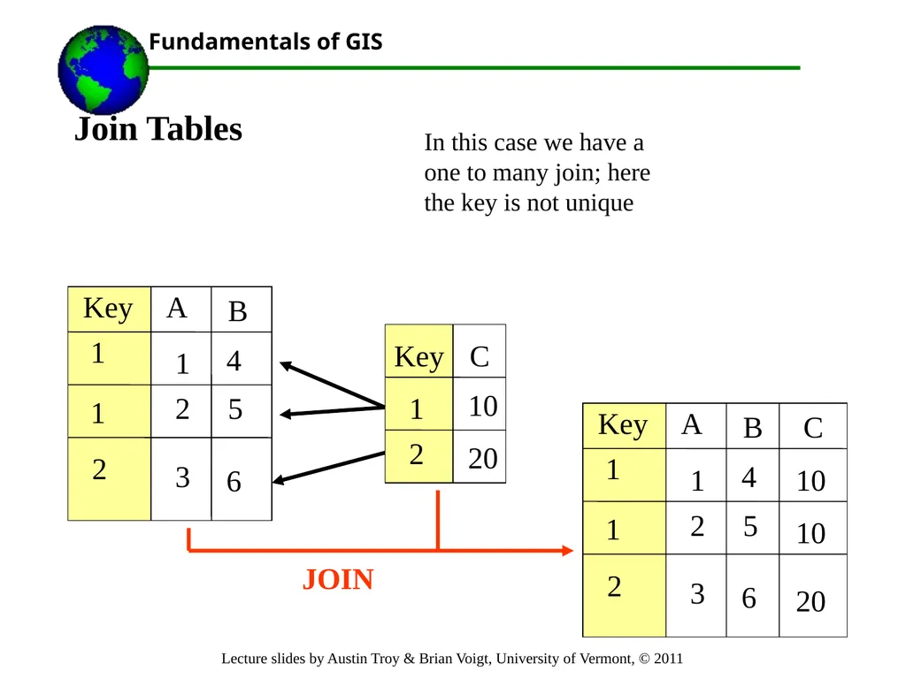
Join Tables Key A B 1 1 2 Key C 1 2 1 2 3 4 5 6 10 20 Key A B 1 1 2 1 2 3 4 5 6 C 10 10 20 JOIN In this case we have a one to many join; here the key is not unique<br>
19
Relational (Tabular) Database Model: 70s TV example
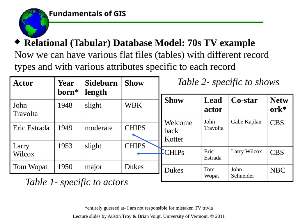
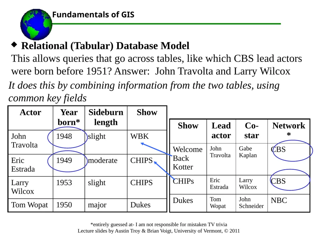
Now we can have various flat files (tables) with different record types and with various attributes specific to each record *entirely guessed at- I am not responsible for mistaken TV trivia Table 1- specific to actors Table 2- specific to shows<br>
Now we can have various flat files (tables) with different record types and with various attributes specific to each record *entirely guessed at- I am not responsible for mistaken TV trivia Table 1- specific to actors Table 2- specific to shows<br>
20
Relational (Tabular) Database Model
This allows queries that go across tables, like which CBS lead actors were born before 1951? Answer: John Travolta and Larry Wilcox *entirely guessed at- I am not responsible for mistaken TV trivia It does this by combining information from the two tables, using common key fields<br>
This allows queries that go across tables, like which CBS lead actors were born before 1951? Answer: John Travolta and Larry Wilcox *entirely guessed at- I am not responsible for mistaken TV trivia It does this by combining information from the two tables, using common key fields<br>
21
Relational (Tabular) Database Model
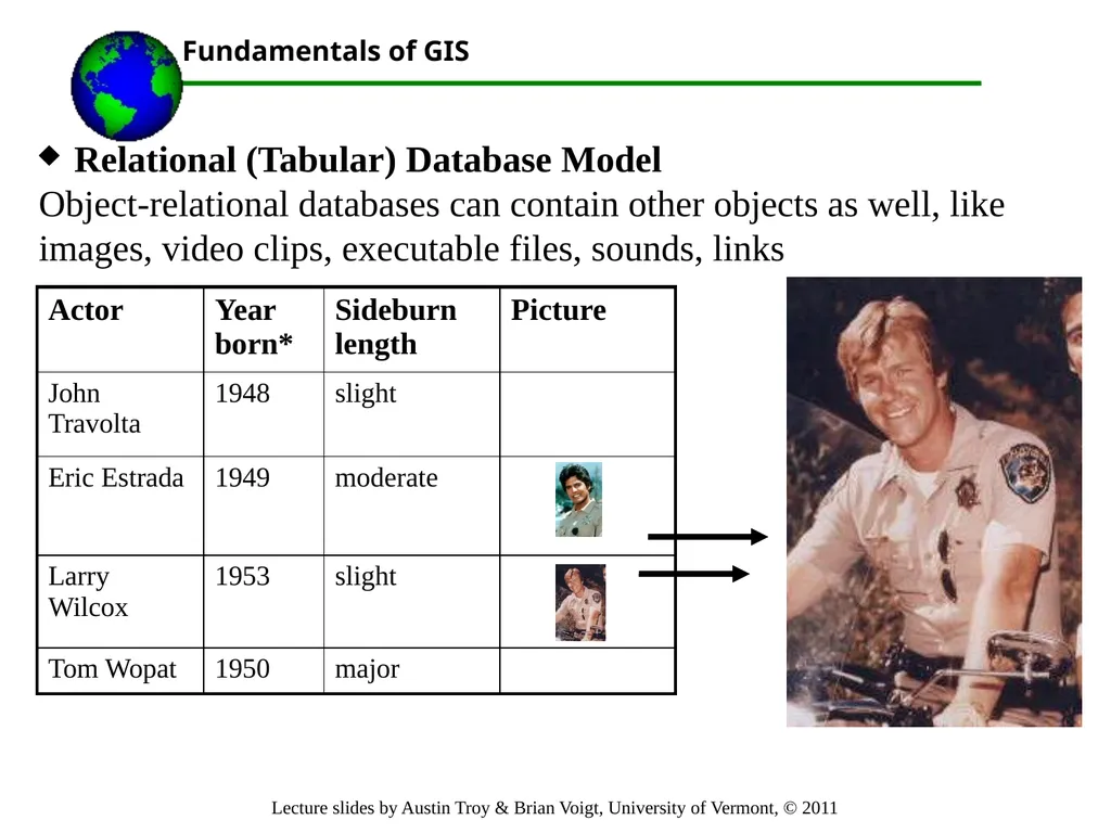
Object-relational databases can contain other objects as well, like images, video clips, executable files, sounds, links<br>
Object-relational databases can contain other objects as well, like images, video clips, executable files, sounds, links<br>
22
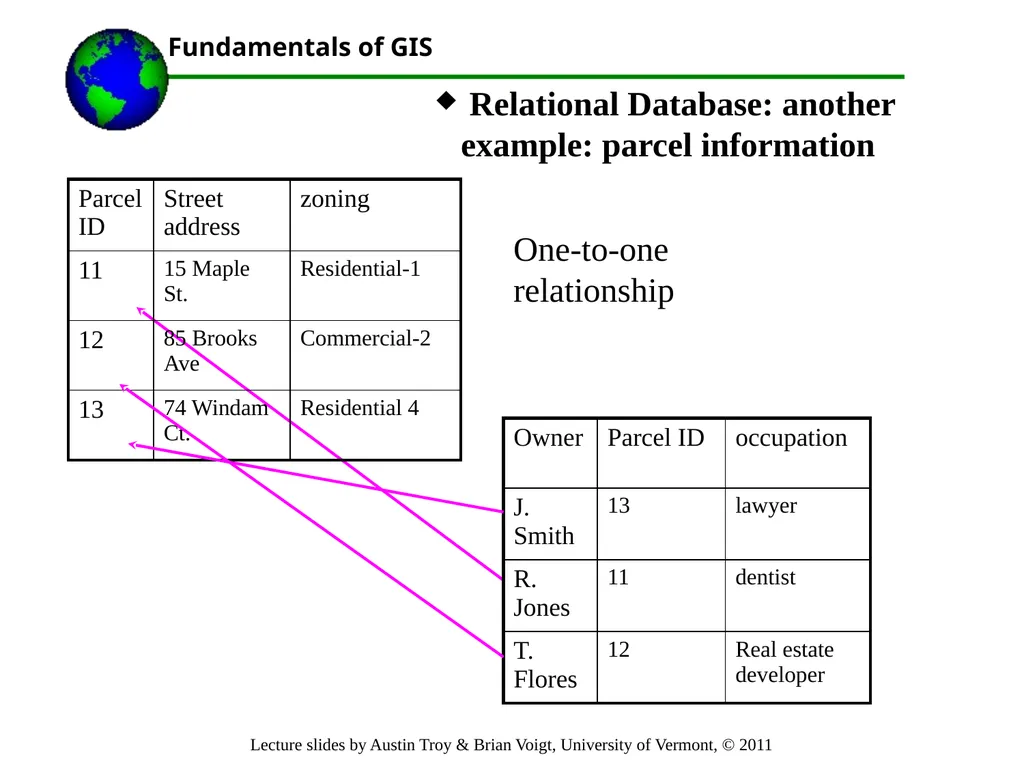
Relational Database: another example: parcel information One-to-one relationship<br>
23
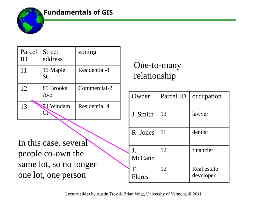
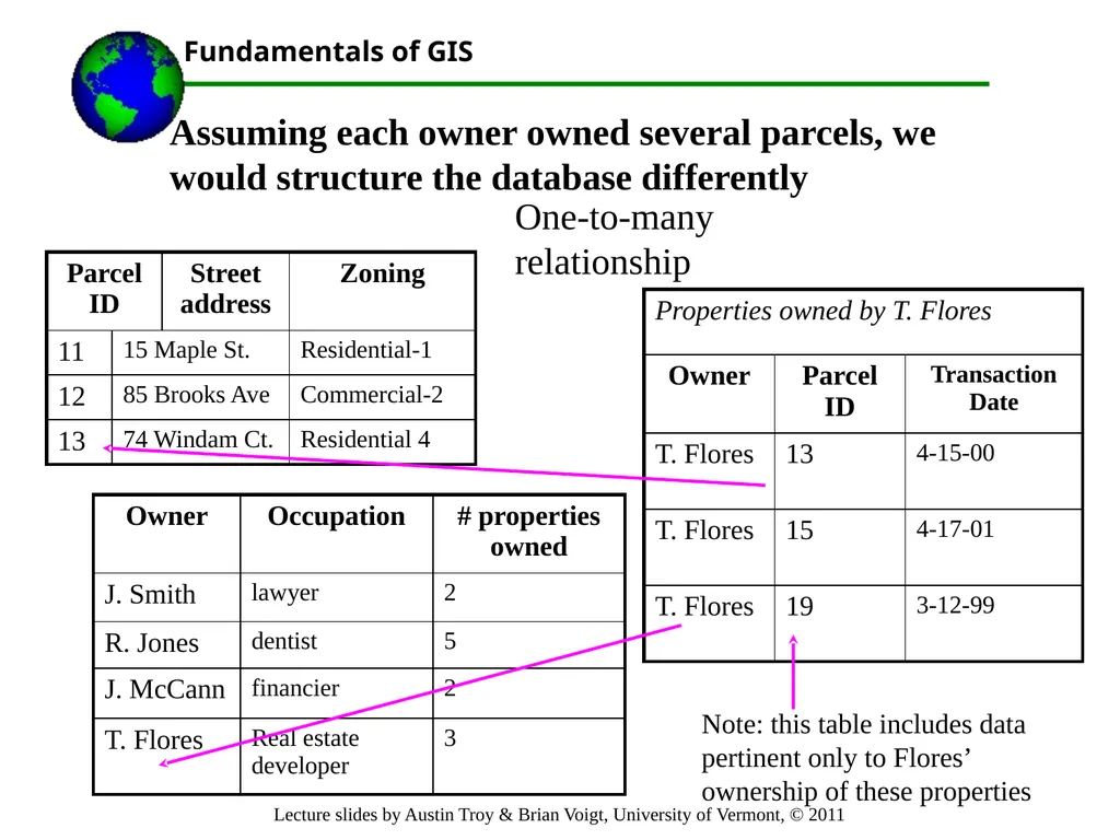
One-to-many relationship In this case, several people co-own the same lot, so no longer one lot, one person<br>
24
Assuming each owner owned several parcels, we would structure the database differently One-to-many relationship Note: this table includes data pertinent only to Flores’ ownership of these properties<br>
25
Example
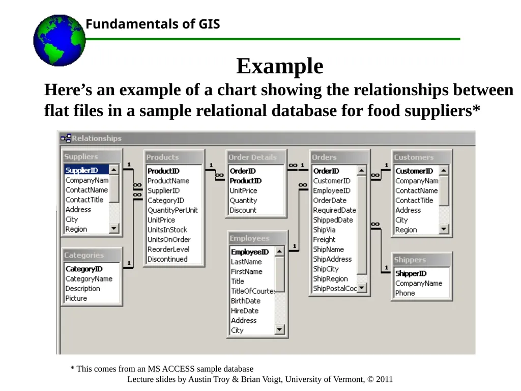
Here’s an example of a chart showing the relationships between flat files in a sample relational database for food suppliers* * This comes from an MS ACCESS sample database<br>
Here’s an example of a chart showing the relationships between flat files in a sample relational database for food suppliers* * This comes from an MS ACCESS sample database<br>
26
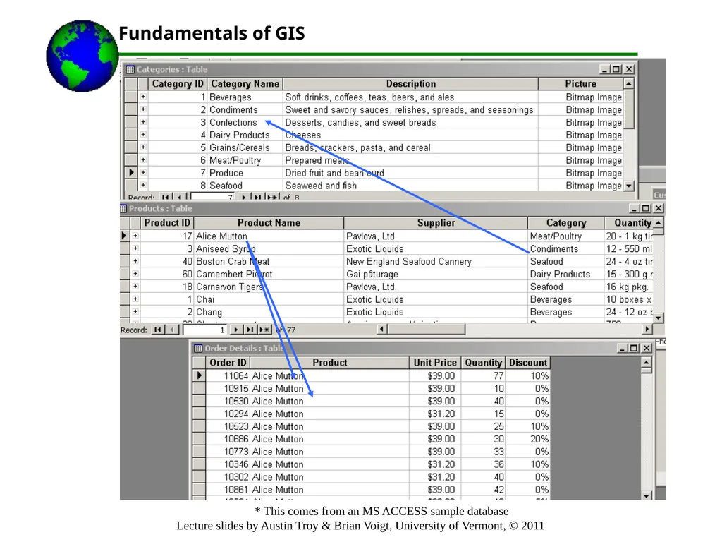
* This comes from an MS ACCESS sample database<br>
27
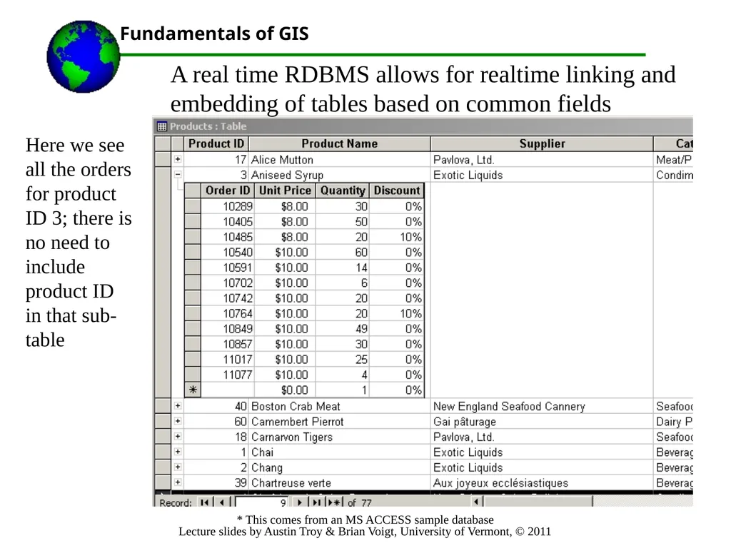
* This comes from an MS ACCESS sample database A real time RDBMS allows for realtime linking and embedding of tables based on common fields Here we see all the orders for product ID 3; there is no need to include product ID in that sub-table<br>
28
Part 2. Queries<br>
29
Queries This is how we ask questions about the data
Queries use mathematical operators, like =, >, <
For multiple criteria queries, we use logical operators, like AND, OR, NOT
Queries can simply select records or perform more advanced operations with those selections, such as make new tables, or summarize values<br>
Queries use mathematical operators, like =, >, <
For multiple criteria queries, we use logical operators, like AND, OR, NOT
Queries can simply select records or perform more advanced operations with those selections, such as make new tables, or summarize values<br>
30
Queries in ArcGIS ArcGIS queries select (highlight) records
When a record is selected, so is its corresponding feature (and vice versa)
To summarize selected values, use the “statistics” function or “summarize” tool
To calculate new values for selected records (based on a query), use the “calculate” tool.<br>
When a record is selected, so is its corresponding feature (and vice versa)
To summarize selected values, use the “statistics” function or “summarize” tool
To calculate new values for selected records (based on a query), use the “calculate” tool.<br>
31
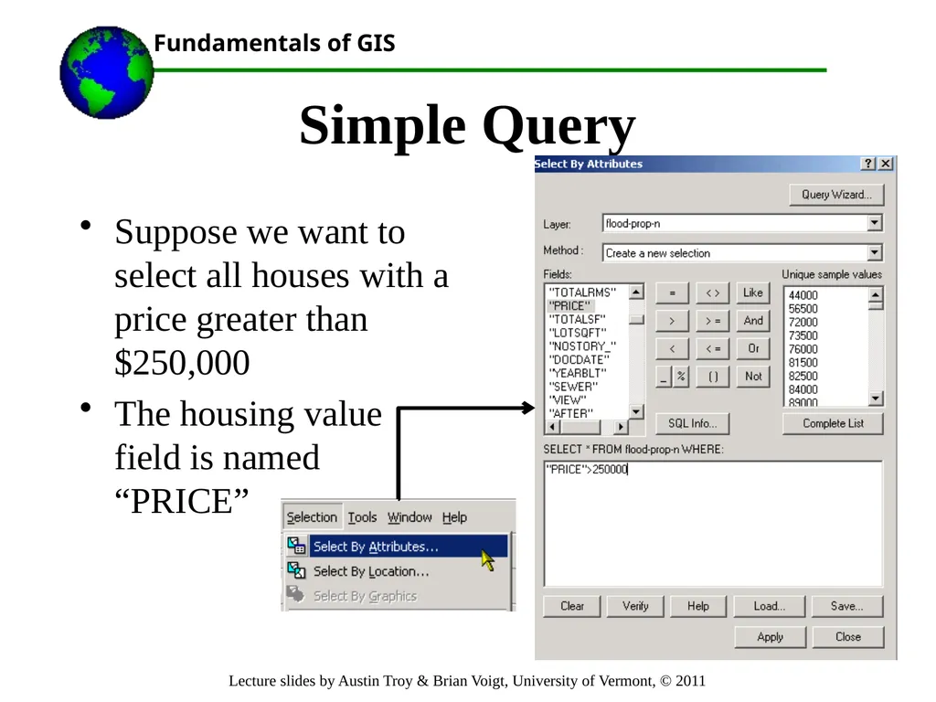
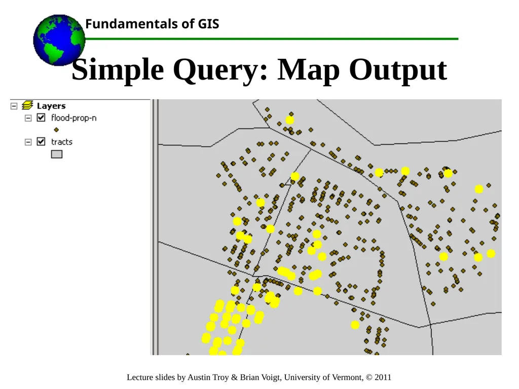
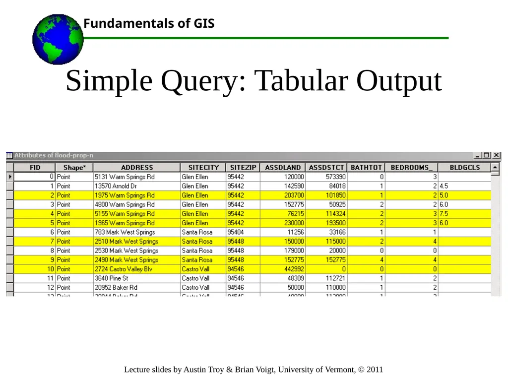
Simple Query Suppose we want to select all houses with a price greater than $250,000
The housing value field is named “PRICE”<br>
The housing value field is named “PRICE”<br>
32
Simple Query: Map Output<br>
33
Simple Query: Tabular Output<br>
34
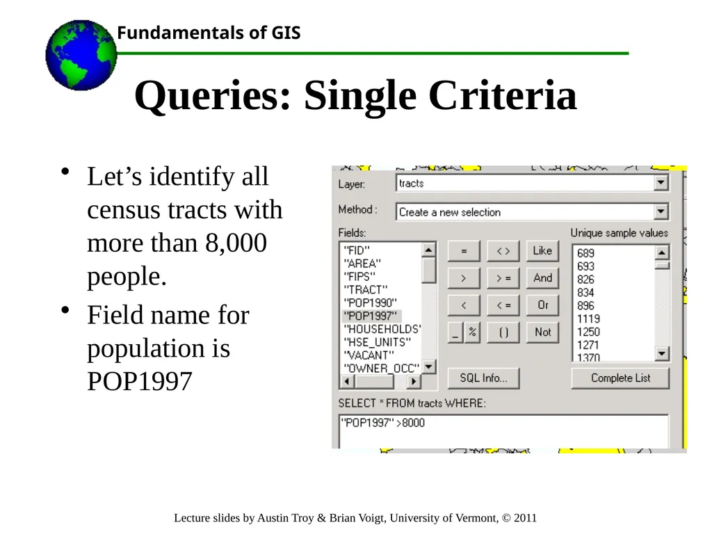
Queries: Single Criteria Let’s identify all census tracts with more than 8,000 people.
Field name for population is POP1997<br>
Field name for population is POP1997<br>
35
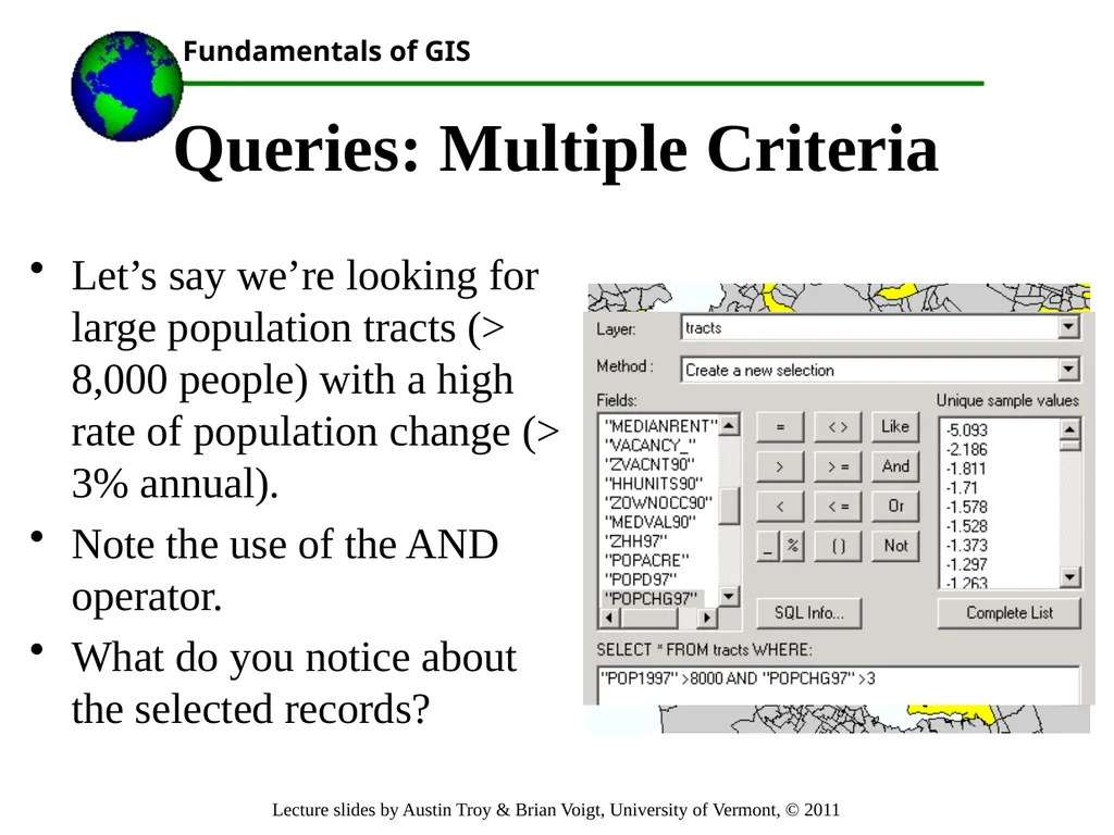
Queries: Multiple Criteria Let’s say we’re looking for large population tracts (> 8,000 people) with a high rate of population change (> 3% annual).
Note the use of the AND operator.
What do you notice about the selected records?<br>
Note the use of the AND operator.
What do you notice about the selected records?<br>
36
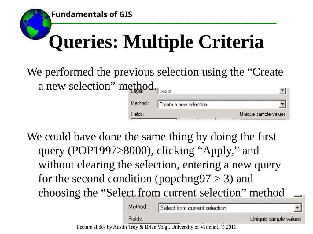
Queries: Multiple Criteria We performed the previous selection using the “Create a new selection” method.
We could have done the same thing by doing the first query (POP1997>8000), clicking “Apply,” and without clearing the selection, entering a new query for the second condition (popchng97 > 3) and choosing the “Select from current selection” method<br>
We could have done the same thing by doing the first query (POP1997>8000), clicking “Apply,” and without clearing the selection, entering a new query for the second condition (popchng97 > 3) and choosing the “Select from current selection” method<br>
37
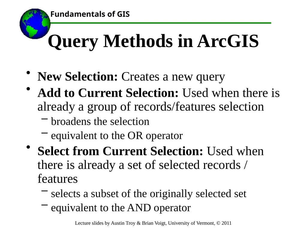
Query Methods in ArcGIS New Selection: Creates a new query
Add to Current Selection: Used when there is already a group of records/features selection
broadens the selection
equivalent to the OR operator
Select from Current Selection: Used when there is already a set of selected records / features
selects a subset of the originally selected set
equivalent to the AND operator<br>
Add to Current Selection: Used when there is already a group of records/features selection
broadens the selection
equivalent to the OR operator
Select from Current Selection: Used when there is already a set of selected records / features
selects a subset of the originally selected set
equivalent to the AND operator<br>
38
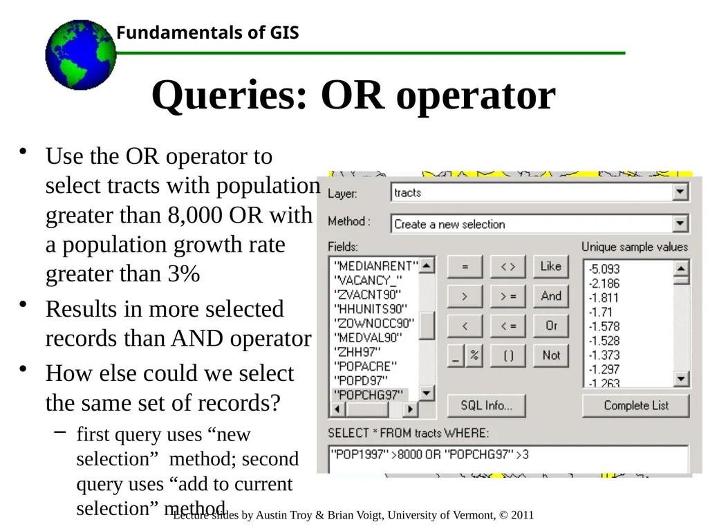
Queries: OR operator Use the OR operator to select tracts with population greater than 8,000 OR with a population growth rate greater than 3%
Results in more selected records than AND operator
How else could we select the same set of records?
first query uses “new selection” method; second query uses “add to current selection” method<br>
Results in more selected records than AND operator
How else could we select the same set of records?
first query uses “new selection” method; second query uses “add to current selection” method<br>
39
Queries: Strings
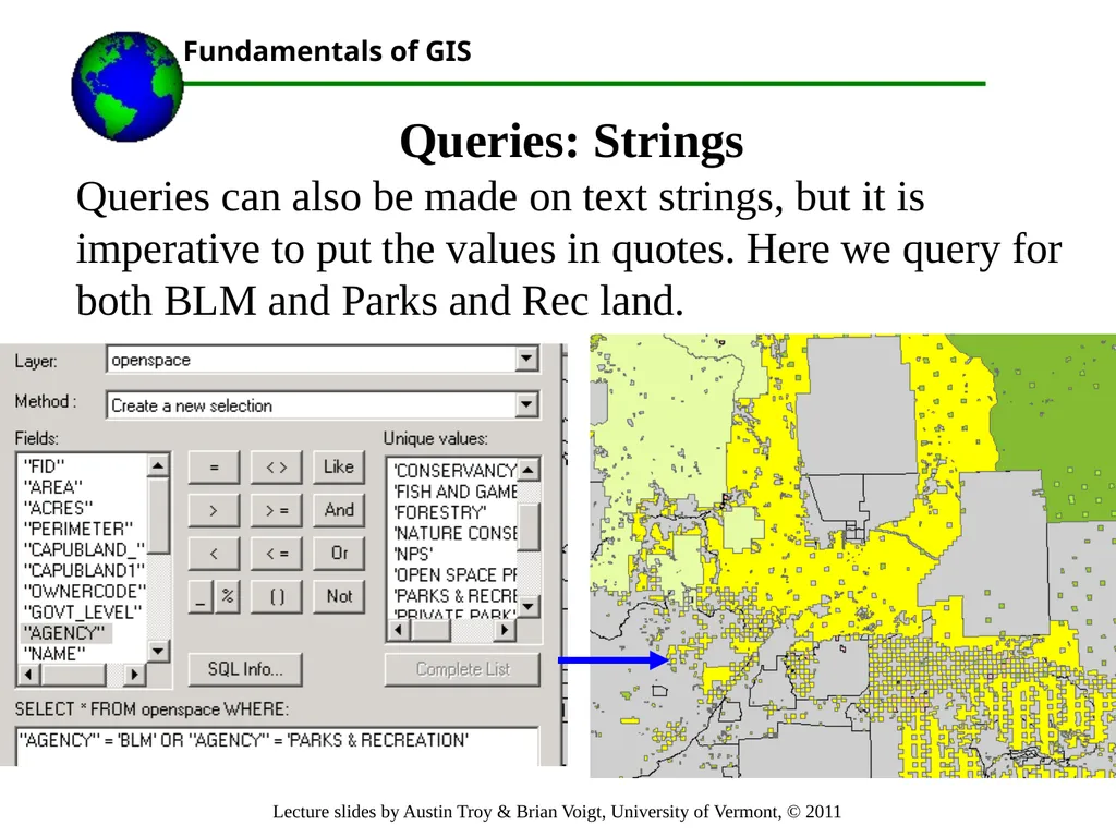
Queries can also be made on text strings, but it is imperative to put the values in quotes. Here we query for both BLM and Parks and Rec land.<br>
Queries can also be made on text strings, but it is imperative to put the values in quotes. Here we query for both BLM and Parks and Rec land.<br>
40
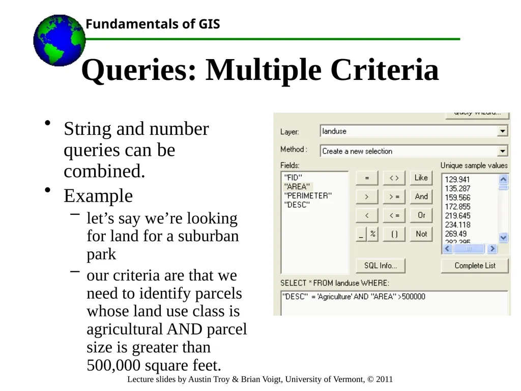
Queries: Multiple Criteria String and number queries can be combined.
Example
let’s say we’re looking for land for a suburban park
our criteria are that we need to identify parcels whose land use class is agricultural AND parcel size is greater than 500,000 square feet.<br>
Example
let’s say we’re looking for land for a suburban park
our criteria are that we need to identify parcels whose land use class is agricultural AND parcel size is greater than 500,000 square feet.<br>
41
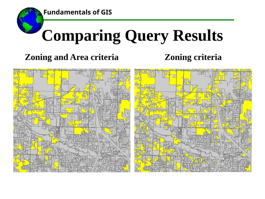
Comparing Query Results Zoning and Area criteria Zoning criteria<br>
42
View the selection
Re-query the selection
Compute statistics on the selection
Calculate the value of a new field or update the value of an existing field based on the value of one (or more) attributes or a user-specified formula
Create a new shapefile / feature class from the selection ArcGIS Query Results<br>
Re-query the selection
Compute statistics on the selection
Calculate the value of a new field or update the value of an existing field based on the value of one (or more) attributes or a user-specified formula
Create a new shapefile / feature class from the selection ArcGIS Query Results<br>
43
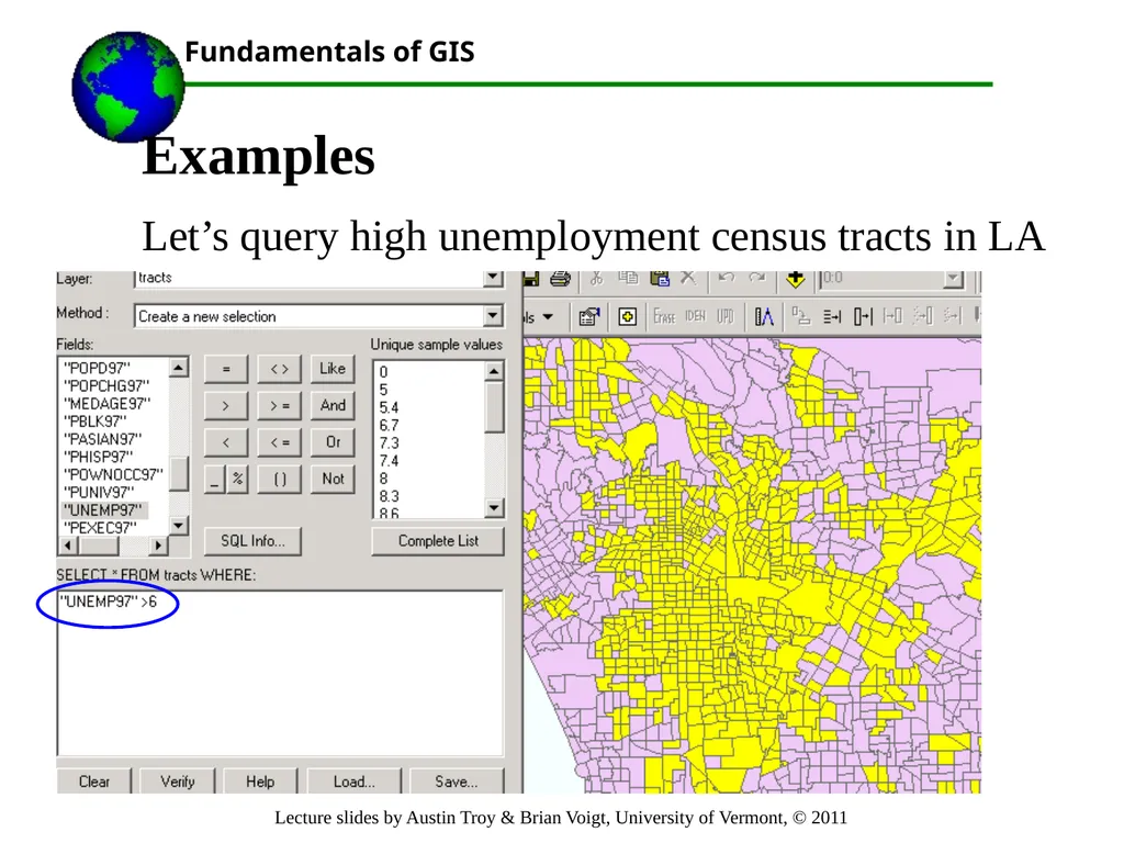
Examples
Let’s query high unemployment census tracts in LA<br>
Let’s query high unemployment census tracts in LA<br>
44
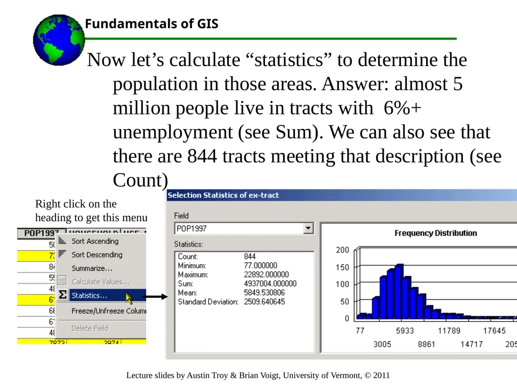
Now let’s calculate “statistics” to determine the population in those areas. Answer: almost 5 million people live in tracts with 6%+ unemployment (see Sum). We can also see that there are 844 tracts meeting that description (see Count) Right click on the heading to get this menu<br>
45
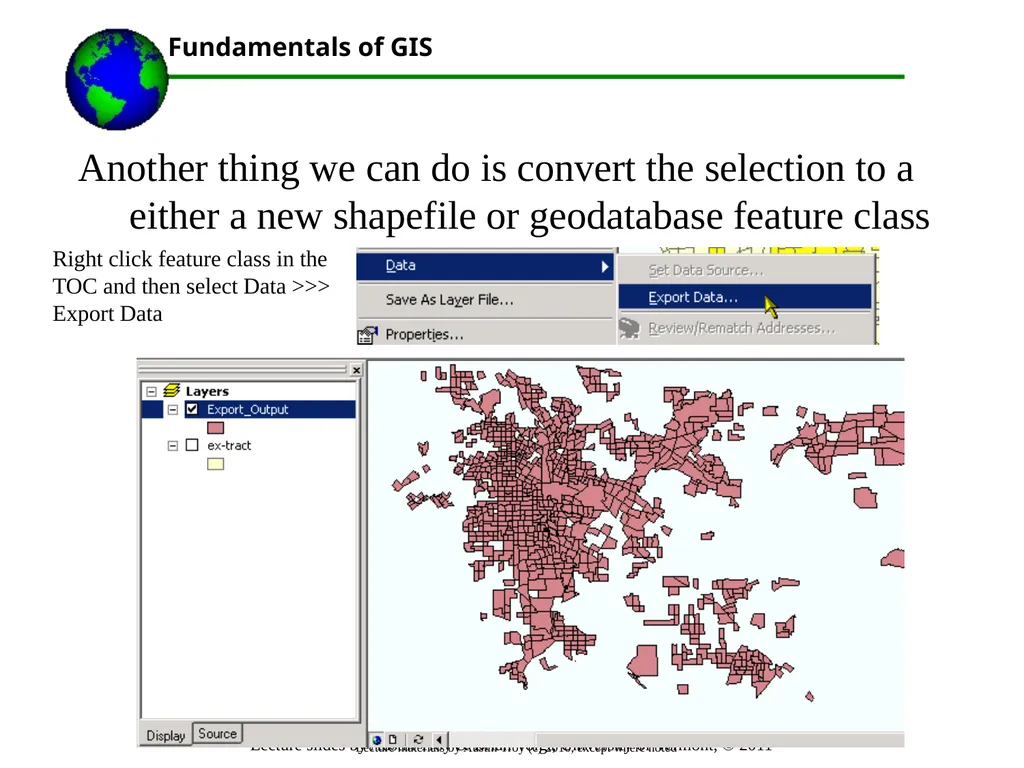
Lecture materials by Austin Troy (c) 2010, except where noted Another thing we can do is convert the selection to a either a new shapefile or geodatabase feature class Right click feature class in the TOC and then select Data >>> Export Data<br>
46
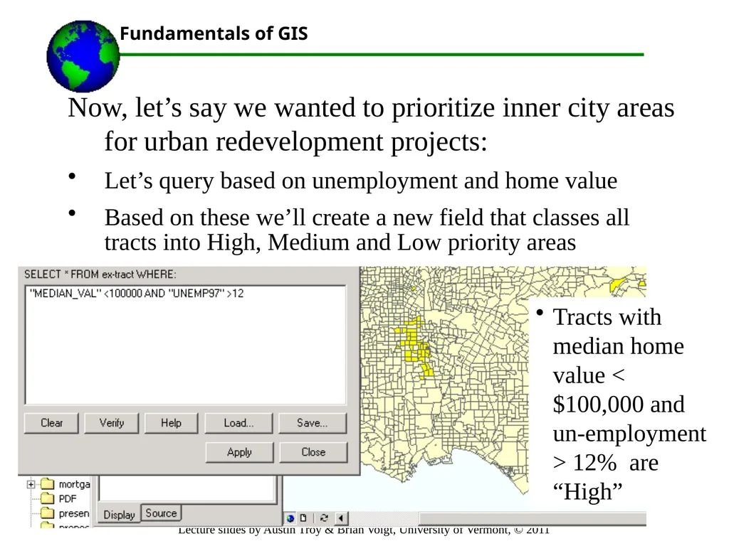
Now, let’s say we wanted to prioritize inner city areas for urban redevelopment projects:
Let’s query based on unemployment and home value
Based on these we’ll create a new field that classes all tracts into High, Medium and Low priority areas Tracts with median home value < $100,000 and un-employment > 12% are “High”<br>
Let’s query based on unemployment and home value
Based on these we’ll create a new field that classes all tracts into High, Medium and Low priority areas Tracts with median home value < $100,000 and un-employment > 12% are “High”<br>
47
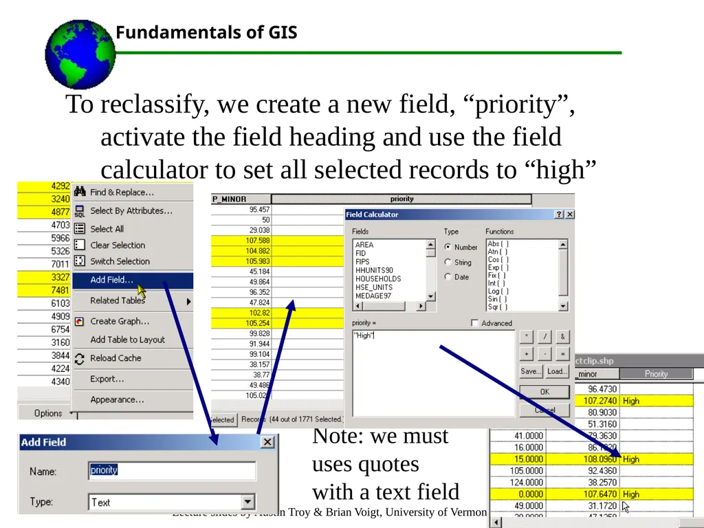
To reclassify, we create a new field, “priority”, activate the field heading and use the field calculator to set all selected records to “high” Note: we must uses quotes with a text field<br>
48
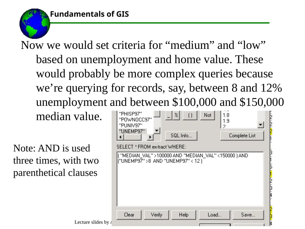
Now we would set criteria for “medium” and “low” based on unemployment and home value. These would probably be more complex queries because we’re querying for records, say, between 8 and 12% unemployment and between $100,000 and $150,000 median value. Note: AND is used three times, with two parenthetical clauses<br>
49
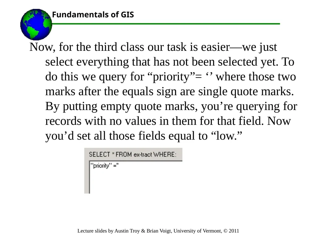
Now, for the third class our task is easier—we just select everything that has not been selected yet. To do this we query for “priority”= ‘’ where those two marks after the equals sign are single quote marks. By putting empty quote marks, you’re querying for records with no values in them for that field. Now you’d set all those fields equal to “low.”<br>
50
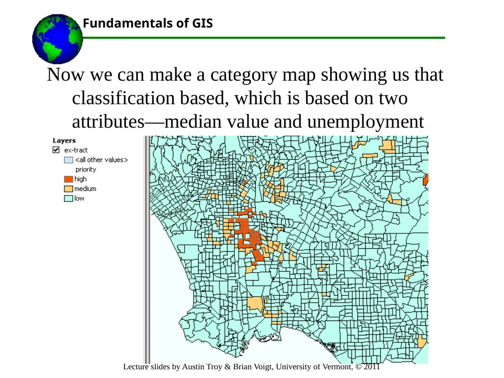
Now we can make a category map showing us that classification based, which is based on two attributes—median value and unemployment<br>
51
Another example:
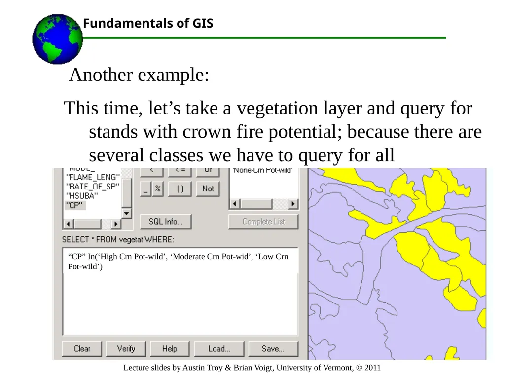
This time, let’s take a vegetation layer and query for stands with crown fire potential; because there are several classes we have to query for all “CP” In(‘High Crn Pot-wild’, ‘Moderate Crn Pot-wid’, ‘Low Crn Pot-wild’)<br>
This time, let’s take a vegetation layer and query for stands with crown fire potential; because there are several classes we have to query for all “CP” In(‘High Crn Pot-wild’, ‘Moderate Crn Pot-wid’, ‘Low Crn Pot-wild’)<br>
52
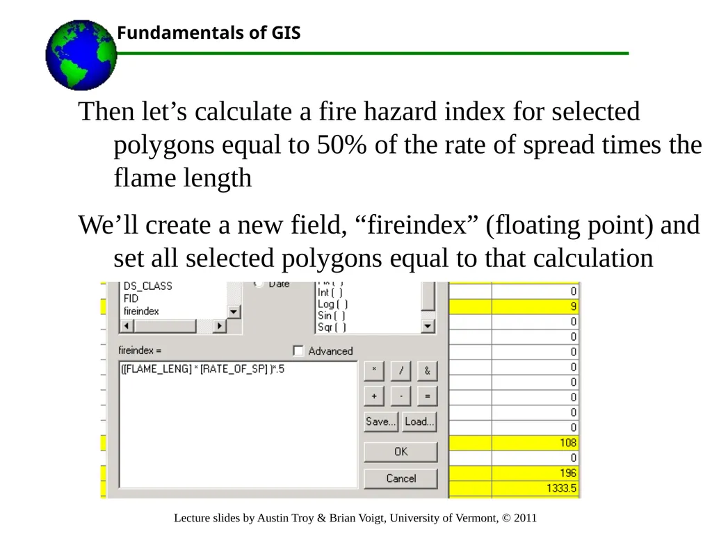
Then let’s calculate a fire hazard index for selected polygons equal to 50% of the rate of spread times the flame length
We’ll create a new field, “fireindex” (floating point) and set all selected polygons equal to that calculation<br>
We’ll create a new field, “fireindex” (floating point) and set all selected polygons equal to that calculation<br>
53
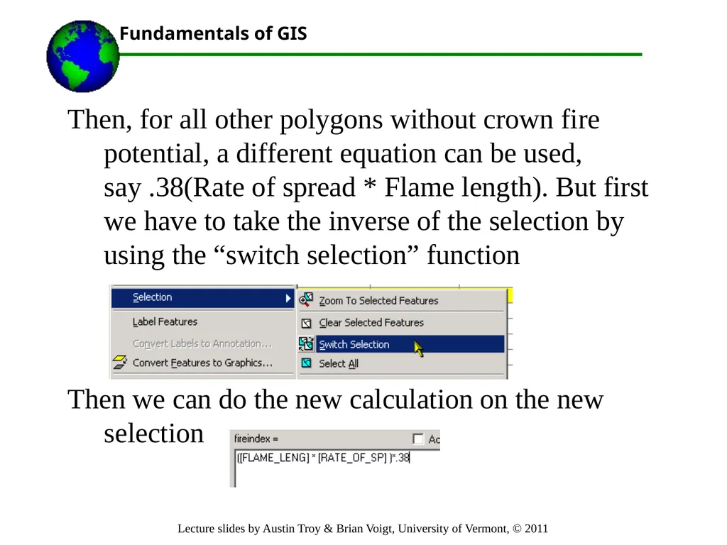
Then, for all other polygons without crown fire potential, a different equation can be used, say .38(Rate of spread * Flame length). But first we have to take the inverse of the selection by using the “switch selection” function
Then we can do the new calculation on the new selection<br>
Then we can do the new calculation on the new selection<br>
54
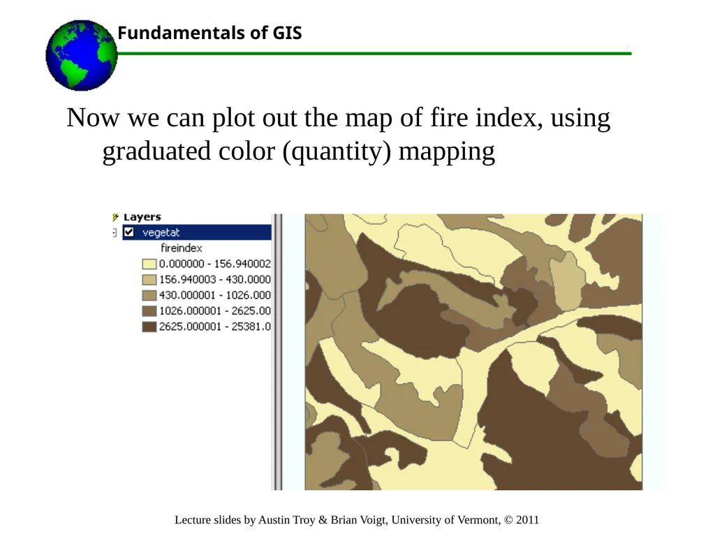
Now we can plot out the map of fire index, using graduated color (quantity) mapping<br>
55
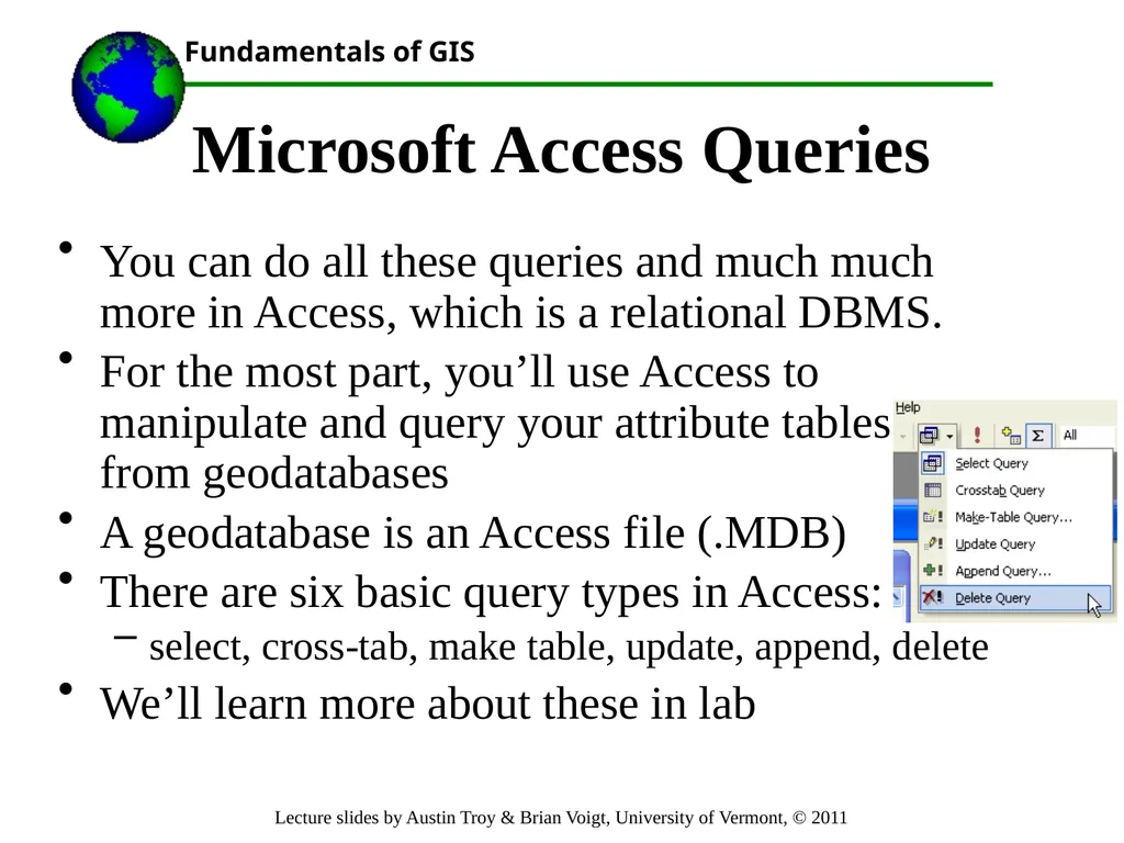
Microsoft Access Queries You can do all these queries and much much more in Access, which is a relational DBMS.
For the most part, you’ll use Access to manipulate and query your attribute tables from geodatabases
A geodatabase is an Access file (.MDB)
There are six basic query types in Access:
select, cross-tab, make table, update, append, delete
We’ll learn more about these in lab<br>
For the most part, you’ll use Access to manipulate and query your attribute tables from geodatabases
A geodatabase is an Access file (.MDB)
There are six basic query types in Access:
select, cross-tab, make table, update, append, delete
We’ll learn more about these in lab<br>
56
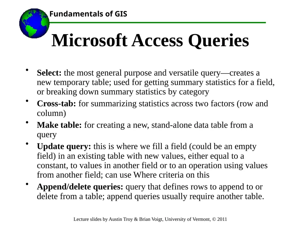
Microsoft Access Queries Select: the most general purpose and versatile query—creates a new temporary table; used for getting summary statistics for a field, or breaking down summary statistics by category
Cross-tab: for summarizing statistics across two factors (row and column)
Make table: for creating a new, stand-alone data table from a query
Update query: this is where we fill a field (could be an empty field) in an existing table with new values, either equal to a constant, to values in another field or to an operation using values from another field; can use Where criteria on this
Append/delete queries: query that defines rows to append to or delete from a table; append queries usually require another table.<br>
Cross-tab: for summarizing statistics across two factors (row and column)
Make table: for creating a new, stand-alone data table from a query
Update query: this is where we fill a field (could be an empty field) in an existing table with new values, either equal to a constant, to values in another field or to an operation using values from another field; can use Where criteria on this
Append/delete queries: query that defines rows to append to or delete from a table; append queries usually require another table.<br>
57
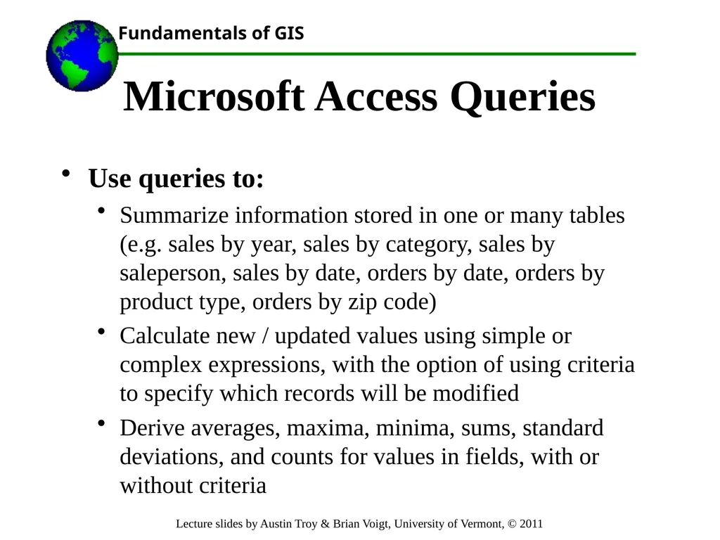
Microsoft Access Queries Use queries to:
Summarize information stored in one or many tables (e.g. sales by year, sales by category, sales by saleperson, sales by date, orders by date, orders by product type, orders by zip code)
Calculate new / updated values using simple or complex expressions, with the option of using criteria to specify which records will be modified
Derive averages, maxima, minima, sums, standard deviations, and counts for values in fields, with or without criteria<br>
Summarize information stored in one or many tables (e.g. sales by year, sales by category, sales by saleperson, sales by date, orders by date, orders by product type, orders by zip code)
Calculate new / updated values using simple or complex expressions, with the option of using criteria to specify which records will be modified
Derive averages, maxima, minima, sums, standard deviations, and counts for values in fields, with or without criteria<br>
58
Microsoft Access Queries
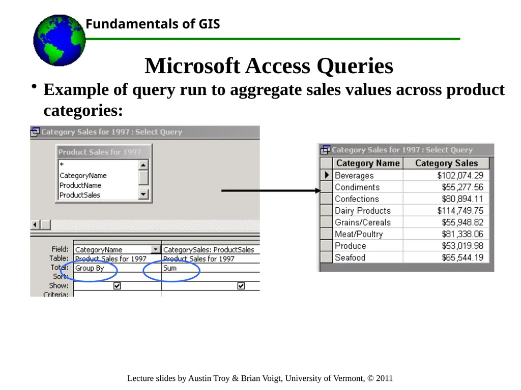
Example of query run to aggregate sales values across product categories:<br>
Example of query run to aggregate sales values across product categories:<br>
59
Relational attribute queries
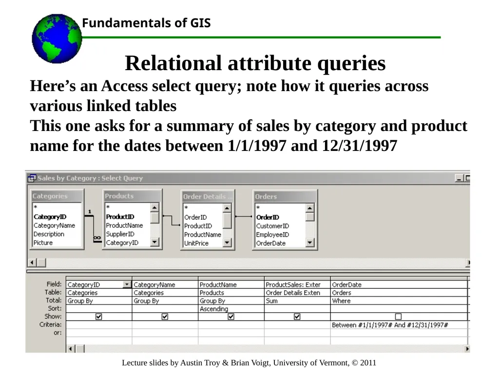
Here’s an Access select query; note how it queries across various linked tables
This one asks for a summary of sales by category and product name for the dates between 1/1/1997 and 12/31/1997<br>
Here’s an Access select query; note how it queries across various linked tables
This one asks for a summary of sales by category and product name for the dates between 1/1/1997 and 12/31/1997<br>
60
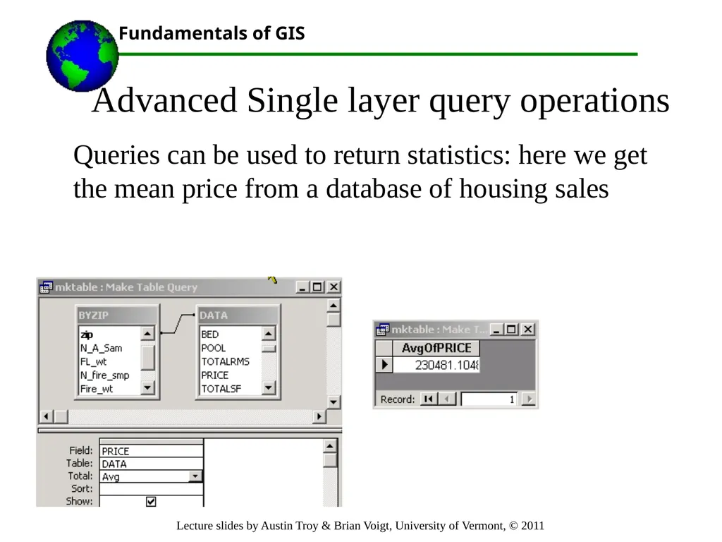
Advanced Single layer query operations Queries can be used to return statistics: here we get the mean price from a database of housing sales<br>
61
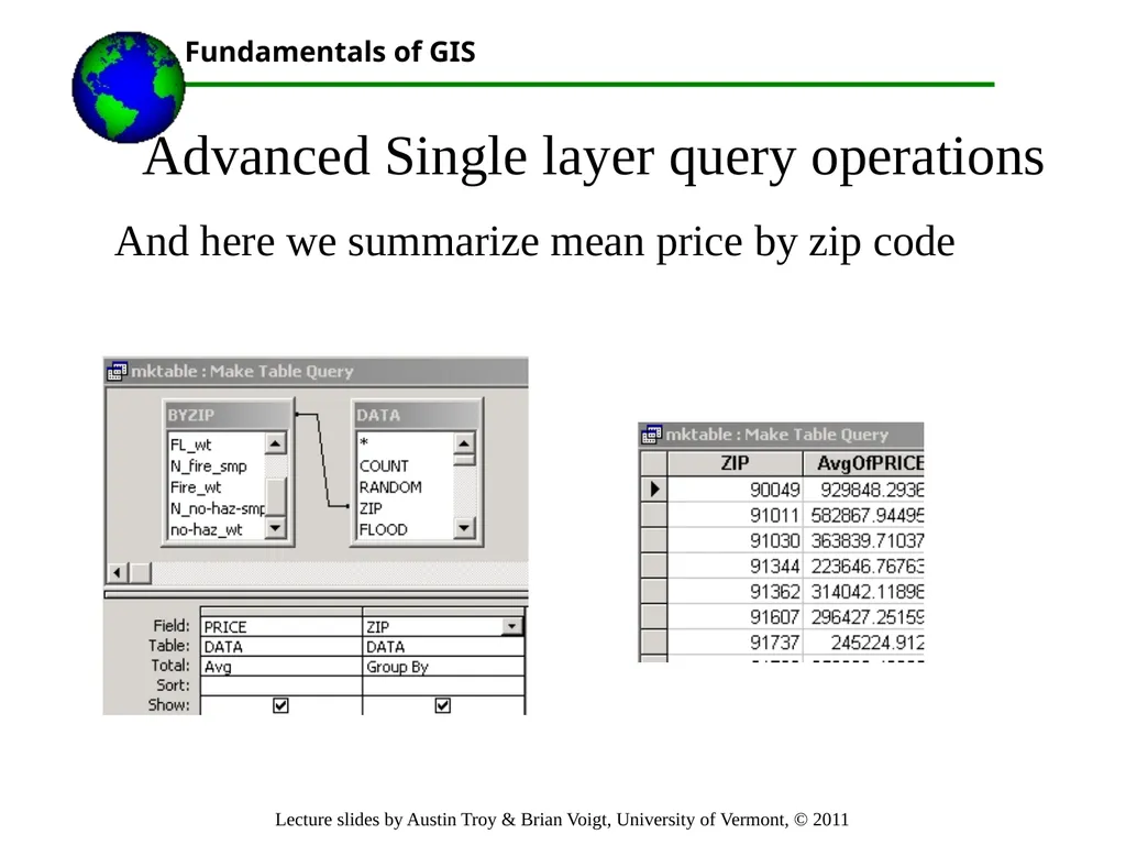
Advanced Single layer query operations And here we summarize mean price by zip code<br>
62
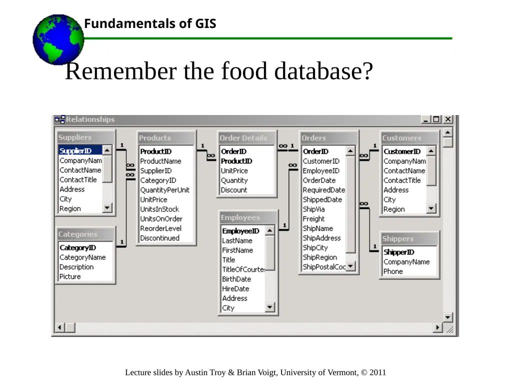
Remember the food database?<br>
63
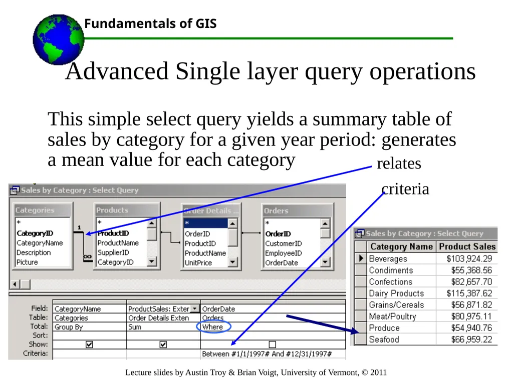
Advanced Single layer query operations This simple select query yields a summary table of sales by category for a given year period: generates a mean value for each category criteria relates<br>
64
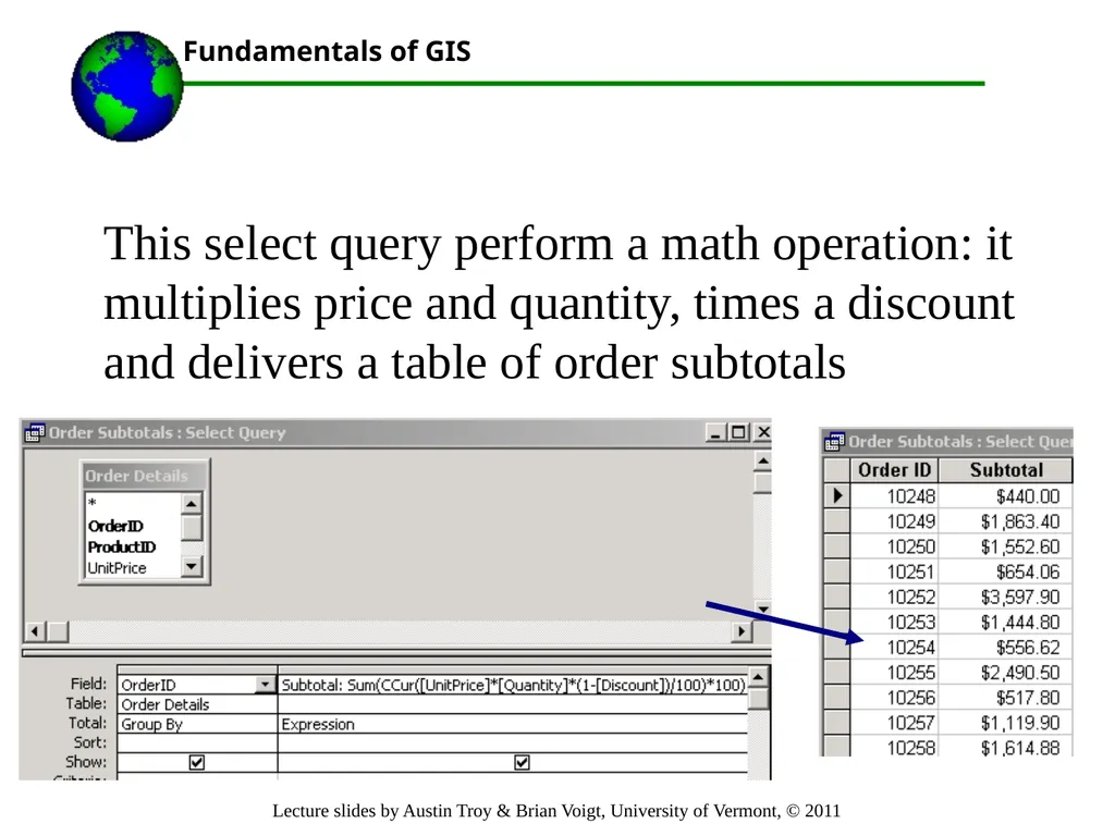
This select query perform a math operation: it multiplies price and quantity, times a discount and delivers a table of order subtotals<br>
65
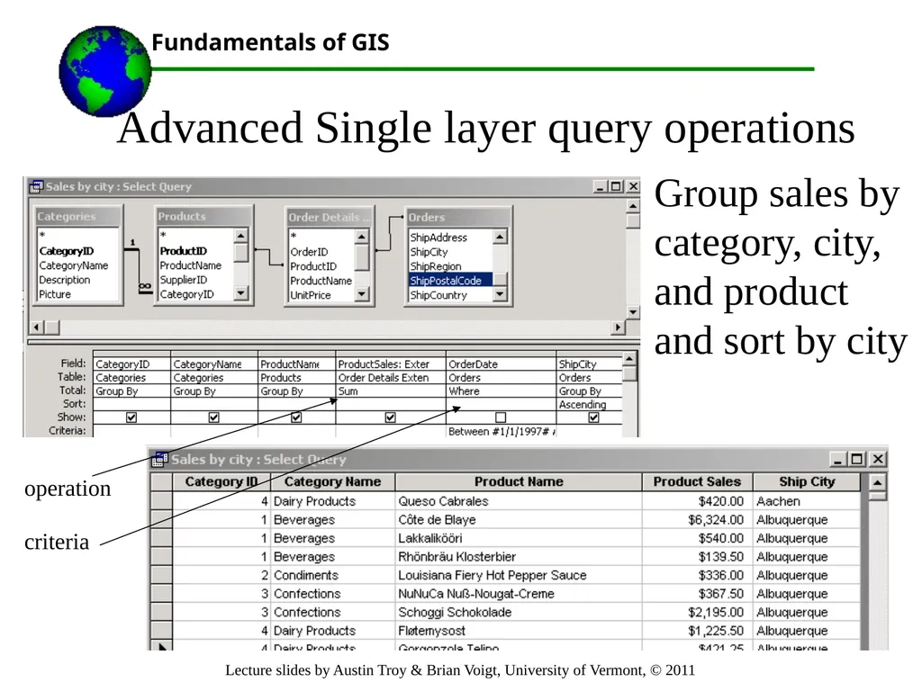
Advanced Single layer query operations Group sales by category, city, and product and sort by city operation criteria<br>
66
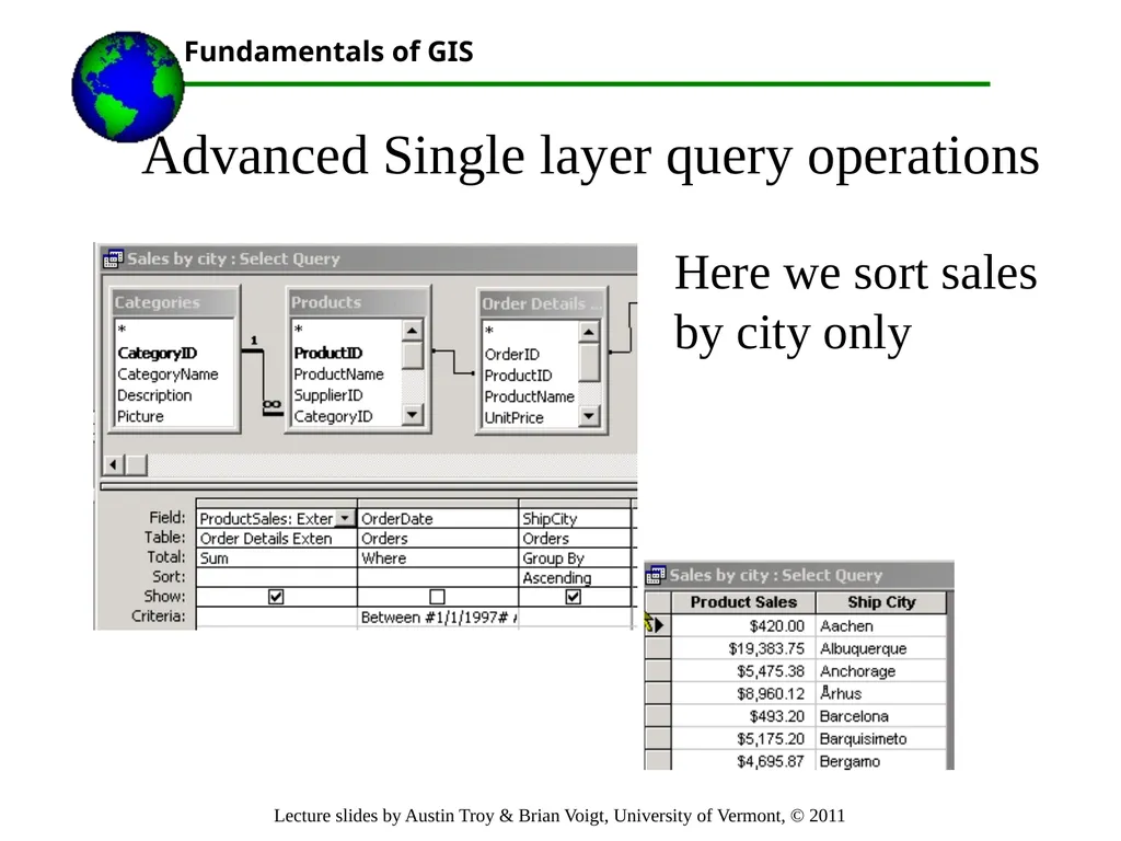
Advanced Single layer query operations Here we sort sales by city only<br>
67
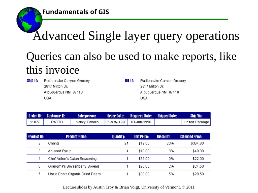
Advanced Single layer query operations Queries can also be used to make reports, like this invoice<br>
68
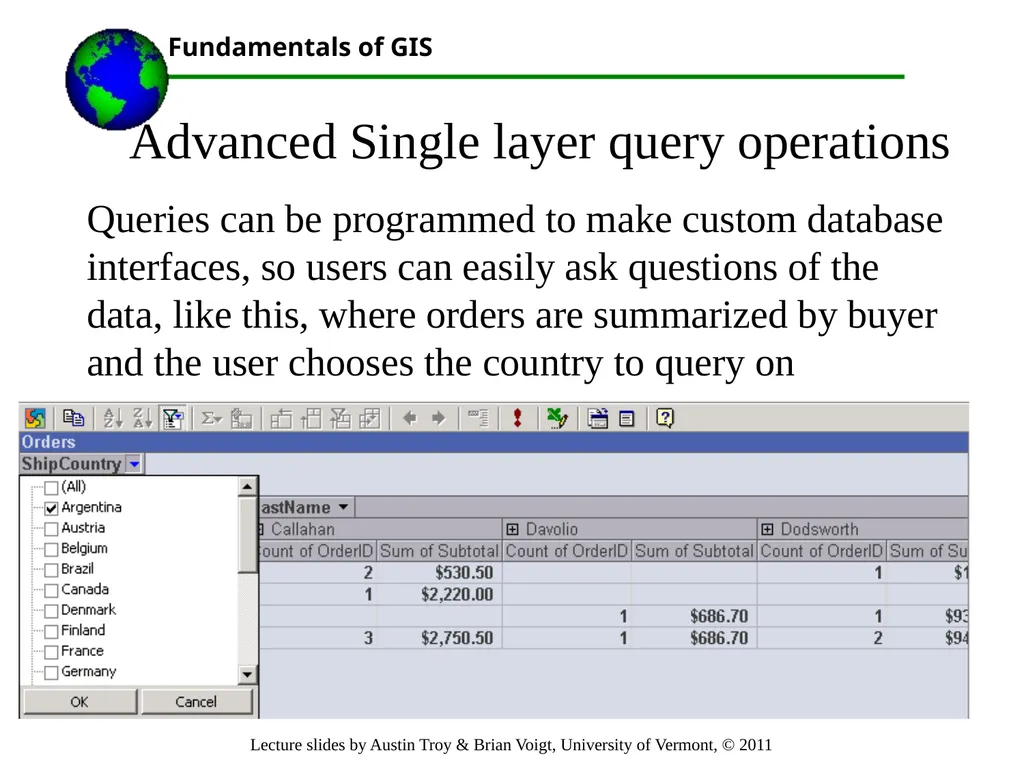
Advanced Single layer query operations Queries can be programmed to make custom database interfaces, so users can easily ask questions of the data, like this, where orders are summarized by buyer and the user chooses the country to query on<br>