
Lecture 8- Performance Evaluation Dr. Sampath
Description: Lecture 8- Performance Evaluation Dr. Sampath Jayarathna Cal Poly Pomona Credit for some of the slides in this lecture goes to Prof. Ray Mooney at UT Austin Prof. Rong Jin at MSU CS 620 DASC 600 Introduction to Data Science Analytics
Related Topics
Download Presentation
"Lecture 8- Performance Evaluation Dr. Sampath" is the property of its rightful owner. Permission is granted to download and print the materials on this website for personal, non-commercial use only, and to display it on your personal computer provided you do not modify the materials and that you retain all copyright notices contained in the materials. By downloading content from our website, you accept the terms of this agreement.
Presentation Transcript
slide1. Lecture 8- Performance Evaluation Dr. Sampath Jayarathna
Cal Poly Pomona Credit for some of the slides in this lecture goes to Prof. Ray Mooney at UT Austin & Prof. Rong Jin at MSU CS 620 / DASC 600
Introduction to Data Science & Analytics<br>
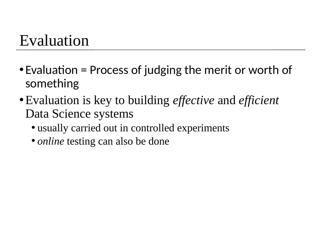
slide2. Evaluation Evaluation = Process of judging the merit or worth of something
Evaluation is key to building effective and efficient Data Science systems
usually carried out in controlled experiments
online testing can also be done<br>
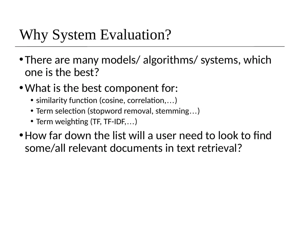
slide3. Why System Evaluation? There are many models/ algorithms/ systems, which one is the best?
What is the best component for:
similarity function (cosine, correlation,…)
Term selection (stopword removal, stemming…)
Term weighting (TF, TF-IDF,…)
How far down the list will a user need to look to find some/all relevant documents in text retrieval?<br>
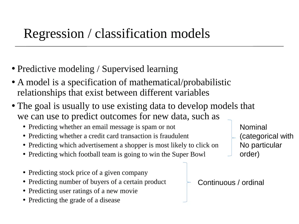
slide4. Regression / classification models Predictive modeling / Supervised learning
A model is a specification of mathematical/probabilistic relationships that exist between different variables
The goal is usually to use existing data to develop models that we can use to predict outcomes for new data, such as
Predicting whether an email message is spam or not
Predicting whether a credit card transaction is fraudulent
Predicting which advertisement a shopper is most likely to click on
Predicting which football team is going to win the Super Bowl
Predicting stock price of a given company
Predicting number of buyers of a certain product
Predicting user ratings of a new movie
Predicting the grade of a disease Nominal
(categorical with
No particular order) Continuous / ordinal<br>
slide5. Performance evaluation How predictive is the model we learned?
For regression, usually R2 or MSE
For classification, many options (discuss later today)
Accuracy can be used, with caution
Performance on the training data (data used to build models) is not a good indicator of performance on future data
Q: Why?
A: Because new data will probably not be exactly the same as the training data!<br>
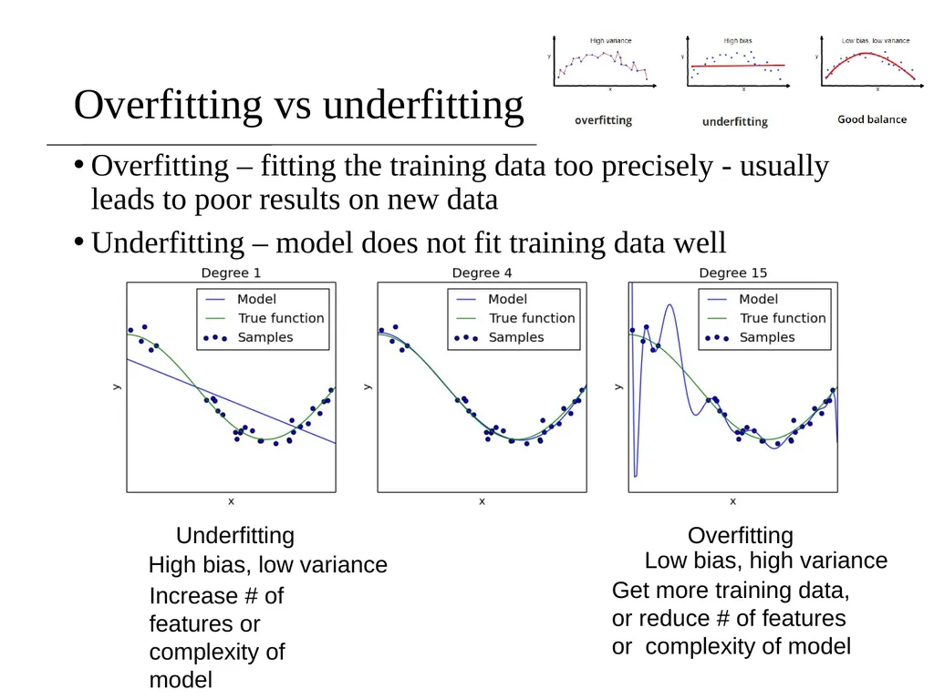
slide6. Overfitting vs underfitting Underfitting Overfitting High bias, low variance Low bias, high variance Increase # of features or complexity of model Get more training data, or reduce # of features or complexity of model Overfitting – fitting the training data too precisely - usually leads to poor results on new data
Underfitting – model does not fit training data well<br>
slide7. Evaluation on “LARGE” data If many (thousands) of examples are available, then how can we evaluate our model?
A simple evaluation is sufficient
Randomly split data into training and test sets (e.g. 2/3 for train, 1/3 for test)
For classification, make sure training and testing have similar distribution of class labels
Build a model using the train set and evaluate it using the test set.<br>
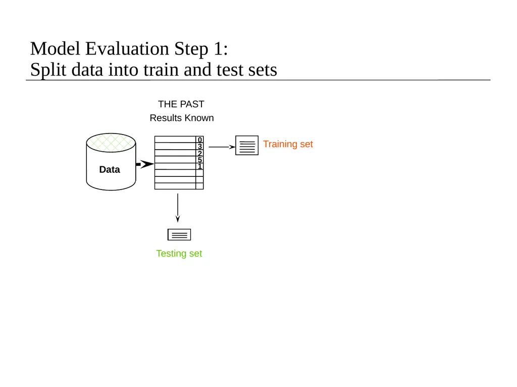
slide8. Model Evaluation Step 1: Split data into train and test sets Results Known 0 3 2 5 1 THE PAST Training set Testing set<br>
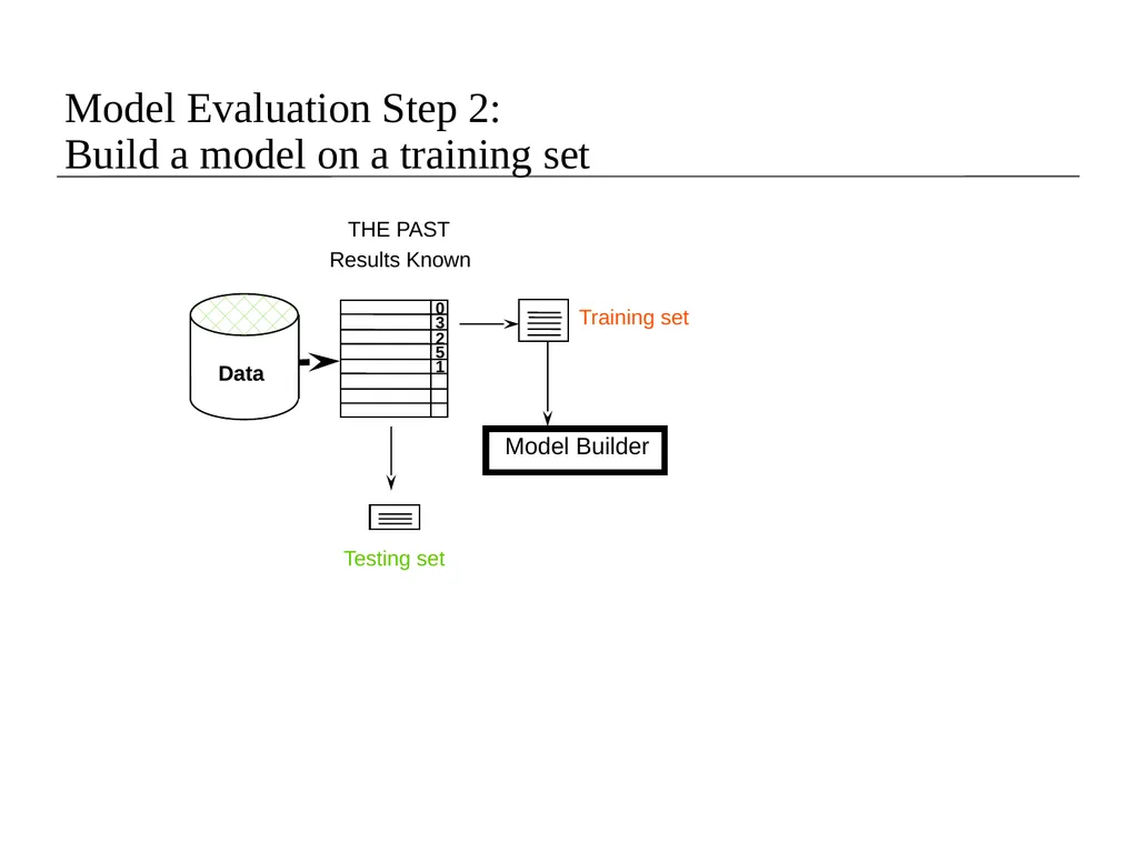
slide9. Model Evaluation Step 2: Build a model on a training set Results Known THE PAST Model Builder Testing set 0 3 2 5 1<br>
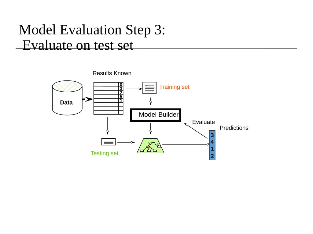
slide10. Model Evaluation Step 3: Evaluate on test set Predictions Results Known Training set Testing set Model Builder Evaluate 3
4
1
2 0 3 2 5 1<br>
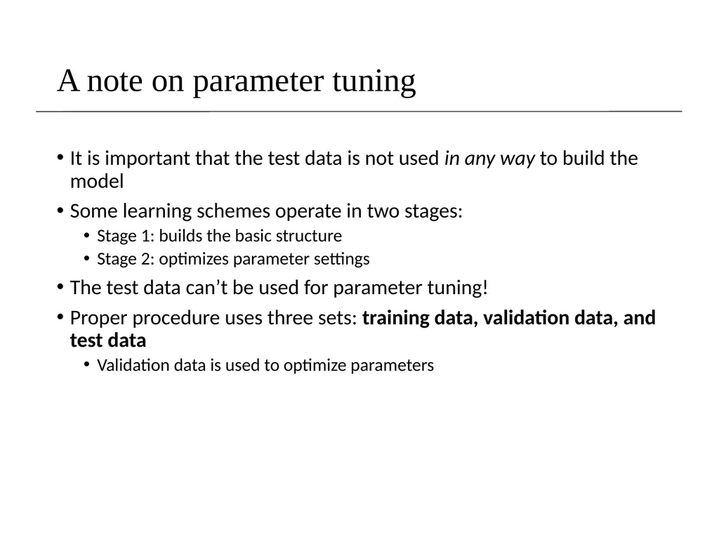
slide11. A note on parameter tuning It is important that the test data is not used in any way to build the model
Some learning schemes operate in two stages:
Stage 1: builds the basic structure
Stage 2: optimizes parameter settings
The test data can’t be used for parameter tuning!
Proper procedure uses three sets: training data, validation data, and test data
Validation data is used to optimize parameters<br>
slide12. Evaluation on “small” data, 1 The holdout method reserves a certain amount for testing and uses the remainder for training
Usually: one third for testing, the rest for training
For “unbalanced” datasets, samples might not be representative
Few or none instances of some classes
Stratified sample: advanced version of balancing the data
Make sure that each class is represented with approximately equal proportions in both subsets<br>
slide13. Evaluation on “small” data, 2 What if we have a small data set?
The chosen 2/3 for training may not be representative.
The chosen 1/3 for testing may not be representative.<br>
slide14. Cross-validation Cross-validation more useful in small datasets
First step: data is split into k subsets of equal size
Second step: each subset in turn is used for testing and the remainder for training
This is called k-fold cross-validation
For classification, often the subsets are stratified before the cross-validation is performed
The error estimates are averaged to yield an overall error estimate<br>
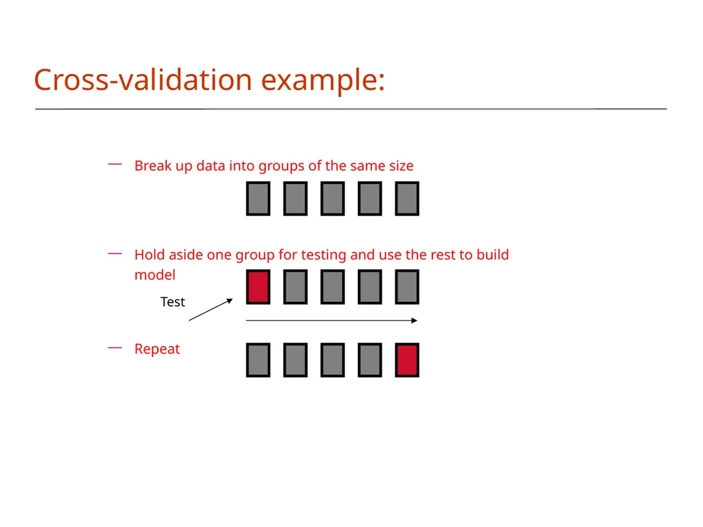
slide15. 15 Cross-validation example: Break up data into groups of the same size
Hold aside one group for testing and use the rest to build model
Repeat Test<br>
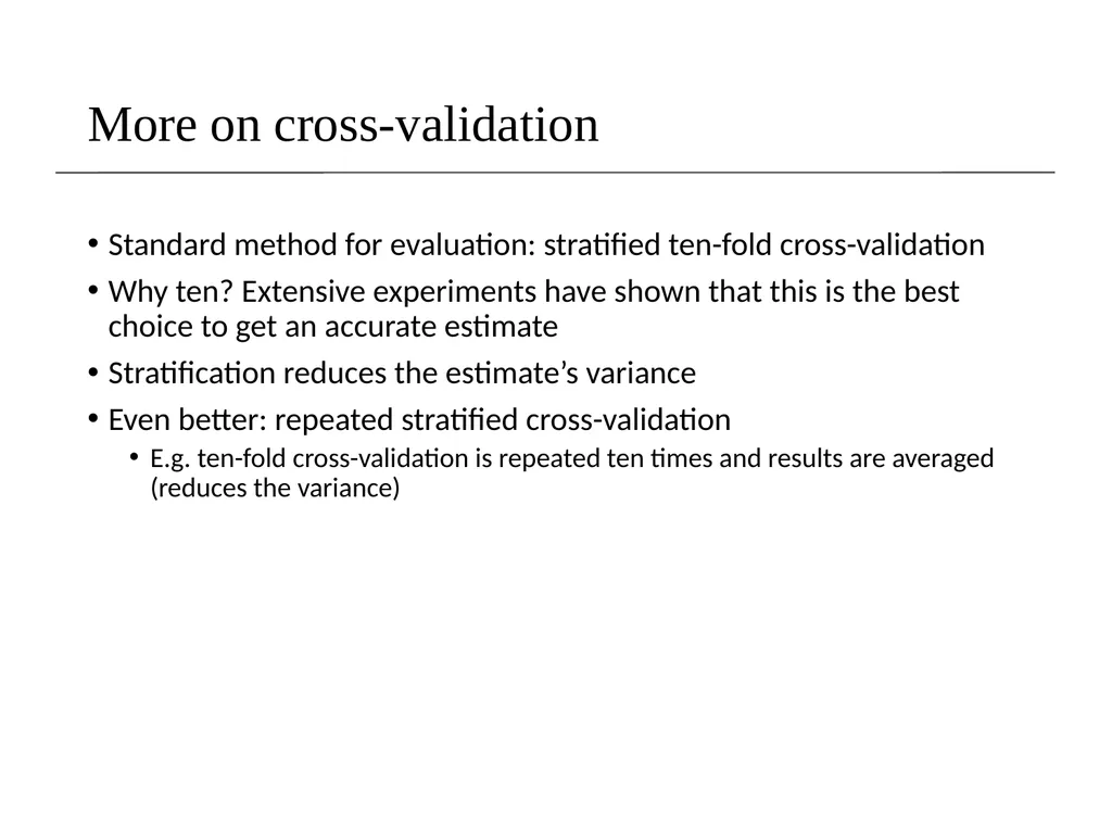
slide16. More on cross-validation Standard method for evaluation: stratified ten-fold cross-validation
Why ten? Extensive experiments have shown that this is the best choice to get an accurate estimate
Stratification reduces the estimate’s variance
Even better: repeated stratified cross-validation
E.g. ten-fold cross-validation is repeated ten times and results are averaged (reduces the variance)<br>
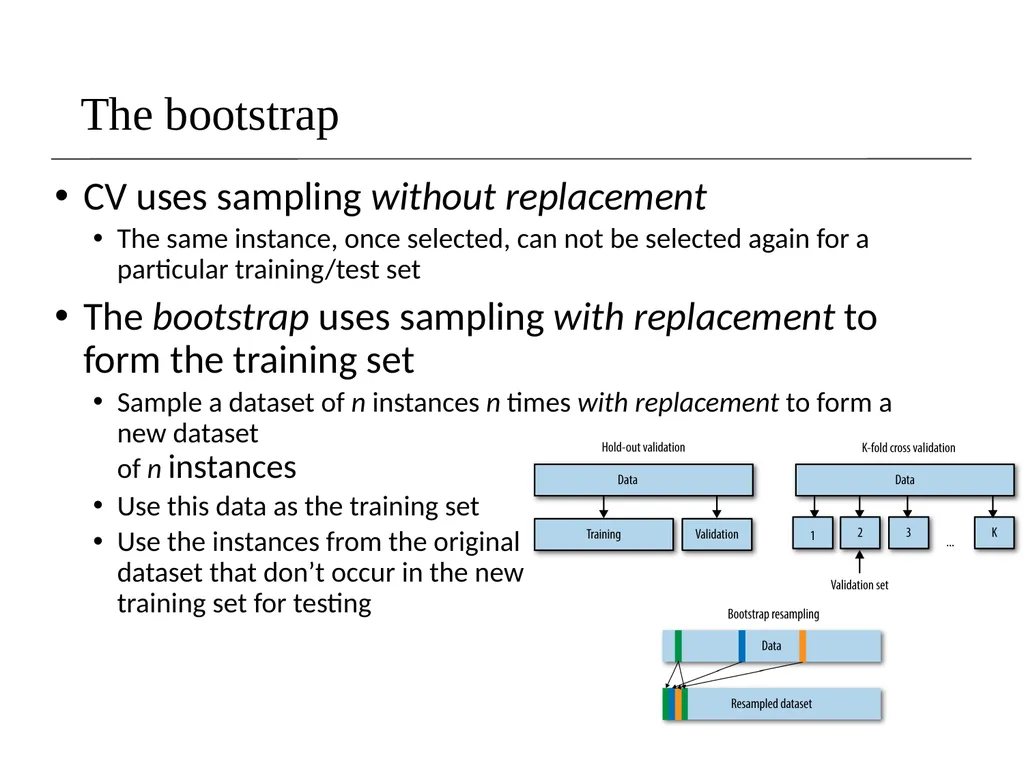
slide17. The bootstrap CV uses sampling without replacement
The same instance, once selected, can not be selected again for a particular training/test set
The bootstrap uses sampling with replacement to form the training set
Sample a dataset of n instances n times with replacement to form a new dataset of n instances
Use this data as the training set
Use the instances from the original dataset that don’t occur in the new training set for testing<br>
slide18. The bootstrap The bootstrap approach allows us to use a computer to mimic the process of obtaining new data sets, so that we can estimate the variability of our estimate without generating additional samples.
Rather than repeatedly obtaining independent data sets from the population, we instead obtain distinct data sets by repeatedly sampling observations from the original data set with replacement.
Each of these “bootstrap data sets” is created by sampling with replacement, and is the same size as our original dataset. As a result some observations may appear more than once in a given bootstrap data set and some not at all.<br>
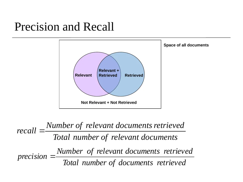
slide19. Precision and Recall Space of all documents<br>
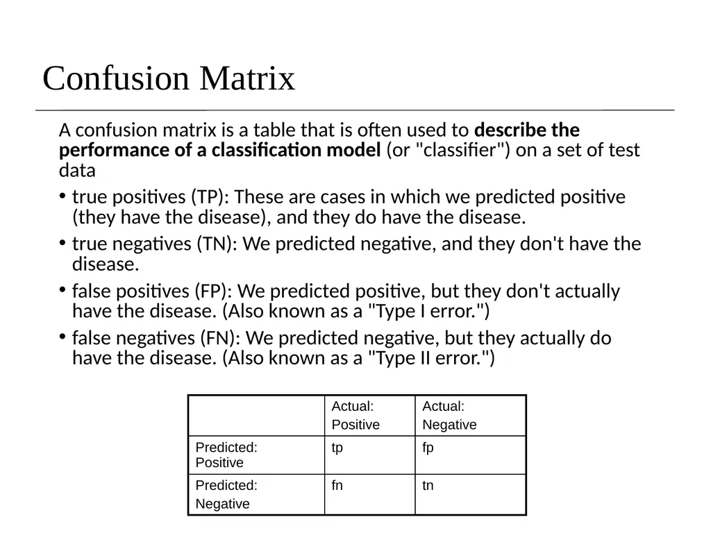
slide20. Confusion Matrix A confusion matrix is a table that is often used to describe the performance of a classification model (or "classifier") on a set of test data
true positives (TP): These are cases in which we predicted positive (they have the disease), and they do have the disease.
true negatives (TN): We predicted negative, and they don't have the disease.
false positives (FP): We predicted positive, but they don't actually have the disease. (Also known as a "Type I error.")
false negatives (FN): We predicted negative, but they actually do have the disease. (Also known as a "Type II error.")<br>
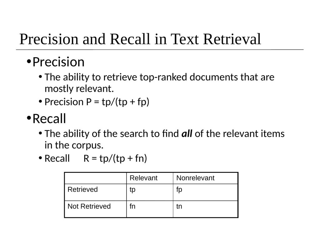
slide21. Precision and Recall in Text Retrieval Precision
The ability to retrieve top-ranked documents that are mostly relevant.
Precision P = tp/(tp + fp)
Recall
The ability of the search to find all of the relevant items in the corpus.
Recall R = tp/(tp + fn)<br>
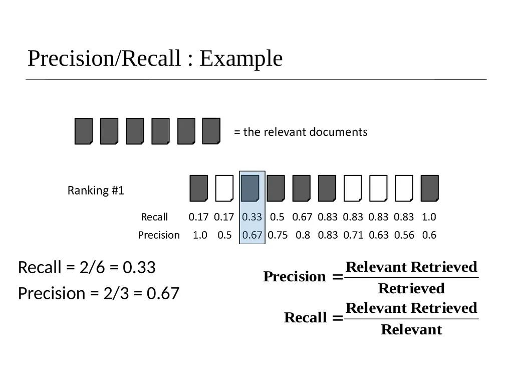
slide22. Precision/Recall : Example Recall = 2/6 = 0.33
Precision = 2/3 = 0.67<br>
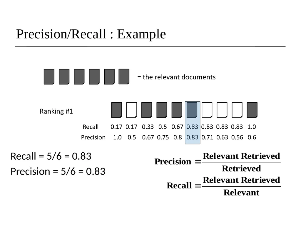
slide23. Recall = 5/6 = 0.83
Precision = 5/6 = 0.83 Precision/Recall : Example<br>
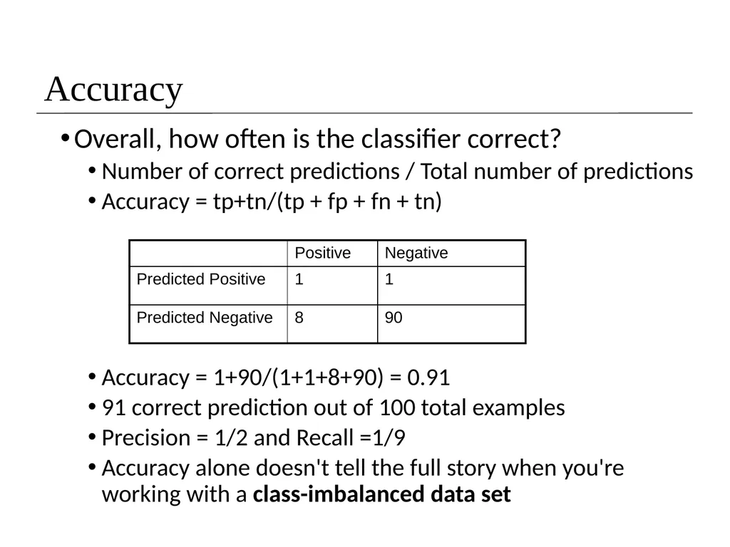
slide24. Accuracy Overall, how often is the classifier correct?
Number of correct predictions / Total number of predictions
Accuracy = tp+tn/(tp + fp + fn + tn)
Accuracy = 1+90/(1+1+8+90) = 0.91
91 correct prediction out of 100 total examples
Precision = 1/2 and Recall =1/9
Accuracy alone doesn't tell the full story when you're working with a class-imbalanced data set<br>
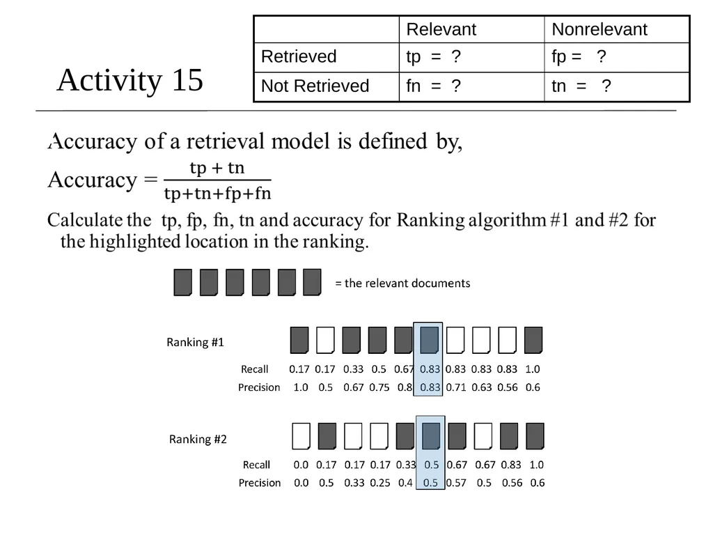
slide25. Activity 15<br>
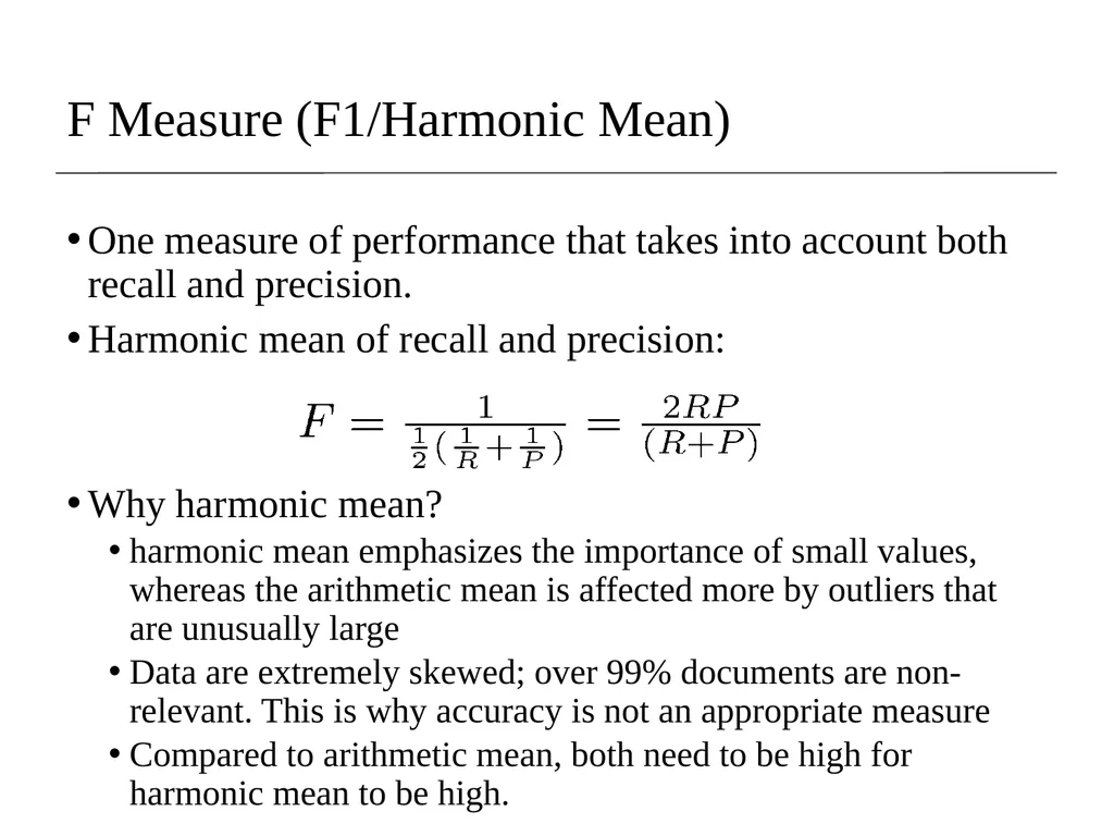
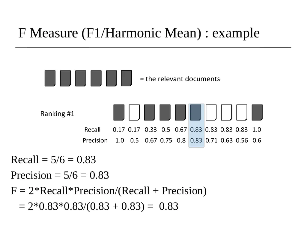
slide26. F Measure (F1/Harmonic Mean) One measure of performance that takes into account both recall and precision.
Harmonic mean of recall and precision:
Why harmonic mean?
harmonic mean emphasizes the importance of small values, whereas the arithmetic mean is affected more by outliers that are unusually large
Data are extremely skewed; over 99% documents are non-relevant. This is why accuracy is not an appropriate measure
Compared to arithmetic mean, both need to be high for harmonic mean to be high.<br>
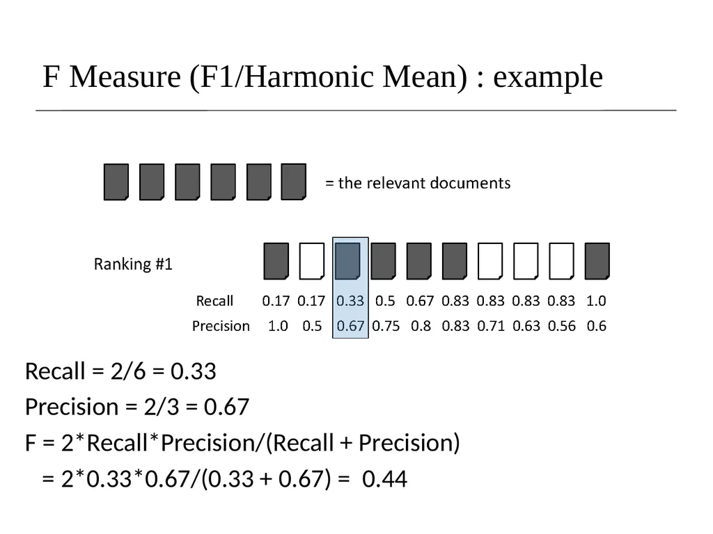
slide27. Recall = 2/6 = 0.33
Precision = 2/3 = 0.67
F = 2*Recall*Precision/(Recall + Precision)
= 2*0.33*0.67/(0.33 + 0.67) = 0.44 F Measure (F1/Harmonic Mean) : example<br>
slide28. Recall = 5/6 = 0.83
Precision = 5/6 = 0.83
F = 2*Recall*Precision/(Recall + Precision)
= 2*0.83*0.83/(0.83 + 0.83) = 0.83 F Measure (F1/Harmonic Mean) : example<br>
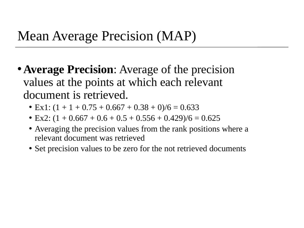
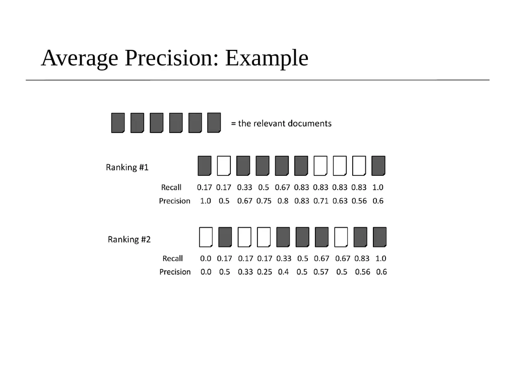
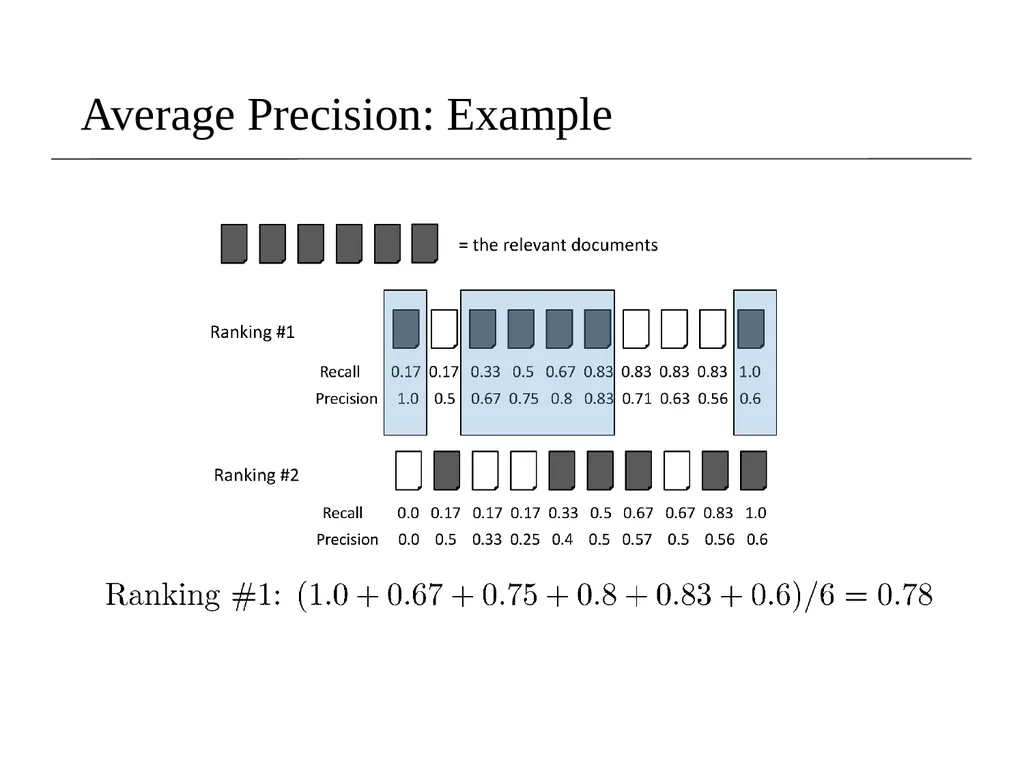
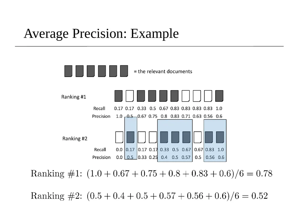
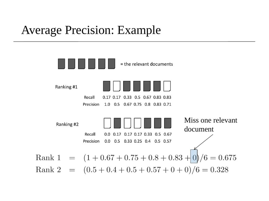
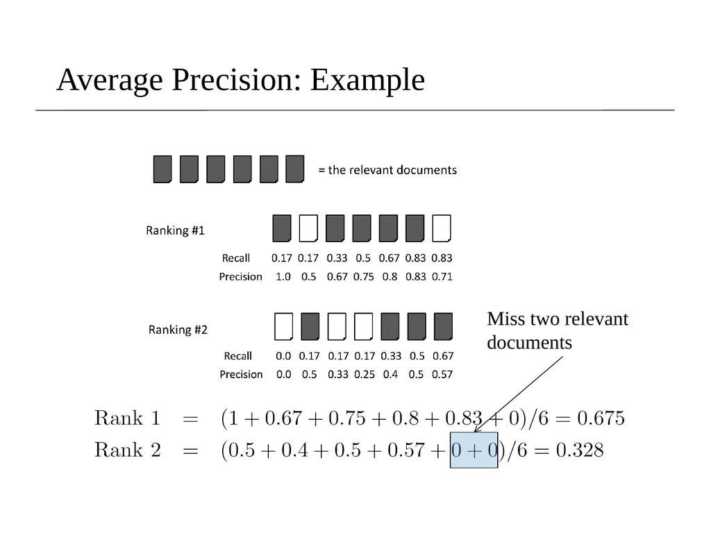
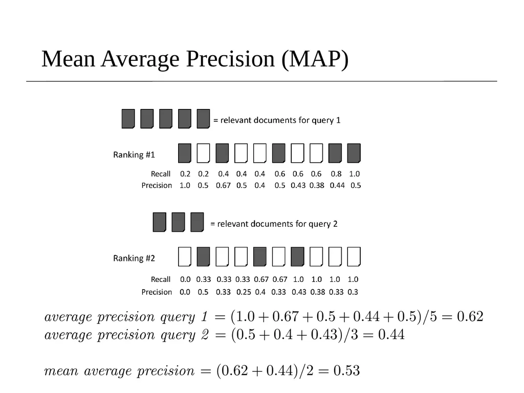
slide29. Mean Average Precision (MAP) Average Precision: Average of the precision values at the points at which each relevant document is retrieved.
Ex1: (1 + 1 + 0.75 + 0.667 + 0.38 + 0)/6 = 0.633
Ex2: (1 + 0.667 + 0.6 + 0.5 + 0.556 + 0.429)/6 = 0.625
Averaging the precision values from the rank positions where a relevant document was retrieved
Set precision values to be zero for the not retrieved documents<br>
slide30. Average Precision: Example<br>
slide31. Average Precision: Example<br>
slide32. Average Precision: Example<br>
slide33. Average Precision: Example Miss one relevant document<br>
slide34. Average Precision: Example Miss two relevant documents<br>
slide35. Mean Average Precision (MAP) Summarize rankings from multiple queries by averaging average precision
Most commonly used measure in research papers
Assumes user is interested in finding many relevant documents for each query
Requires many relevance judgments in text collection<br>
slide36. Mean Average Precision (MAP)<br>
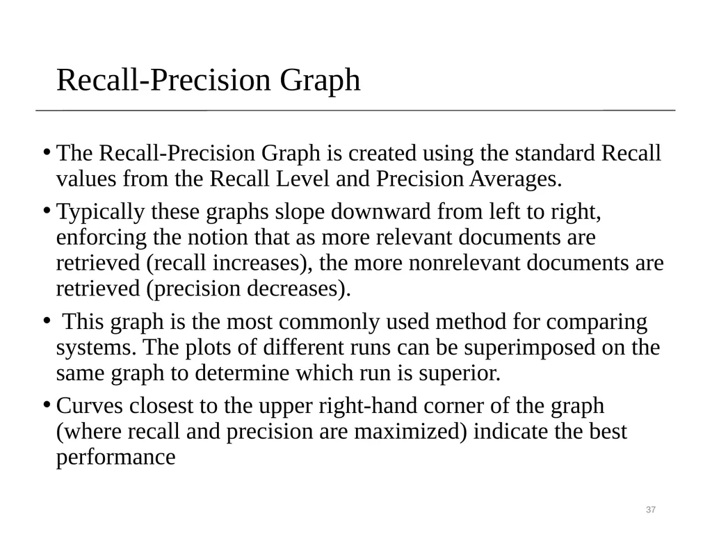
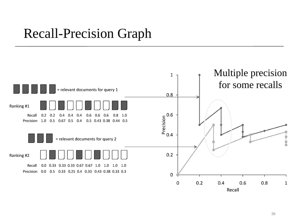
slide37. 37 Recall-Precision Graph The Recall-Precision Graph is created using the standard Recall values from the Recall Level and Precision Averages.
Typically these graphs slope downward from left to right, enforcing the notion that as more relevant documents are retrieved (recall increases), the more nonrelevant documents are retrieved (precision decreases).
This graph is the most commonly used method for comparing systems. The plots of different runs can be superimposed on the same graph to determine which run is superior.
Curves closest to the upper right-hand corner of the graph (where recall and precision are maximized) indicate the best performance<br>
slide38. 38 Recall-Precision Graph Multiple precision for some recalls<br>
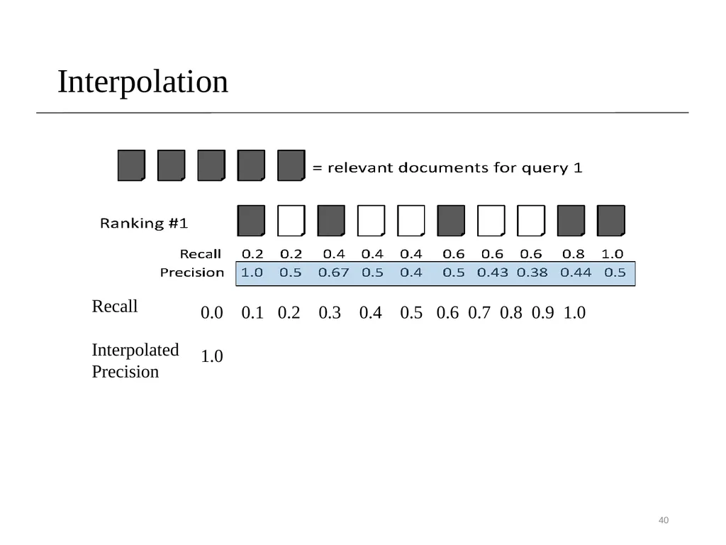
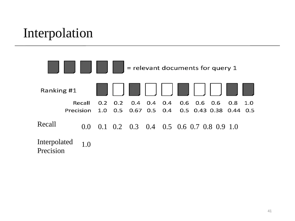
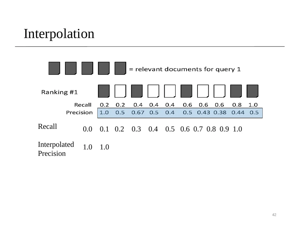
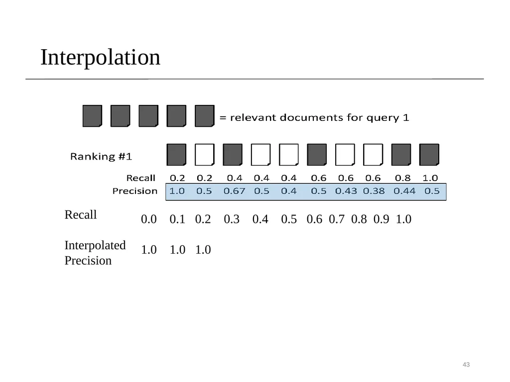
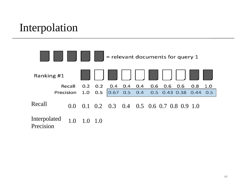
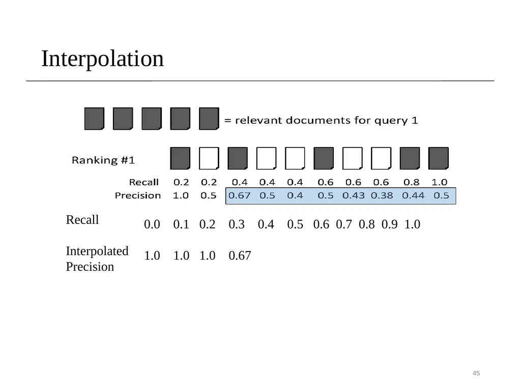
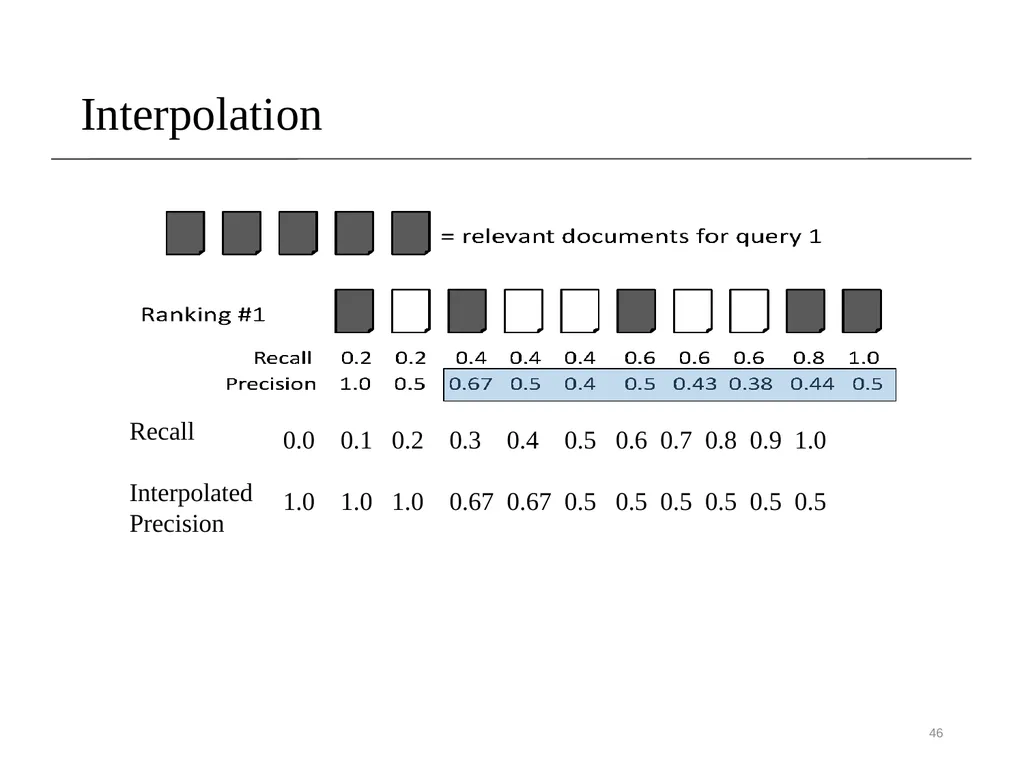
slide39. 39 Interpolation Defines precision at any recall level as the maximum precision observed in any recall-precision point at a higher recall level
produces a step function
defines precision at recall 0.0, 0.1……1.0<br>
slide40. Interpolation 40 Recall
Interpolated
Precision 0.0 0.1 0.2 0.3 0.4 0.5 0.6 0.7 0.8 0.9 1.0
1.0<br>
slide41. Interpolation 41 Recall
Interpolated
Precision 0.0 0.1 0.2 0.3 0.4 0.5 0.6 0.7 0.8 0.9 1.0
1.0<br>
slide42. Interpolation 42 Recall
Interpolated
Precision 0.0 0.1 0.2 0.3 0.4 0.5 0.6 0.7 0.8 0.9 1.0
1.0 1.0<br>
slide43. Interpolation 43 Recall
Interpolated
Precision 0.0 0.1 0.2 0.3 0.4 0.5 0.6 0.7 0.8 0.9 1.0
1.0 1.0 1.0<br>
slide44. Interpolation 44 Recall
Interpolated
Precision 0.0 0.1 0.2 0.3 0.4 0.5 0.6 0.7 0.8 0.9 1.0
1.0 1.0 1.0<br>
slide45. Interpolation 45 Recall
Interpolated
Precision 0.0 0.1 0.2 0.3 0.4 0.5 0.6 0.7 0.8 0.9 1.0
1.0 1.0 1.0 0.67<br>
slide46. Interpolation 46 Recall
Interpolated
Precision 0.0 0.1 0.2 0.3 0.4 0.5 0.6 0.7 0.8 0.9 1.0
1.0 1.0 1.0 0.67 0.67 0.5 0.5 0.5 0.5 0.5 0.5<br>
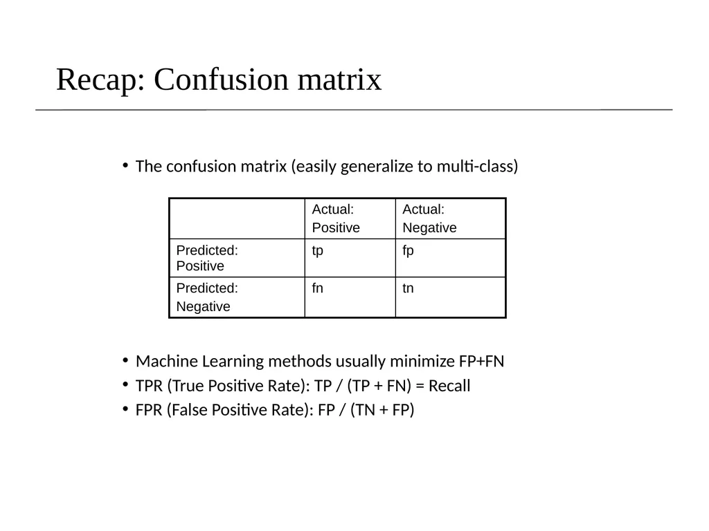
slide47. Recap: Confusion matrix The confusion matrix (easily generalize to multi-class)
Machine Learning methods usually minimize FP+FN
TPR (True Positive Rate): TP / (TP + FN) = Recall
FPR (False Positive Rate): FP / (TN + FP)<br>
slide48. ROC Curves A receiver operating characteristic curve, i.e. ROC curve, is a graphical plot that illustrates the diagnostic ability of a binary classifier system as its discrimination threshold is varied.
The diagnostic performance of a test, or the accuracy of a test to discriminate diseased cases from normal cases is evaluated using Receiver Operating Characteristic (ROC) curve analysis
A ROC Curve is a way to compare diagnostic tests. It is a plot of the true positive rate against the false positive rate.<br>
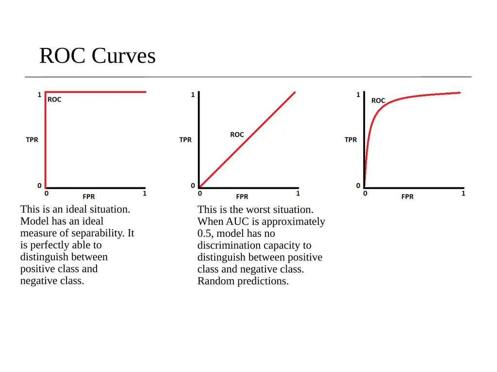
slide49. ROC Curves This is the worst situation. When AUC is approximately 0.5, model has no discrimination capacity to distinguish between positive class and negative class. Random predictions. This is an ideal situation. Model has an ideal measure of separability. It is perfectly able to distinguish between positive class and negative class.<br>
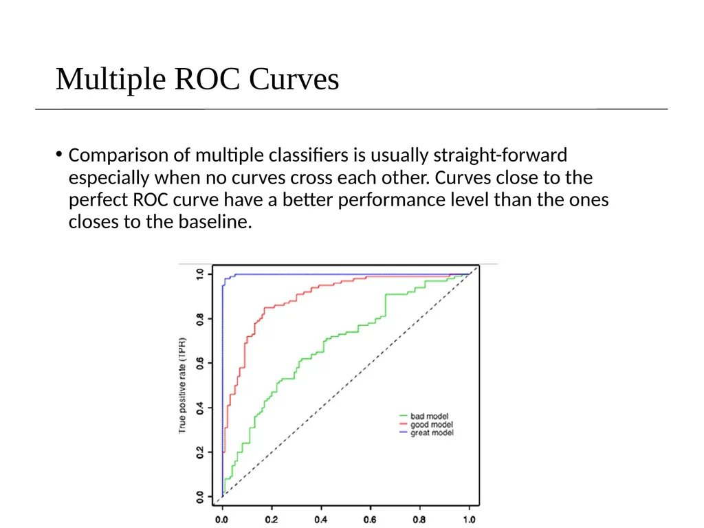
slide50. Multiple ROC Curves Comparison of multiple classifiers is usually straight-forward especially when no curves cross each other. Curves close to the perfect ROC curve have a better performance level than the ones closes to the baseline.<br>
slide51. PR Curves Vs ROC Curves Remember, a ROC curve represents a relation between sensitivity (Recall) and False Positive Rate (Not Precision).
ROC curve plot True Positive Rate Vs. False Positive Rate; Whereas, PR curve plot Precision Vs. Recall.
If your question is, "How well can this classifier be expected to perform in general, go with a ROC curve
If true negative is not much valuable to the problem, or negative examples are abundant. Then, PR-curve is typically more appropriate.
For example, if the class is highly imbalanced and positive samples are very rare, then use PR-curve.
How meaningful is a positive result from my classifier<br>
slide52. Cost-Sensitive Learning Learning to minimize the expected cost of misclassifications
Most classification learning algorithms attempt to minimize the expected number of misclassification errors
In many applications, different kinds of classification errors have different costs, so we need cost-sensitive methods<br>
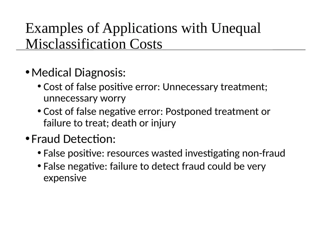
slide53. Examples of Applications with Unequal Misclassification Costs Medical Diagnosis:
Cost of false positive error: Unnecessary treatment; unnecessary worry
Cost of false negative error: Postponed treatment or failure to treat; death or injury
Fraud Detection:
False positive: resources wasted investigating non-fraud
False negative: failure to detect fraud could be very expensive<br>
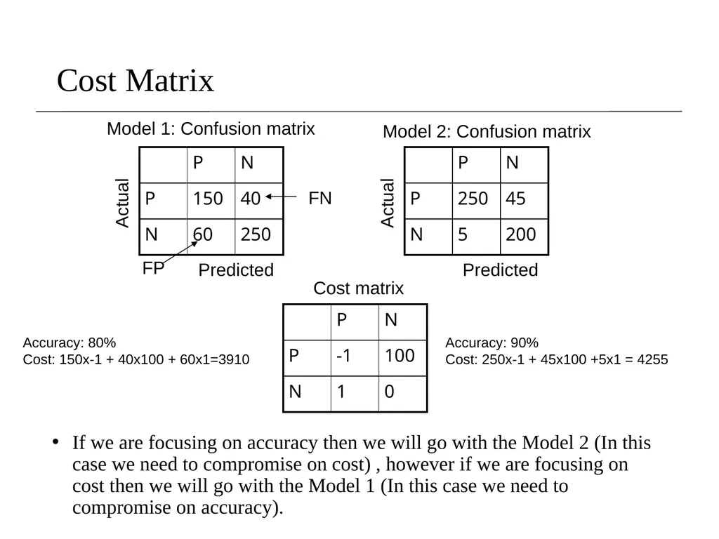
slide54. Cost Matrix Predicted Actual Model 1: Confusion matrix Cost matrix Predicted Actual Model 2: Confusion matrix FN FP Accuracy: 80%
Cost: 150x-1 + 40x100 + 60x1=3910 Accuracy: 90%
Cost: 250x-1 + 45x100 +5x1 = 4255 If we are focusing on accuracy then we will go with the Model 2 (In this case we need to compromise on cost) , however if we are focusing on cost then we will go with the Model 1 (In this case we need to compromise on accuracy).<br>
slide55. Significance Testing Also called “hypothesis testing”
Objective: to test a claim about parameter μ
Procedure:
State hypotheses H0 and Ha
Calculate test statistic
Convert test statistic to P-value and interpret
Consider significance level (optional)<br>
slide56. Hypotheses H0 (null hypothesis) claims “no difference”
Ha (alternative hypothesis) contradicts the null
Example: We test whether a population gained weight on average…
H0: no average weight gain in population Ha: H0 is wrong (i.e., “weight gain”)
Next collect data quantify the extent to which the data provides evidence against H0<br>
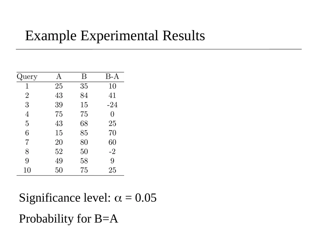
slide57. Significance Tests Given the results from a number of queries, how can we conclude that ranking algorithm B is better than algorithm A?
A significance test
null hypothesis: no difference between A and B
alternative hypothesis: B is better than A
the power of a test is the probability that the test will reject the null hypothesis correctly<br>
slide58. t-test The t test (also called Student’s T Test) compares two averages (means) and tells you if they are different from each other.
The t test also tells you how significant the differences are; In other words it lets you know if those differences could have happened by chance.<br>
slide59. t-test What are T-Values and P-values?
How big is “big enough”? Every t-value has a p-value to go with it.
A p-value is the probability that the results from your sample data occurred by chance.
P-values are from 0% to 100%. They are usually written as a decimal. For example, a p value of 5% is 0.05.
Low p-values are good; They indicate your data did not occur by chance.
For example, a p-value of .01 means there is only a 1% probability that the results from an experiment happened by chance. In most cases, a p-value of 0.05 (5%) is accepted or 95% confidence that experiment didn’t happen by a chance.<br>
slide60. Example Experimental Results Significance level: = 0.05
Probability for B=A<br>
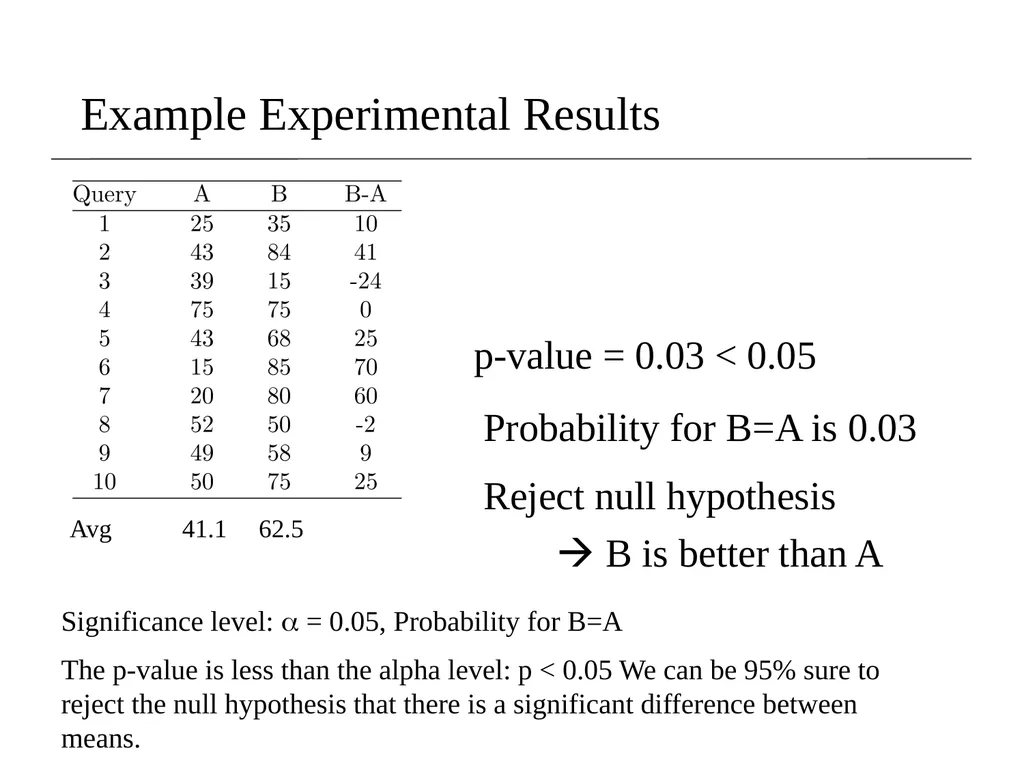
slide61. Example Experimental Results p-value = 0.03 < 0.05 Significance level: = 0.05, Probability for B=A
The p-value is less than the alpha level: p < 0.05 We can be 95% sure to reject the null hypothesis that there is a significant difference between means. B is better than A Probability for B=A is 0.03
Reject null hypothesis Avg 41.1 62.5<br>
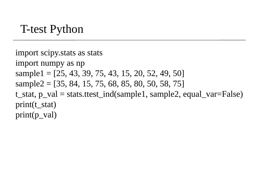
slide62. T-test Python import scipy.stats as stats
import numpy as np
sample1 = [25, 43, 39, 75, 43, 15, 20, 52, 49, 50]
sample2 = [35, 84, 15, 75, 68, 85, 80, 50, 58, 75]
t_stat, p_val = stats.ttest_ind(sample1, sample2, equal_var=False)
print(t_stat)
print(p_val)<br>
Cal Poly Pomona Credit for some of the slides in this lecture goes to Prof. Ray Mooney at UT Austin & Prof. Rong Jin at MSU CS 620 / DASC 600
Introduction to Data Science & Analytics<br>
slide2. Evaluation Evaluation = Process of judging the merit or worth of something
Evaluation is key to building effective and efficient Data Science systems
usually carried out in controlled experiments
online testing can also be done<br>
slide3. Why System Evaluation? There are many models/ algorithms/ systems, which one is the best?
What is the best component for:
similarity function (cosine, correlation,…)
Term selection (stopword removal, stemming…)
Term weighting (TF, TF-IDF,…)
How far down the list will a user need to look to find some/all relevant documents in text retrieval?<br>
slide4. Regression / classification models Predictive modeling / Supervised learning
A model is a specification of mathematical/probabilistic relationships that exist between different variables
The goal is usually to use existing data to develop models that we can use to predict outcomes for new data, such as
Predicting whether an email message is spam or not
Predicting whether a credit card transaction is fraudulent
Predicting which advertisement a shopper is most likely to click on
Predicting which football team is going to win the Super Bowl
Predicting stock price of a given company
Predicting number of buyers of a certain product
Predicting user ratings of a new movie
Predicting the grade of a disease Nominal
(categorical with
No particular order) Continuous / ordinal<br>
slide5. Performance evaluation How predictive is the model we learned?
For regression, usually R2 or MSE
For classification, many options (discuss later today)
Accuracy can be used, with caution
Performance on the training data (data used to build models) is not a good indicator of performance on future data
Q: Why?
A: Because new data will probably not be exactly the same as the training data!<br>
slide6. Overfitting vs underfitting Underfitting Overfitting High bias, low variance Low bias, high variance Increase # of features or complexity of model Get more training data, or reduce # of features or complexity of model Overfitting – fitting the training data too precisely - usually leads to poor results on new data
Underfitting – model does not fit training data well<br>
slide7. Evaluation on “LARGE” data If many (thousands) of examples are available, then how can we evaluate our model?
A simple evaluation is sufficient
Randomly split data into training and test sets (e.g. 2/3 for train, 1/3 for test)
For classification, make sure training and testing have similar distribution of class labels
Build a model using the train set and evaluate it using the test set.<br>
slide8. Model Evaluation Step 1: Split data into train and test sets Results Known 0 3 2 5 1 THE PAST Training set Testing set<br>
slide9. Model Evaluation Step 2: Build a model on a training set Results Known THE PAST Model Builder Testing set 0 3 2 5 1<br>
slide10. Model Evaluation Step 3: Evaluate on test set Predictions Results Known Training set Testing set Model Builder Evaluate 3
4
1
2 0 3 2 5 1<br>
slide11. A note on parameter tuning It is important that the test data is not used in any way to build the model
Some learning schemes operate in two stages:
Stage 1: builds the basic structure
Stage 2: optimizes parameter settings
The test data can’t be used for parameter tuning!
Proper procedure uses three sets: training data, validation data, and test data
Validation data is used to optimize parameters<br>
slide12. Evaluation on “small” data, 1 The holdout method reserves a certain amount for testing and uses the remainder for training
Usually: one third for testing, the rest for training
For “unbalanced” datasets, samples might not be representative
Few or none instances of some classes
Stratified sample: advanced version of balancing the data
Make sure that each class is represented with approximately equal proportions in both subsets<br>
slide13. Evaluation on “small” data, 2 What if we have a small data set?
The chosen 2/3 for training may not be representative.
The chosen 1/3 for testing may not be representative.<br>
slide14. Cross-validation Cross-validation more useful in small datasets
First step: data is split into k subsets of equal size
Second step: each subset in turn is used for testing and the remainder for training
This is called k-fold cross-validation
For classification, often the subsets are stratified before the cross-validation is performed
The error estimates are averaged to yield an overall error estimate<br>
slide15. 15 Cross-validation example: Break up data into groups of the same size
Hold aside one group for testing and use the rest to build model
Repeat Test<br>
slide16. More on cross-validation Standard method for evaluation: stratified ten-fold cross-validation
Why ten? Extensive experiments have shown that this is the best choice to get an accurate estimate
Stratification reduces the estimate’s variance
Even better: repeated stratified cross-validation
E.g. ten-fold cross-validation is repeated ten times and results are averaged (reduces the variance)<br>
slide17. The bootstrap CV uses sampling without replacement
The same instance, once selected, can not be selected again for a particular training/test set
The bootstrap uses sampling with replacement to form the training set
Sample a dataset of n instances n times with replacement to form a new dataset of n instances
Use this data as the training set
Use the instances from the original dataset that don’t occur in the new training set for testing<br>
slide18. The bootstrap The bootstrap approach allows us to use a computer to mimic the process of obtaining new data sets, so that we can estimate the variability of our estimate without generating additional samples.
Rather than repeatedly obtaining independent data sets from the population, we instead obtain distinct data sets by repeatedly sampling observations from the original data set with replacement.
Each of these “bootstrap data sets” is created by sampling with replacement, and is the same size as our original dataset. As a result some observations may appear more than once in a given bootstrap data set and some not at all.<br>
slide19. Precision and Recall Space of all documents<br>
slide20. Confusion Matrix A confusion matrix is a table that is often used to describe the performance of a classification model (or "classifier") on a set of test data
true positives (TP): These are cases in which we predicted positive (they have the disease), and they do have the disease.
true negatives (TN): We predicted negative, and they don't have the disease.
false positives (FP): We predicted positive, but they don't actually have the disease. (Also known as a "Type I error.")
false negatives (FN): We predicted negative, but they actually do have the disease. (Also known as a "Type II error.")<br>
slide21. Precision and Recall in Text Retrieval Precision
The ability to retrieve top-ranked documents that are mostly relevant.
Precision P = tp/(tp + fp)
Recall
The ability of the search to find all of the relevant items in the corpus.
Recall R = tp/(tp + fn)<br>
slide22. Precision/Recall : Example Recall = 2/6 = 0.33
Precision = 2/3 = 0.67<br>
slide23. Recall = 5/6 = 0.83
Precision = 5/6 = 0.83 Precision/Recall : Example<br>
slide24. Accuracy Overall, how often is the classifier correct?
Number of correct predictions / Total number of predictions
Accuracy = tp+tn/(tp + fp + fn + tn)
Accuracy = 1+90/(1+1+8+90) = 0.91
91 correct prediction out of 100 total examples
Precision = 1/2 and Recall =1/9
Accuracy alone doesn't tell the full story when you're working with a class-imbalanced data set<br>
slide25. Activity 15<br>
slide26. F Measure (F1/Harmonic Mean) One measure of performance that takes into account both recall and precision.
Harmonic mean of recall and precision:
Why harmonic mean?
harmonic mean emphasizes the importance of small values, whereas the arithmetic mean is affected more by outliers that are unusually large
Data are extremely skewed; over 99% documents are non-relevant. This is why accuracy is not an appropriate measure
Compared to arithmetic mean, both need to be high for harmonic mean to be high.<br>
slide27. Recall = 2/6 = 0.33
Precision = 2/3 = 0.67
F = 2*Recall*Precision/(Recall + Precision)
= 2*0.33*0.67/(0.33 + 0.67) = 0.44 F Measure (F1/Harmonic Mean) : example<br>
slide28. Recall = 5/6 = 0.83
Precision = 5/6 = 0.83
F = 2*Recall*Precision/(Recall + Precision)
= 2*0.83*0.83/(0.83 + 0.83) = 0.83 F Measure (F1/Harmonic Mean) : example<br>
slide29. Mean Average Precision (MAP) Average Precision: Average of the precision values at the points at which each relevant document is retrieved.
Ex1: (1 + 1 + 0.75 + 0.667 + 0.38 + 0)/6 = 0.633
Ex2: (1 + 0.667 + 0.6 + 0.5 + 0.556 + 0.429)/6 = 0.625
Averaging the precision values from the rank positions where a relevant document was retrieved
Set precision values to be zero for the not retrieved documents<br>
slide30. Average Precision: Example<br>
slide31. Average Precision: Example<br>
slide32. Average Precision: Example<br>
slide33. Average Precision: Example Miss one relevant document<br>
slide34. Average Precision: Example Miss two relevant documents<br>
slide35. Mean Average Precision (MAP) Summarize rankings from multiple queries by averaging average precision
Most commonly used measure in research papers
Assumes user is interested in finding many relevant documents for each query
Requires many relevance judgments in text collection<br>
slide36. Mean Average Precision (MAP)<br>
slide37. 37 Recall-Precision Graph The Recall-Precision Graph is created using the standard Recall values from the Recall Level and Precision Averages.
Typically these graphs slope downward from left to right, enforcing the notion that as more relevant documents are retrieved (recall increases), the more nonrelevant documents are retrieved (precision decreases).
This graph is the most commonly used method for comparing systems. The plots of different runs can be superimposed on the same graph to determine which run is superior.
Curves closest to the upper right-hand corner of the graph (where recall and precision are maximized) indicate the best performance<br>
slide38. 38 Recall-Precision Graph Multiple precision for some recalls<br>
slide39. 39 Interpolation Defines precision at any recall level as the maximum precision observed in any recall-precision point at a higher recall level
produces a step function
defines precision at recall 0.0, 0.1……1.0<br>
slide40. Interpolation 40 Recall
Interpolated
Precision 0.0 0.1 0.2 0.3 0.4 0.5 0.6 0.7 0.8 0.9 1.0
1.0<br>
slide41. Interpolation 41 Recall
Interpolated
Precision 0.0 0.1 0.2 0.3 0.4 0.5 0.6 0.7 0.8 0.9 1.0
1.0<br>
slide42. Interpolation 42 Recall
Interpolated
Precision 0.0 0.1 0.2 0.3 0.4 0.5 0.6 0.7 0.8 0.9 1.0
1.0 1.0<br>
slide43. Interpolation 43 Recall
Interpolated
Precision 0.0 0.1 0.2 0.3 0.4 0.5 0.6 0.7 0.8 0.9 1.0
1.0 1.0 1.0<br>
slide44. Interpolation 44 Recall
Interpolated
Precision 0.0 0.1 0.2 0.3 0.4 0.5 0.6 0.7 0.8 0.9 1.0
1.0 1.0 1.0<br>
slide45. Interpolation 45 Recall
Interpolated
Precision 0.0 0.1 0.2 0.3 0.4 0.5 0.6 0.7 0.8 0.9 1.0
1.0 1.0 1.0 0.67<br>
slide46. Interpolation 46 Recall
Interpolated
Precision 0.0 0.1 0.2 0.3 0.4 0.5 0.6 0.7 0.8 0.9 1.0
1.0 1.0 1.0 0.67 0.67 0.5 0.5 0.5 0.5 0.5 0.5<br>
slide47. Recap: Confusion matrix The confusion matrix (easily generalize to multi-class)
Machine Learning methods usually minimize FP+FN
TPR (True Positive Rate): TP / (TP + FN) = Recall
FPR (False Positive Rate): FP / (TN + FP)<br>
slide48. ROC Curves A receiver operating characteristic curve, i.e. ROC curve, is a graphical plot that illustrates the diagnostic ability of a binary classifier system as its discrimination threshold is varied.
The diagnostic performance of a test, or the accuracy of a test to discriminate diseased cases from normal cases is evaluated using Receiver Operating Characteristic (ROC) curve analysis
A ROC Curve is a way to compare diagnostic tests. It is a plot of the true positive rate against the false positive rate.<br>
slide49. ROC Curves This is the worst situation. When AUC is approximately 0.5, model has no discrimination capacity to distinguish between positive class and negative class. Random predictions. This is an ideal situation. Model has an ideal measure of separability. It is perfectly able to distinguish between positive class and negative class.<br>
slide50. Multiple ROC Curves Comparison of multiple classifiers is usually straight-forward especially when no curves cross each other. Curves close to the perfect ROC curve have a better performance level than the ones closes to the baseline.<br>
slide51. PR Curves Vs ROC Curves Remember, a ROC curve represents a relation between sensitivity (Recall) and False Positive Rate (Not Precision).
ROC curve plot True Positive Rate Vs. False Positive Rate; Whereas, PR curve plot Precision Vs. Recall.
If your question is, "How well can this classifier be expected to perform in general, go with a ROC curve
If true negative is not much valuable to the problem, or negative examples are abundant. Then, PR-curve is typically more appropriate.
For example, if the class is highly imbalanced and positive samples are very rare, then use PR-curve.
How meaningful is a positive result from my classifier<br>
slide52. Cost-Sensitive Learning Learning to minimize the expected cost of misclassifications
Most classification learning algorithms attempt to minimize the expected number of misclassification errors
In many applications, different kinds of classification errors have different costs, so we need cost-sensitive methods<br>
slide53. Examples of Applications with Unequal Misclassification Costs Medical Diagnosis:
Cost of false positive error: Unnecessary treatment; unnecessary worry
Cost of false negative error: Postponed treatment or failure to treat; death or injury
Fraud Detection:
False positive: resources wasted investigating non-fraud
False negative: failure to detect fraud could be very expensive<br>
slide54. Cost Matrix Predicted Actual Model 1: Confusion matrix Cost matrix Predicted Actual Model 2: Confusion matrix FN FP Accuracy: 80%
Cost: 150x-1 + 40x100 + 60x1=3910 Accuracy: 90%
Cost: 250x-1 + 45x100 +5x1 = 4255 If we are focusing on accuracy then we will go with the Model 2 (In this case we need to compromise on cost) , however if we are focusing on cost then we will go with the Model 1 (In this case we need to compromise on accuracy).<br>
slide55. Significance Testing Also called “hypothesis testing”
Objective: to test a claim about parameter μ
Procedure:
State hypotheses H0 and Ha
Calculate test statistic
Convert test statistic to P-value and interpret
Consider significance level (optional)<br>
slide56. Hypotheses H0 (null hypothesis) claims “no difference”
Ha (alternative hypothesis) contradicts the null
Example: We test whether a population gained weight on average…
H0: no average weight gain in population Ha: H0 is wrong (i.e., “weight gain”)
Next collect data quantify the extent to which the data provides evidence against H0<br>
slide57. Significance Tests Given the results from a number of queries, how can we conclude that ranking algorithm B is better than algorithm A?
A significance test
null hypothesis: no difference between A and B
alternative hypothesis: B is better than A
the power of a test is the probability that the test will reject the null hypothesis correctly<br>
slide58. t-test The t test (also called Student’s T Test) compares two averages (means) and tells you if they are different from each other.
The t test also tells you how significant the differences are; In other words it lets you know if those differences could have happened by chance.<br>
slide59. t-test What are T-Values and P-values?
How big is “big enough”? Every t-value has a p-value to go with it.
A p-value is the probability that the results from your sample data occurred by chance.
P-values are from 0% to 100%. They are usually written as a decimal. For example, a p value of 5% is 0.05.
Low p-values are good; They indicate your data did not occur by chance.
For example, a p-value of .01 means there is only a 1% probability that the results from an experiment happened by chance. In most cases, a p-value of 0.05 (5%) is accepted or 95% confidence that experiment didn’t happen by a chance.<br>
slide60. Example Experimental Results Significance level: = 0.05
Probability for B=A<br>
slide61. Example Experimental Results p-value = 0.03 < 0.05 Significance level: = 0.05, Probability for B=A
The p-value is less than the alpha level: p < 0.05 We can be 95% sure to reject the null hypothesis that there is a significant difference between means. B is better than A Probability for B=A is 0.03
Reject null hypothesis Avg 41.1 62.5<br>
slide62. T-test Python import scipy.stats as stats
import numpy as np
sample1 = [25, 43, 39, 75, 43, 15, 20, 52, 49, 50]
sample2 = [35, 84, 15, 75, 68, 85, 80, 50, 58, 75]
t_stat, p_val = stats.ttest_ind(sample1, sample2, equal_var=False)
print(t_stat)
print(p_val)<br>