Machine Learning: Methodology Chapter 18.1-18.3

lindy-dunigan

Published 2026-01-24 · 29 slides · 0 views

↓ Download

Machine Learning: Methodology Chapter 18.1-18.3

Machine Learning: Methodology Chapter 18.1-18.3 - slide 1 of 29

Machine Learning: Methodology Chapter 18.1-18.3 - slide 2 of 29

Machine Learning: Methodology Chapter 18.1-18.3 - slide 3 of 29

Machine Learning: Methodology Chapter 18.1-18.3 - slide 4 of 29

Machine Learning: Methodology Chapter 18.1-18.3 - slide 5 of 29

Machine Learning: Methodology Chapter 18.1-18.3 - slide 6 of 29

Machine Learning: Methodology Chapter 18.1-18.3 - slide 7 of 29

Machine Learning: Methodology Chapter 18.1-18.3 - slide 8 of 29

Machine Learning: Methodology Chapter 18.1-18.3 - slide 9 of 29

Machine Learning: Methodology Chapter 18.1-18.3 - slide 10 of 29

Machine Learning: Methodology Chapter 18.1-18.3 - slide 11 of 29

Machine Learning: Methodology Chapter 18.1-18.3 - slide 12 of 29

Machine Learning: Methodology Chapter 18.1-18.3 - slide 13 of 29

Machine Learning: Methodology Chapter 18.1-18.3 - slide 14 of 29

Machine Learning: Methodology Chapter 18.1-18.3 - slide 15 of 29

Machine Learning: Methodology Chapter 18.1-18.3 - slide 16 of 29

Machine Learning: Methodology Chapter 18.1-18.3 - slide 17 of 29

Machine Learning: Methodology Chapter 18.1-18.3 - slide 18 of 29

Machine Learning: Methodology Chapter 18.1-18.3 - slide 19 of 29

Machine Learning: Methodology Chapter 18.1-18.3 - slide 20 of 29

Machine Learning: Methodology Chapter 18.1-18.3 - slide 21 of 29

Machine Learning: Methodology Chapter 18.1-18.3 - slide 22 of 29

Machine Learning: Methodology Chapter 18.1-18.3 - slide 23 of 29

Machine Learning: Methodology Chapter 18.1-18.3 - slide 24 of 29

Machine Learning: Methodology Chapter 18.1-18.3 - slide 25 of 29

Machine Learning: Methodology Chapter 18.1-18.3 - slide 26 of 29

Machine Learning: Methodology Chapter 18.1-18.3 - slide 27 of 29

Machine Learning: Methodology Chapter 18.1-18.3 - slide 28 of 29

Machine Learning: Methodology Chapter 18.1-18.3 - slide 29 of 29

Description

Machine Learning: Methodology Chapter 18.1-18.3 http:archive.ics.uci.eduml 233 data sets http:archive.ics.uci.edumldatasetsZoo Zoo data animal name: string hair: Boolean feathers: Boolean eggs: Boolean milk: Boolean airborne:

Download this presentation From Below

"Machine Learning: Methodology Chapter 18.1-18.3" is the property of its rightful owner. Permission is granted to download and print the materials on this website for personal, non-commercial use only, and to display it on your personal computer provided you do not modify the materials and that you retain all copyright notices contained in the materials. By downloading content from our website, you accept the terms of this agreement.

Presentation Transcript

Machine Learning: Methodology Chapter 18.1-18.3

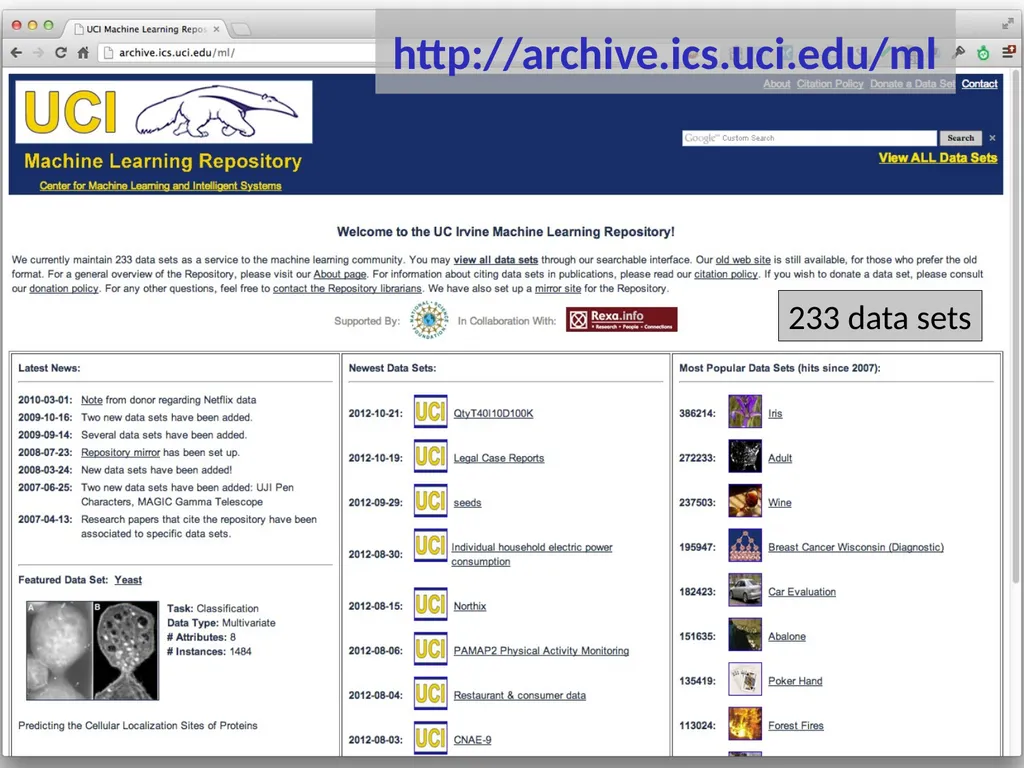
http://archive.ics.uci.edu/ml 233 data sets

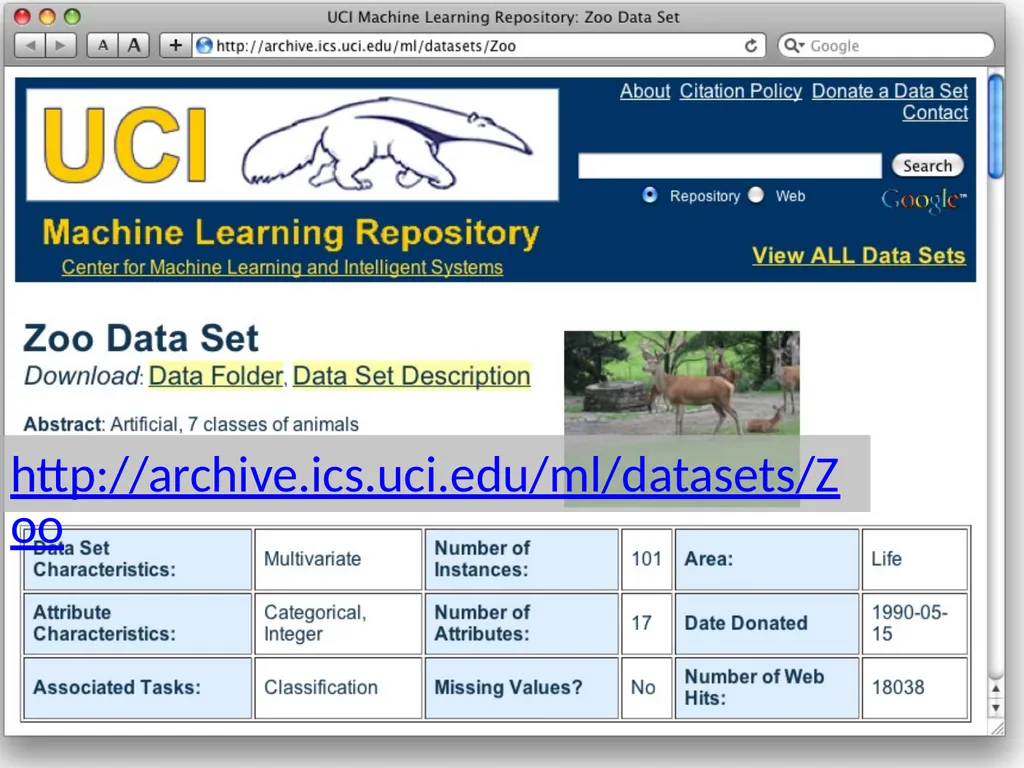
http://archive.ics.uci.edu/ml/datasets/Zoo

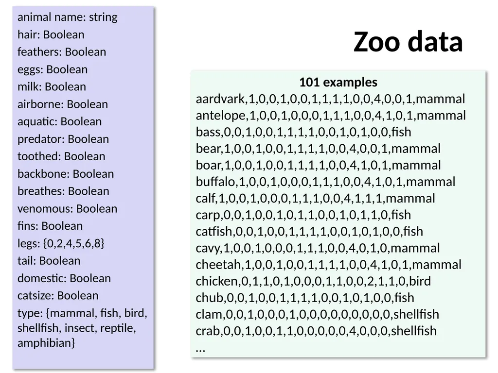
Zoo data animal name: string
hair: Boolean
feathers: Boolean
eggs: Boolean
milk: Boolean
airborne: Boolean
aquatic: Boolean
predator: Boolean
toothed: Boolean
backbone: Boolean
breathes: Boolean
venomous: Boolean
fins: Boolean
legs: {0,2,4,5,6,8}
tail: Boolean
domestic: Boolean
catsize: Boolean
type: {mammal, fish, bird, shellfish, insect, reptile, amphibian} 101 examples
aardvark,1,0,0,1,0,0,1,1,1,1,0,0,4,0,0,1,mammal
antelope,1,0,0,1,0,0,0,1,1,1,0,0,4,1,0,1,mammal
bass,0,0,1,0,0,1,1,1,1,0,0,1,0,1,0,0,fish
bear,1,0,0,1,0,0,1,1,1,1,0,0,4,0,0,1,mammal
boar,1,0,0,1,0,0,1,1,1,1,0,0,4,1,0,1,mammal
buffalo,1,0,0,1,0,0,0,1,1,1,0,0,4,1,0,1,mammal
calf,1,0,0,1,0,0,0,1,1,1,0,0,4,1,1,1,mammal
carp,0,0,1,0,0,1,0,1,1,0,0,1,0,1,1,0,fish
catfish,0,0,1,0,0,1,1,1,1,0,0,1,0,1,0,0,fish
cavy,1,0,0,1,0,0,0,1,1,1,0,0,4,0,1,0,mammal
cheetah,1,0,0,1,0,0,1,1,1,1,0,0,4,1,0,1,mammal
chicken,0,1,1,0,1,0,0,0,1,1,0,0,2,1,1,0,bird
chub,0,0,1,0,0,1,1,1,1,0,0,1,0,1,0,0,fish
clam,0,0,1,0,0,0,1,0,0,0,0,0,0,0,0,0,shellfish
crab,0,0,1,0,0,1,1,0,0,0,0,0,4,0,0,0,shellfish
…

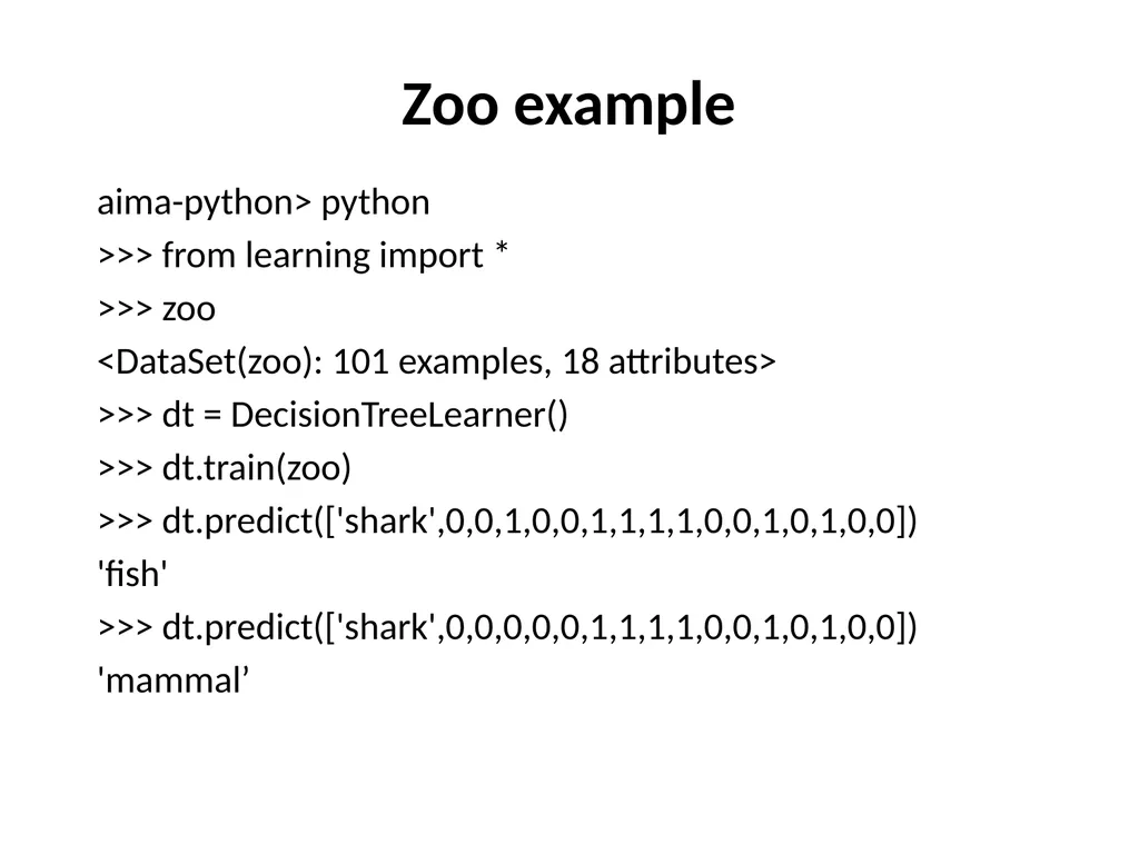
Zoo example aima-python> python
>>> from learning import *
>>> zoo
<DataSet(zoo): 101 examples, 18 attributes>
>>> dt = DecisionTreeLearner()
>>> dt.train(zoo)
>>> dt.predict(['shark',0,0,1,0,0,1,1,1,1,0,0,1,0,1,0,0])
'fish'
>>> dt.predict(['shark',0,0,0,0,0,1,1,1,1,0,0,1,0,1,0,0])
'mammal’

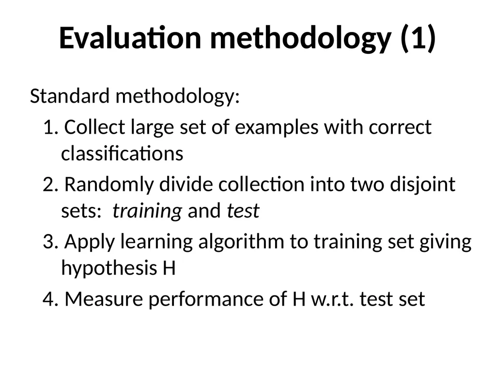
Evaluation methodology (1) Standard methodology:
1. Collect large set of examples with correct classifications
2. Randomly divide collection into two disjoint sets: training and test
3. Apply learning algorithm to training set giving hypothesis H
4. Measure performance of H w.r.t. test set

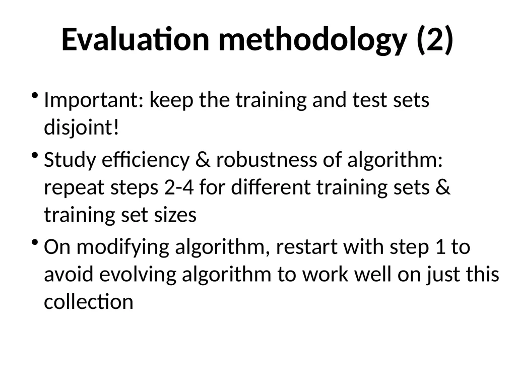
Evaluation methodology (2) Important: keep the training and test sets disjoint!
Study efficiency & robustness of algorithm: repeat steps 2-4 for different training sets & training set sizes
On modifying algorithm, restart with step 1 to avoid evolving algorithm to work well on just this collection

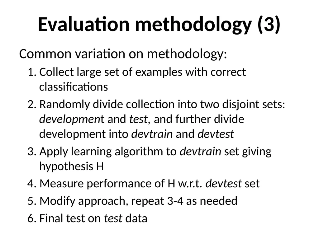
Evaluation methodology (3) Common variation on methodology:
1. Collect large set of examples with correct classifications
2. Randomly divide collection into two disjoint sets: development and test, and further divide development into devtrain and devtest
3. Apply learning algorithm to devtrain set giving hypothesis H
4. Measure performance of H w.r.t. devtest set
5. Modify approach, repeat 3-4 as needed
6. Final test on test data

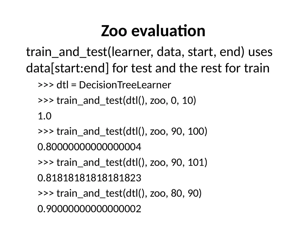
Zoo evaluation train_and_test(learner, data, start, end) uses data[start:end] for test and the rest for train
>>> dtl = DecisionTreeLearner
>>> train_and_test(dtl(), zoo, 0, 10)
1.0
>>> train_and_test(dtl(), zoo, 90, 100)
0.80000000000000004
>>> train_and_test(dtl(), zoo, 90, 101)
0.81818181818181823
>>> train_and_test(dtl(), zoo, 80, 90)
0.90000000000000002

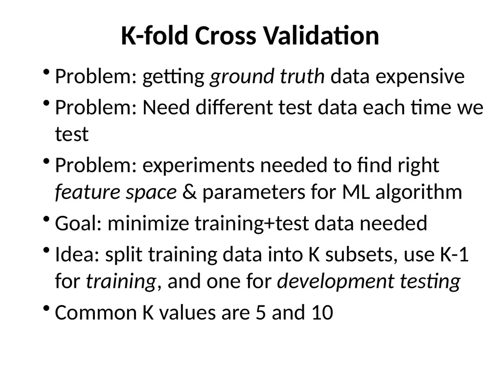
K-fold Cross Validation Problem: getting ground truth data expensive
Problem: Need different test data each time we test
Problem: experiments needed to find right feature space & parameters for ML algorithm
Goal: minimize training+test data needed
Idea: split training data into K subsets, use K-1 for training, and one for development testing
Common K values are 5 and 10

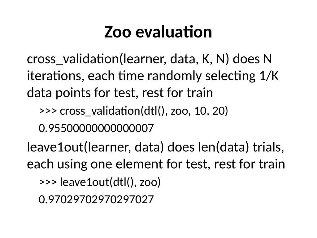
Zoo evaluation cross_validation(learner, data, K, N) does N iterations, each time randomly selecting 1/K data points for test, rest for train
>>> cross_validation(dtl(), zoo, 10, 20)
0.95500000000000007
leave1out(learner, data) does len(data) trials, each using one element for test, rest for train
>>> leave1out(dtl(), zoo)
0.97029702970297027

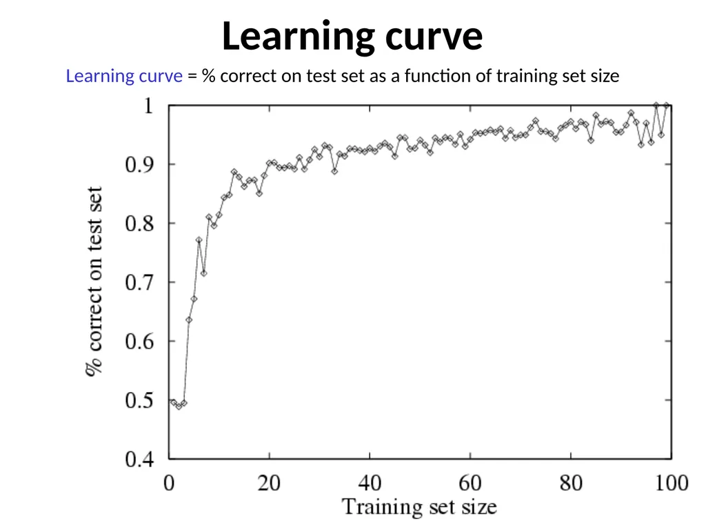
Learning curve Learning curve = % correct on test set as a function of training set size

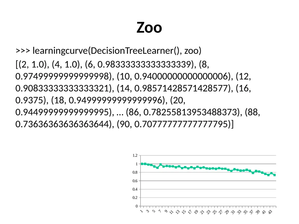
Zoo >>> learningcurve(DecisionTreeLearner(), zoo)
[(2, 1.0), (4, 1.0), (6, 0.98333333333333339), (8, 0.97499999999999998), (10, 0.94000000000000006), (12, 0.90833333333333321), (14, 0.98571428571428577), (16, 0.9375), (18, 0.94999999999999996), (20, 0.94499999999999995), … (86, 0.78255813953488373), (88, 0.73636363636363644), (90, 0.70777777777777795)]

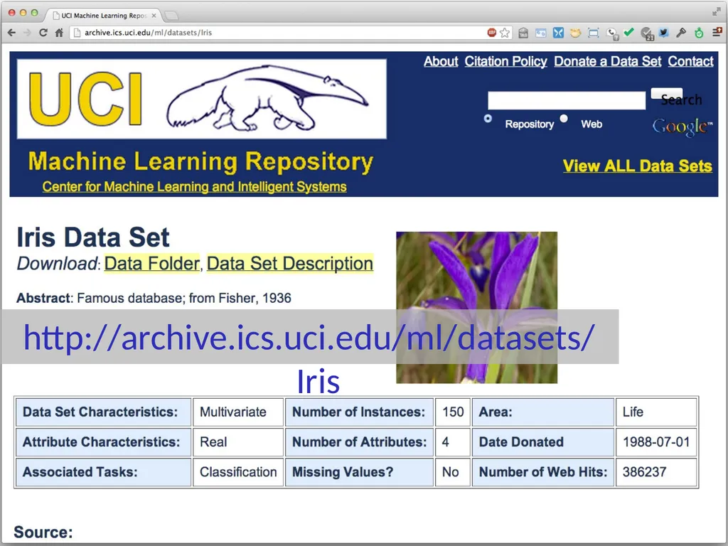
http://archive.ics.uci.edu/ml/datasets/Iris

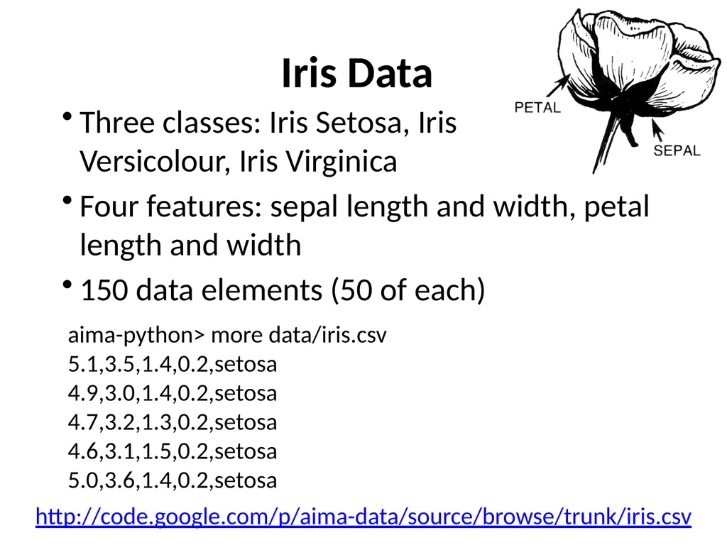
Iris Data Three classes: Iris Setosa, IrisVersicolour, Iris Virginica
Four features: sepal length and width, petal length and width
150 data elements (50 of each) aima-python> more data/iris.csv
5.1,3.5,1.4,0.2,setosa
4.9,3.0,1.4,0.2,setosa
4.7,3.2,1.3,0.2,setosa
4.6,3.1,1.5,0.2,setosa
5.0,3.6,1.4,0.2,setosa http://code.google.com/p/aima-data/source/browse/trunk/iris.csv

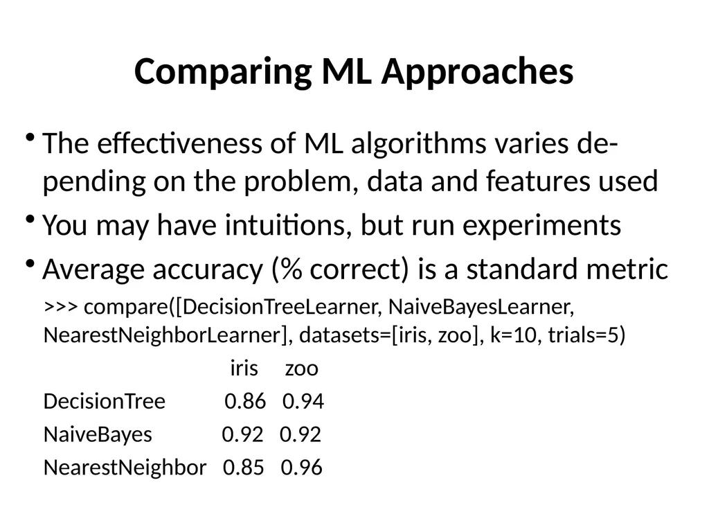
Comparing ML Approaches The effectiveness of ML algorithms varies de-pending on the problem, data and features used
You may have intuitions, but run experiments
Average accuracy (% correct) is a standard metric
>>> compare([DecisionTreeLearner, NaiveBayesLearner, NearestNeighborLearner], datasets=[iris, zoo], k=10, trials=5)
iris zoo
DecisionTree 0.86 0.94
NaiveBayes 0.92 0.92
NearestNeighbor 0.85 0.96

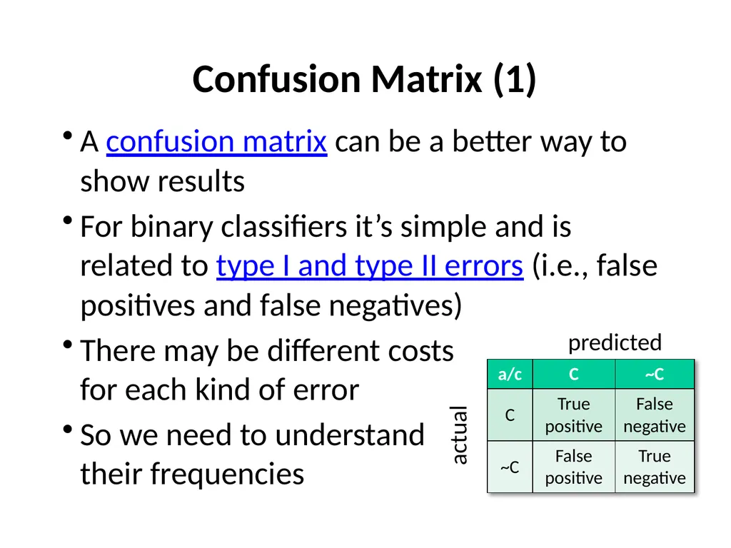
Confusion Matrix (1) A confusion matrix can be a better way to show results
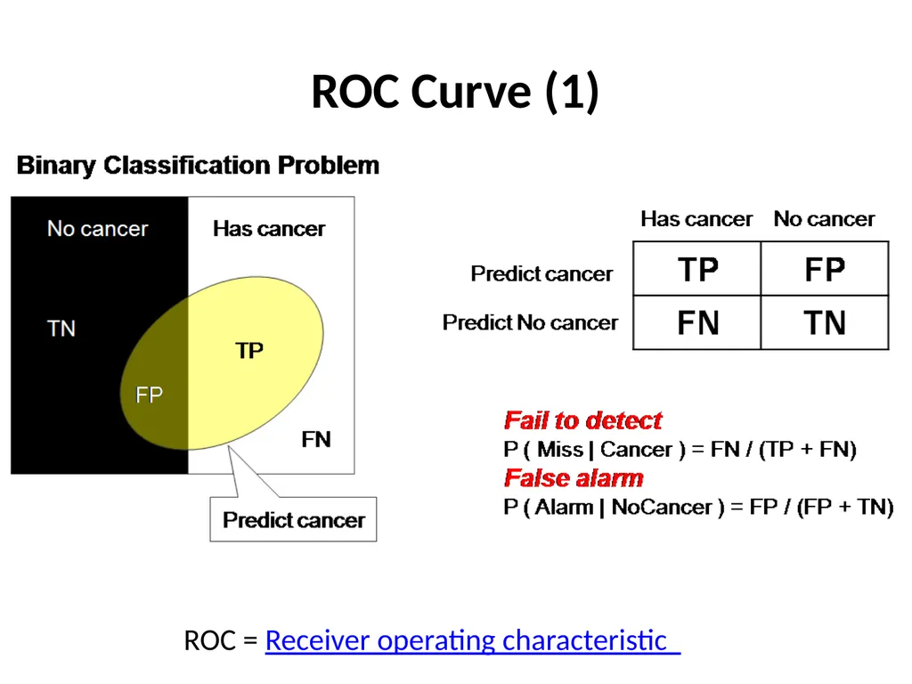
For binary classifiers it’s simple and is related to type I and type II errors (i.e., false positives and false negatives)
There may be different costsfor each kind of error
So we need to understandtheir frequencies predicted actual

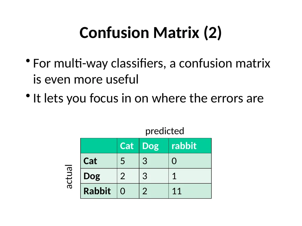
Confusion Matrix (2) For multi-way classifiers, a confusion matrix is even more useful
It lets you focus in on where the errors are predicted actual

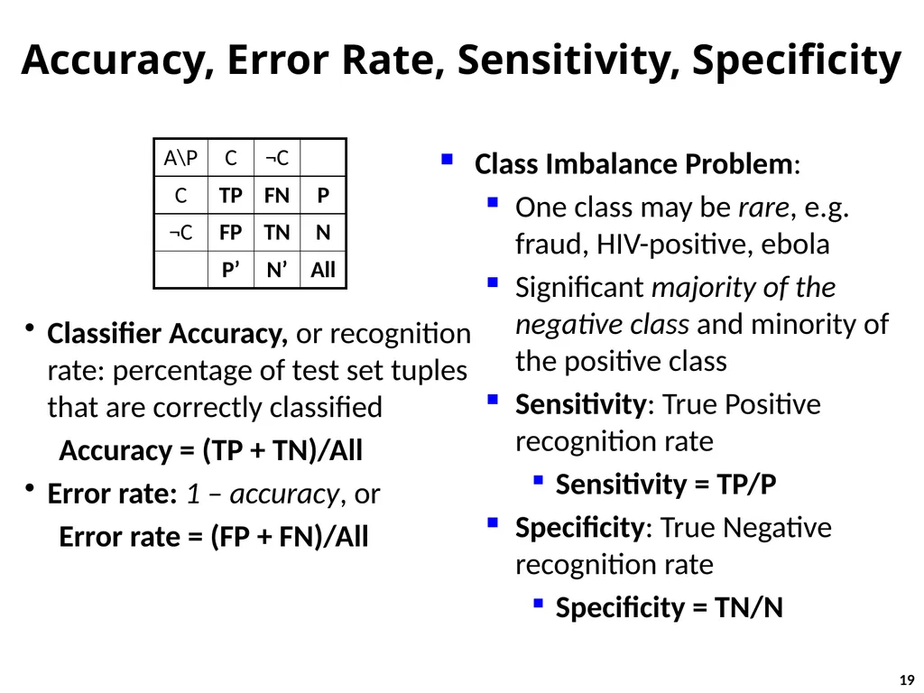
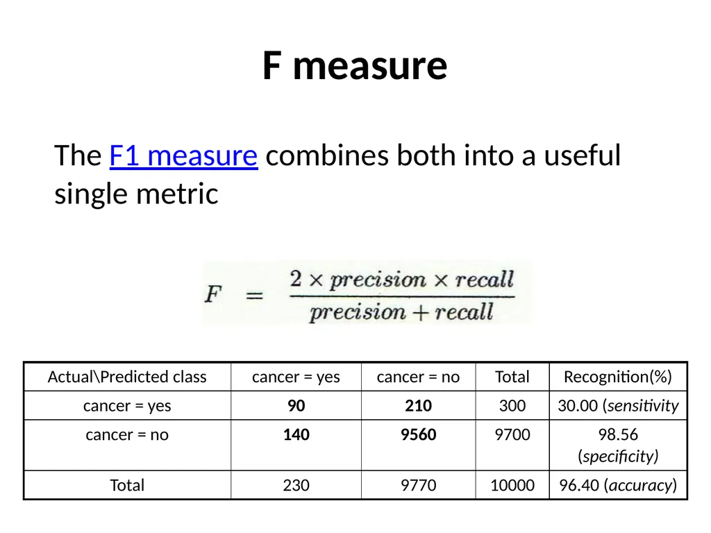
Accuracy, Error Rate, Sensitivity, Specificity Classifier Accuracy, or recognition rate: percentage of test set tuples that are correctly classified
Accuracy = (TP + TN)/All
Error rate: 1 – accuracy, or
Error rate = (FP + FN)/All Class Imbalance Problem:
One class may be rare, e.g. fraud, HIV-positive, ebola
Significant majority of the negative class and minority of the positive class
Sensitivity: True Positive recognition rate
Sensitivity = TP/P
Specificity: True Negative recognition rate
Specificity = TN/N 19

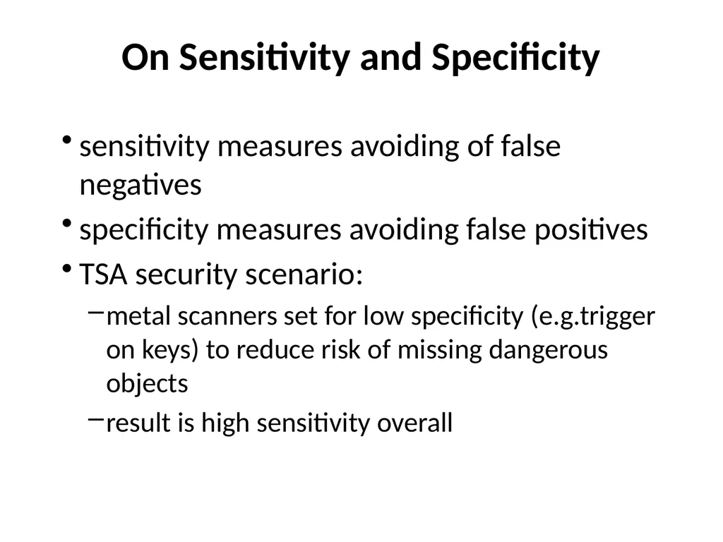
On Sensitivity and Specificity sensitivity measures avoiding of false negatives
specificity measures avoiding false positives
TSA security scenario:
metal scanners set for low specificity (e.g.trigger on keys) to reduce risk of missing dangerous objects
result is high sensitivity overall

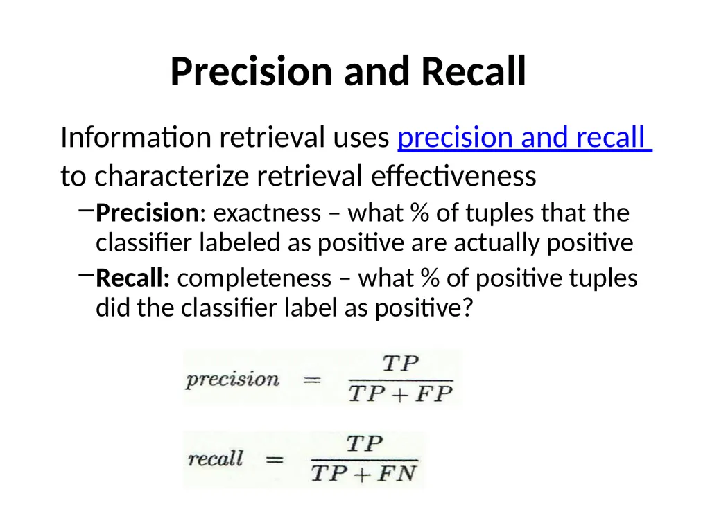
Precision and Recall Information retrieval uses precision and recall to characterize retrieval effectiveness
Precision: exactness – what % of tuples that the classifier labeled as positive are actually positive
Recall: completeness – what % of positive tuples did the classifier label as positive?

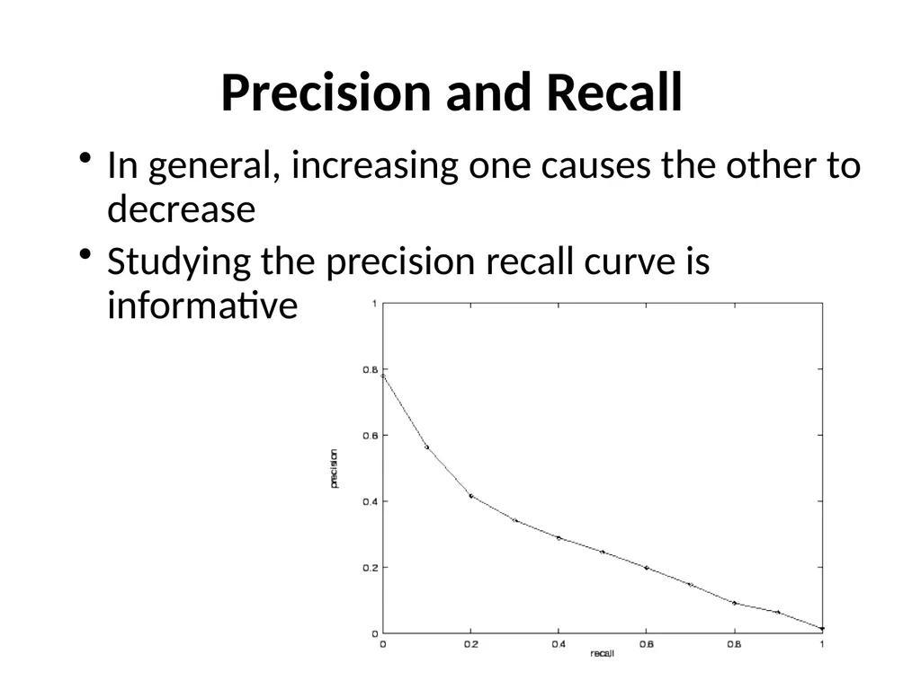
Precision and Recall In general, increasing one causes the other to decrease
Studying the precision recall curve is informative

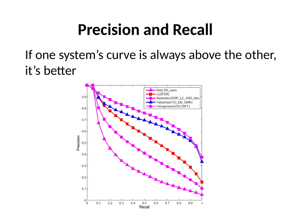
Precision and Recall If one system’s curve is always above the other, it’s better

F measure The F1 measure combines both into a useful single metric

ROC Curve (1) ROC = Receiver operating characteristic

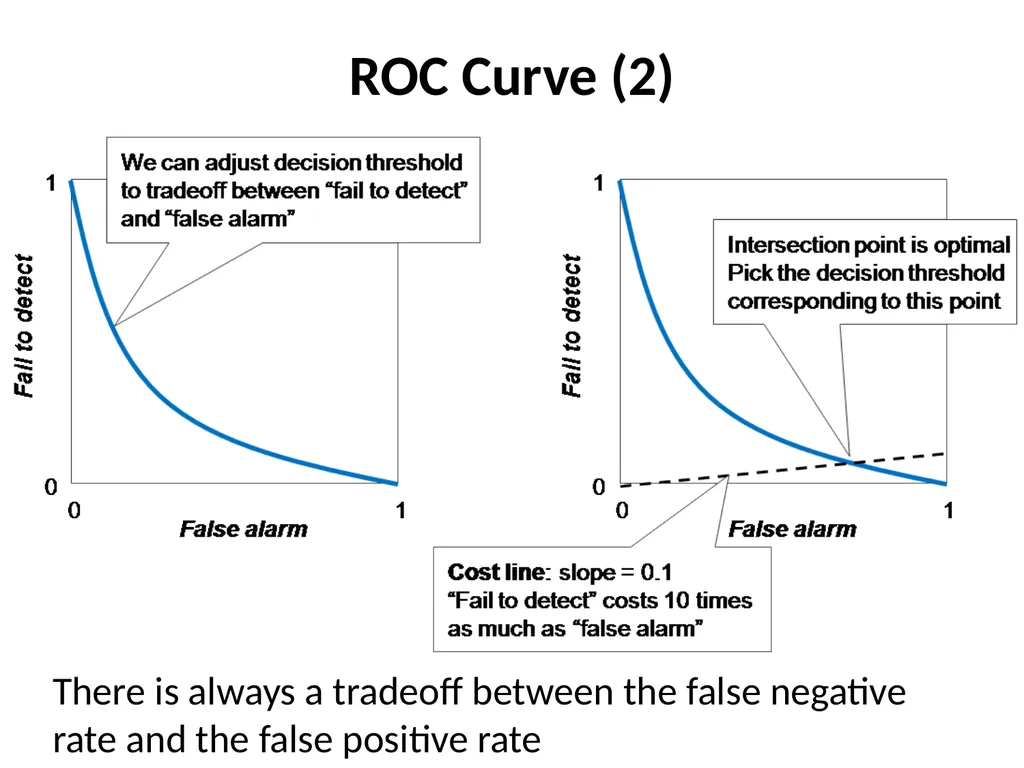
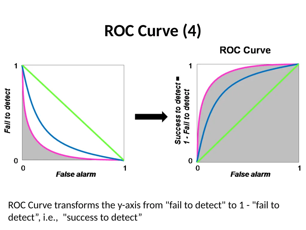
ROC Curve (2) There is always a tradeoff between the false negative rate and the false positive rate

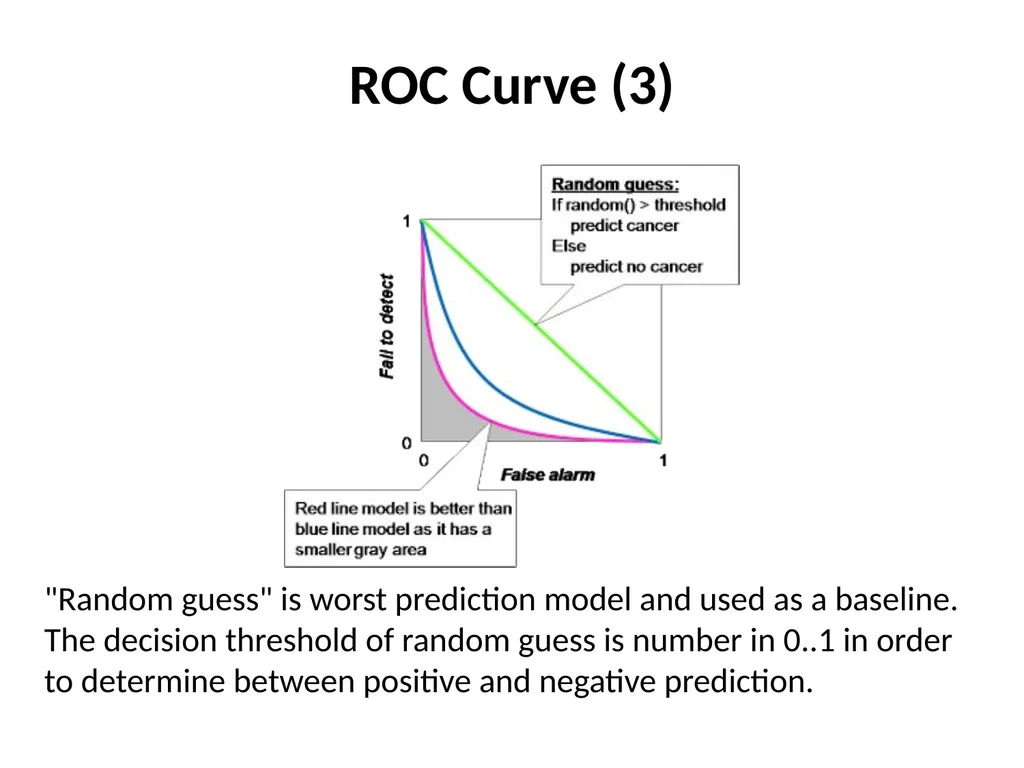
ROC Curve (3) "Random guess" is worst prediction model and used as a baseline. The decision threshold of random guess is number in 0..1 in order to determine between positive and negative prediction.

ROC Curve (4) ROC Curve transforms the y-axis from "fail to detect" to 1 - "fail to detect”, i.e., "success to detect”

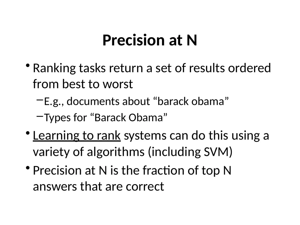
Precision at N Ranking tasks return a set of results ordered from best to worst
E.g., documents about “barack obama”
Types for “Barack Obama”
Learning to rank systems can do this using a variety of algorithms (including SVM)
Precision at N is the fraction of top N answers that are correct

Machine Learning: Methodology Chapter 18.1-18.3

Related Topics

Share

Embed code

Download this presentation From Below

Presentation Transcript