
Microsoft® Office Excel® 2007 Training Enter



Description: Microsoft Office Excel 2007 Training Enter formulas INLS261 Tools for Information Literacy Enter formulas Course contents Overview: Goodbye, calculator Lesson 1: Get started Lesson 2: Use cell references Lesson 3: Simplify formulas by
Related Topics
Download Presentation
"Microsoft® Office Excel® 2007 Training Enter" is the property of its rightful owner. Permission is granted to download and print the materials on this website for personal, non-commercial use only, and to display it on your personal computer provided you do not modify the materials and that you retain all copyright notices contained in the materials. By downloading content from our website, you accept the terms of this agreement.
Presentation Transcript
slide1. Microsoft® Office
Excel® 2007 Training Enter formulas INLS261 Tools for Information Literacy<br>
slide2. Enter formulas Course contents Overview: Goodbye, calculator
Lesson 1: Get started
Lesson 2: Use cell references
Lesson 3: Simplify formulas by using functions Each lesson includes a list of suggested tasks and a set of test questions. 2 November 2007 2<br>
slide3. Enter formulas Overview: Goodbye, calculator Excel is great for working with numbers and math. In this course you’ll learn how add, divide, multiply, and subtract by typing formulas into Excel worksheets.
You’ll also learn how to use simple formulas that automatically update their results when values change.
After picking up the techniques in this course, you’ll be able to put your calculator away for good. 2 November 2007 3<br>
slide4. Enter formulas Course goals Do math by typing simple formulas to add, divide, multiply, and subtract.
Use cell references in formulas, so that Excel can automatically update results when values change or when you copy formulas.
Use functions (prewritten formulas) to add up values, calculate averages, and find the smallest or largest value in a range of values. 2 November 2007 4<br>
slide5. Lesson 1 Get started<br>
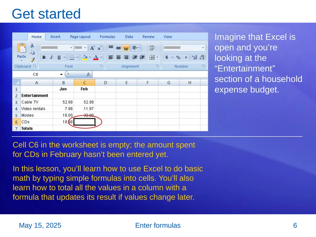
slide6. Enter formulas Get started Imagine that Excel is open and you’re looking at the “Entertainment” section of a household expense budget. Cell C6 in the worksheet is empty; the amount spent for CDs in February hasn’t been entered yet.
In this lesson, you’ll learn how to use Excel to do basic math by typing simple formulas into cells. You’ll also learn how to total all the values in a column with a formula that updates its result if values change later. 2 November 2007 6<br>
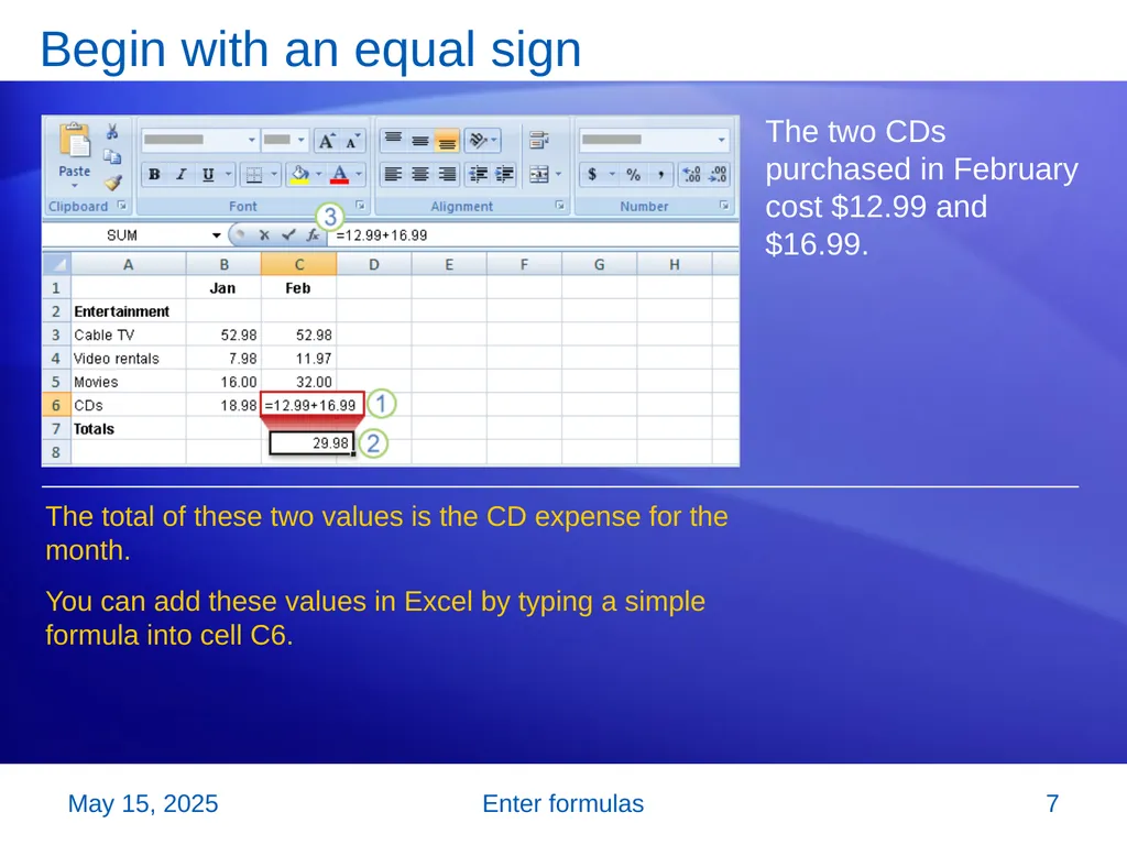
slide7. Enter formulas Begin with an equal sign The two CDs purchased in February cost $12.99 and $16.99. The total of these two values is the CD expense for the month.
You can add these values in Excel by typing a simple formula into cell C6. 2 November 2007 7<br>
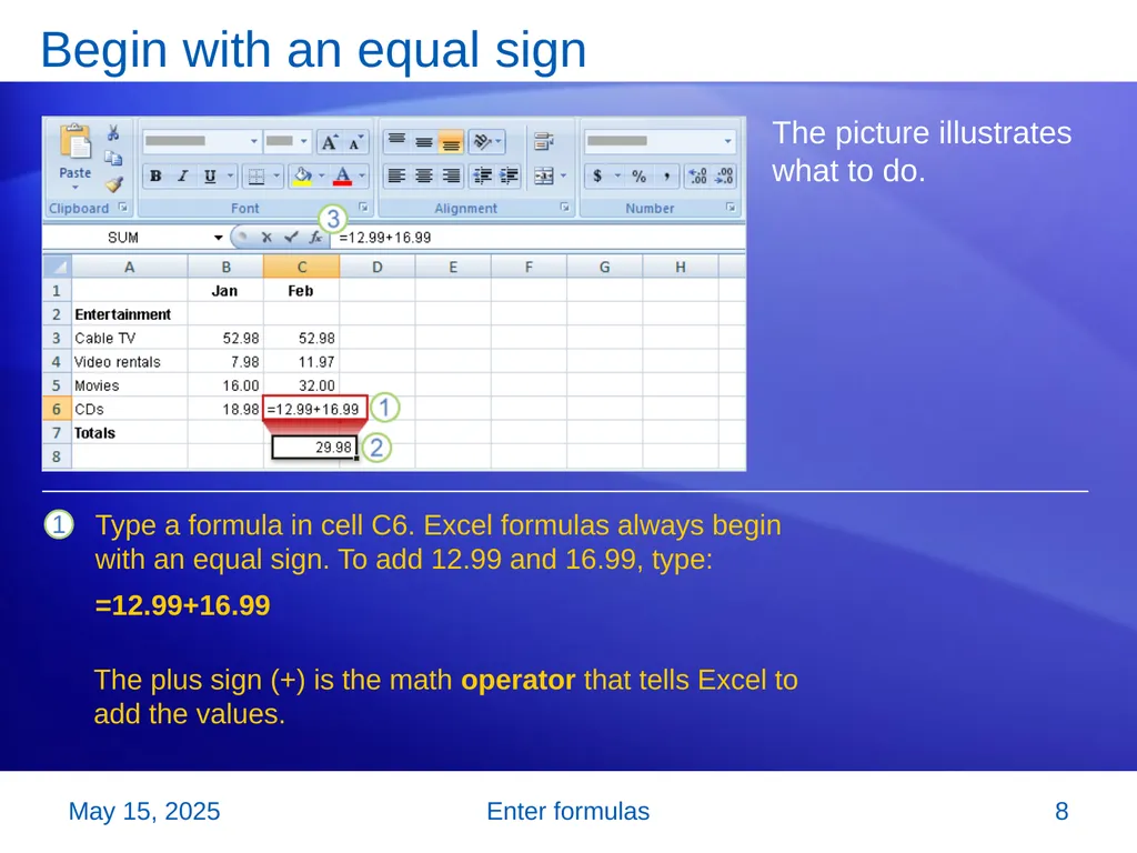
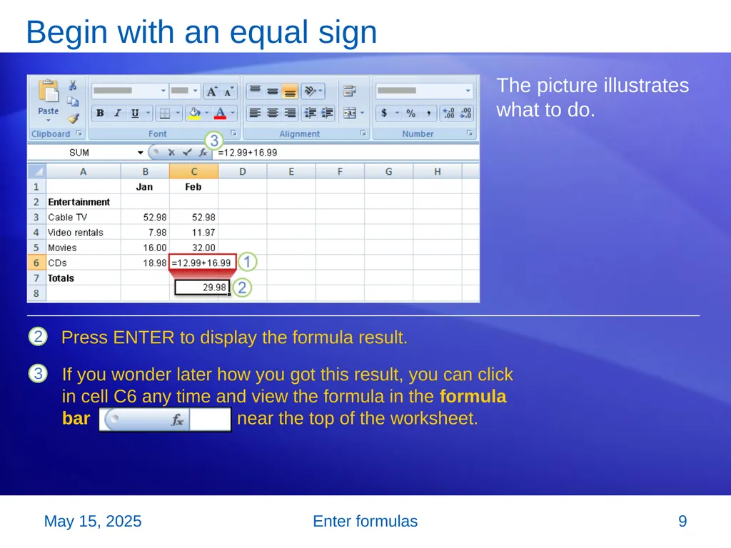
slide8. Enter formulas Begin with an equal sign The picture illustrates what to do. Type a formula in cell C6. Excel formulas always begin with an equal sign. To add 12.99 and 16.99, type:
=12.99+16.99 The plus sign (+) is the math operator that tells Excel to add the values. 2 November 2007 8<br>
slide9. Enter formulas Begin with an equal sign The picture illustrates what to do. Press ENTER to display the formula result. If you wonder later how you got this result, you can click in cell C6 any time and view the formula in the formula bar near the top of the worksheet. 2 November 2007 9<br>
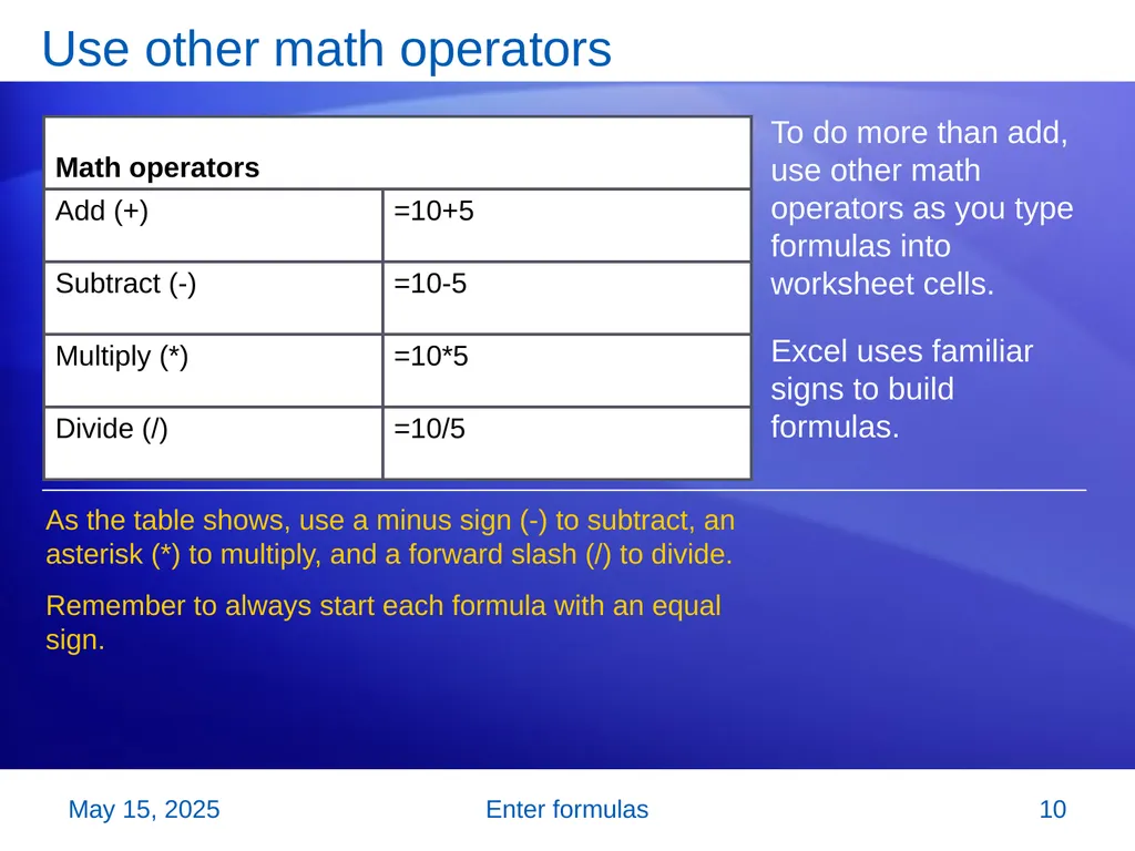
slide10. Enter formulas Use other math operators To do more than add, use other math operators as you type formulas into worksheet cells.
Excel uses familiar signs to build formulas. As the table shows, use a minus sign (-) to subtract, an asterisk (*) to multiply, and a forward slash (/) to divide.
Remember to always start each formula with an equal sign. 2 November 2007 10<br>
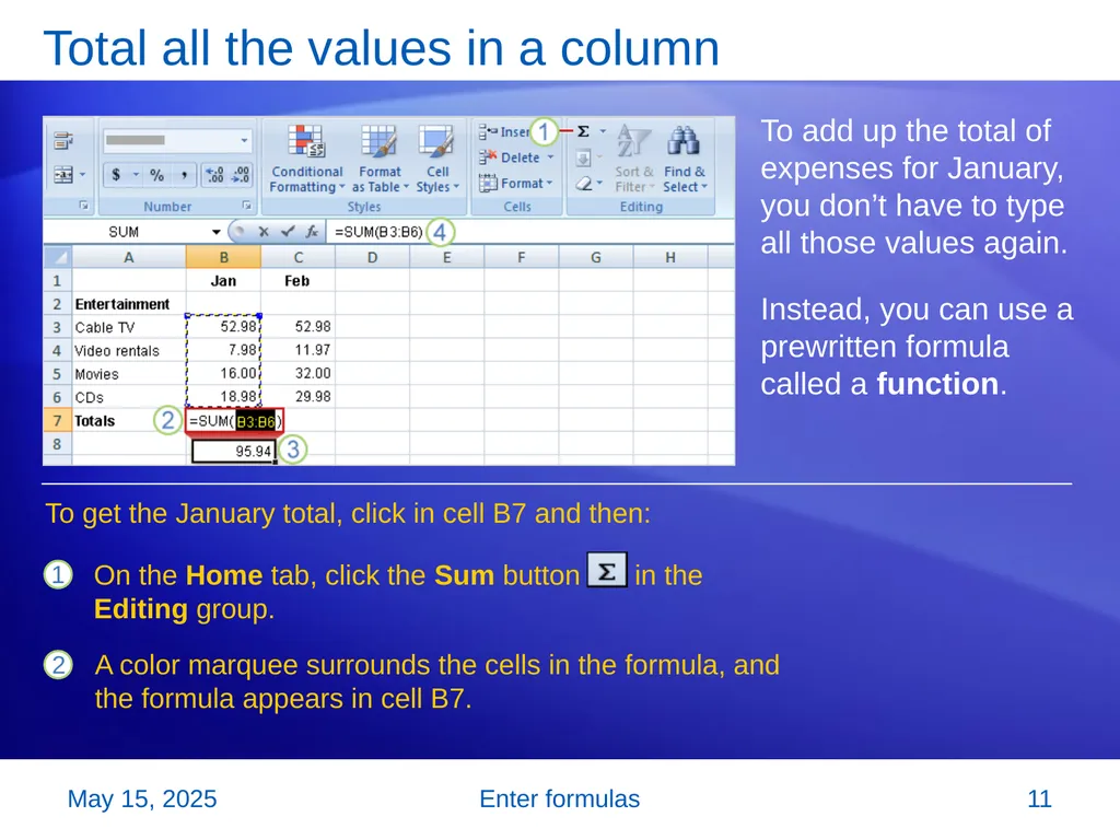
slide11. Enter formulas Total all the values in a column To add up the total of expenses for January, you don’t have to type all those values again.
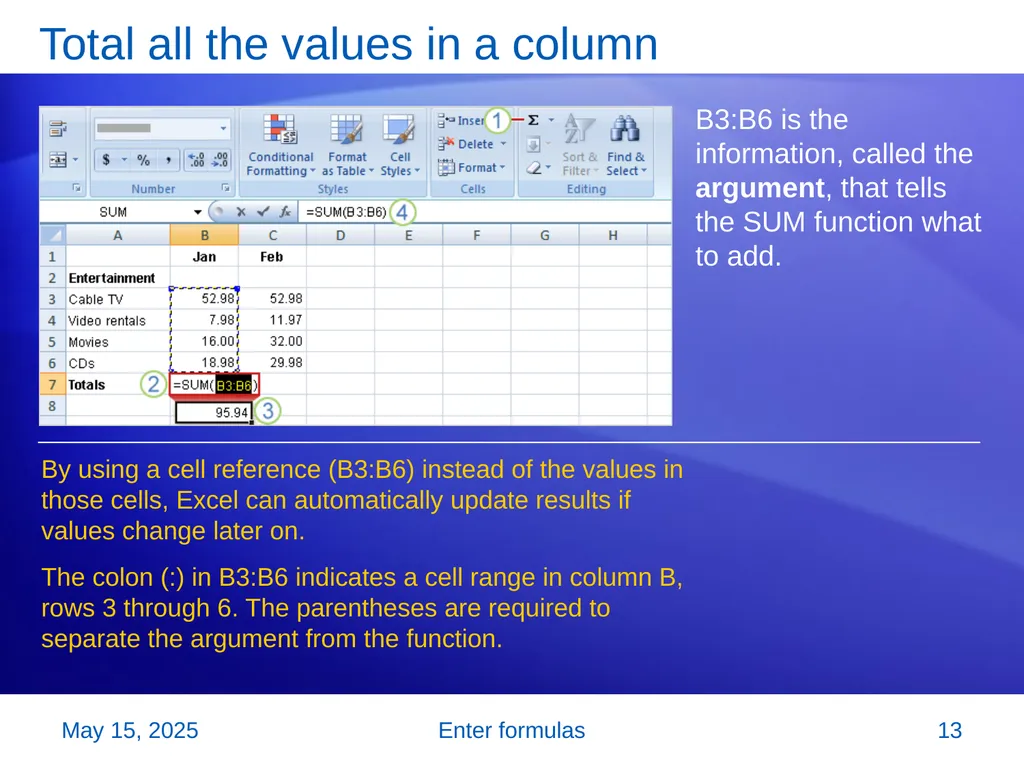
Instead, you can use a prewritten formula called a function. On the Home tab, click the Sum button in the Editing group. To get the January total, click in cell B7 and then: A color marquee surrounds the cells in the formula, and the formula appears in cell B7. 2 November 2007 11<br>
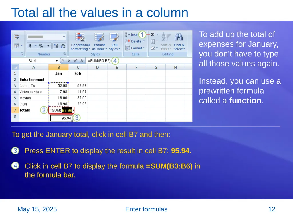
slide12. Enter formulas Total all the values in a column To add up the total of expenses for January, you don’t have to type all those values again.
Instead, you can use a prewritten formula called a function. Press ENTER to display the result in cell B7: 95.94. To get the January total, click in cell B7 and then: Click in cell B7 to display the formula =SUM(B3:B6) in the formula bar. 2 November 2007 12<br>
slide13. Enter formulas Total all the values in a column B3:B6 is the information, called the argument, that tells the SUM function what to add. By using a cell reference (B3:B6) instead of the values in those cells, Excel can automatically update results if values change later on.
The colon (:) in B3:B6 indicates a cell range in column B, rows 3 through 6. The parentheses are required to separate the argument from the function. 2 November 2007 13<br>
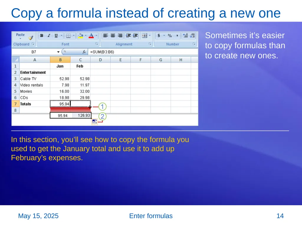
slide14. Enter formulas Copy a formula instead of creating a new one Sometimes it’s easier to copy formulas than to create new ones. In this section, you’ll see how to copy the formula you used to get the January total and use it to add up February’s expenses. 2 November 2007 14<br>
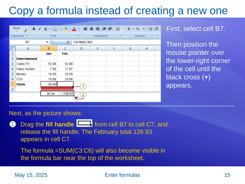
slide15. Enter formulas Copy a formula instead of creating a new one First, select cell B7. Next, as the picture shows: Then position the mouse pointer over the lower-right corner of the cell until the black cross (+) appears. Drag the fill handle from cell B7 to cell C7, and release the fill handle. The February total 126.93 appears in cell C7. The formula =SUM(C3:C6) will also become visible in the formula bar near the top of the worksheet. 2 November 2007 15<br>
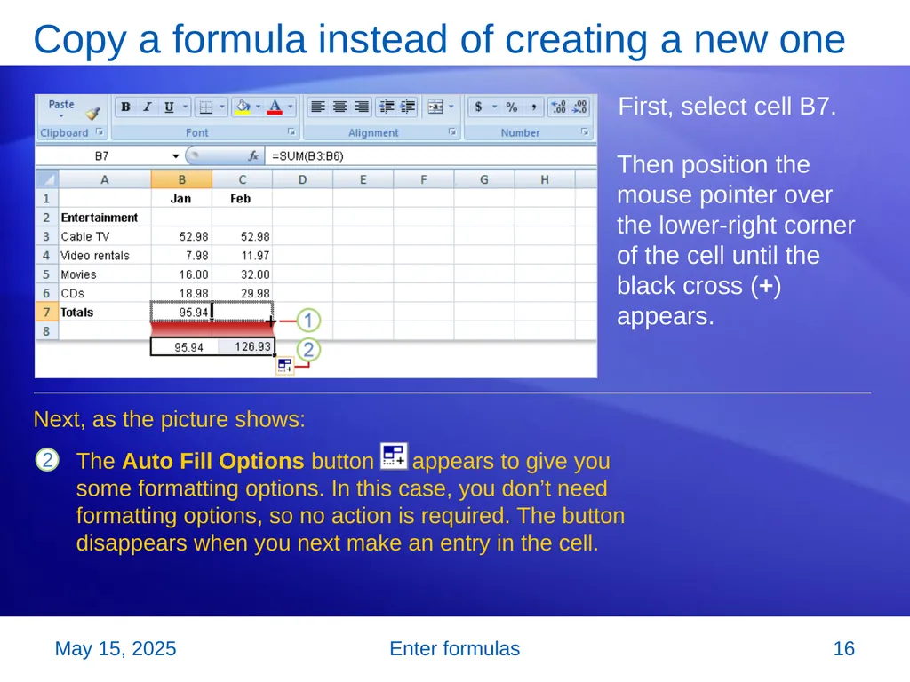
slide16. Enter formulas Copy a formula instead of creating a new one First, select cell B7. Next, as the picture shows: Then position the mouse pointer over the lower-right corner of the cell until the black cross (+) appears. The Auto Fill Options button appears to give you some formatting options. In this case, you don’t need formatting options, so no action is required. The button disappears when you next make an entry in the cell. 2 November 2007 16<br>
slide17. Enter formulas Suggestions for practice Create a formula for addition.
Create other formulas.
Add up a column of numbers.
Add up a row of numbers. Online practice (requires Excel 2007) 2 November 2007 17<br>
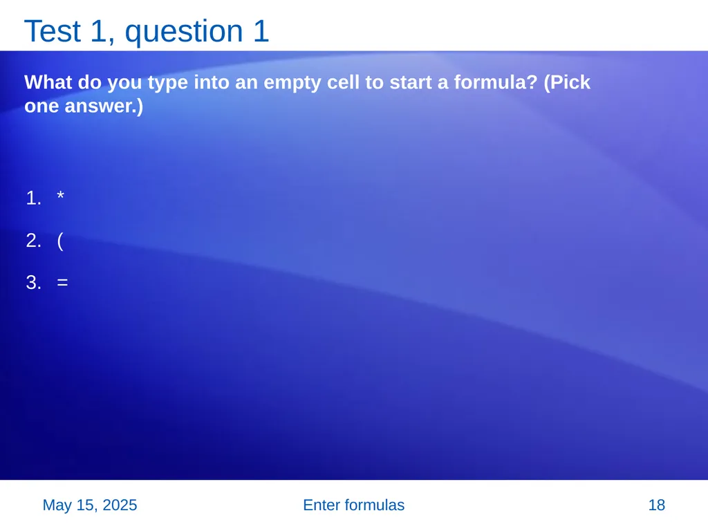
slide18. Enter formulas Test 1, question 1 What do you type into an empty cell to start a formula? (Pick one answer.) *
(
= 2 November 2007 18<br>
slide19. Enter formulas Test 1, question 1: Answer = An equal sign (=) tells Excel that a calculation follows it. 2 November 2007 19<br>
slide20. Enter formulas Test 1, question 2 What is a function? (Pick one answer.) A prewritten formula.
A math operator. 2 November 2007 20<br>
slide21. Enter formulas Test 1, question 2: Answer A prewritten formula. Functions are prewritten formulas, such as SUM, that save time. 2 November 2007 21<br>
slide22. Enter formulas Test 1, question 3 A formula result is in cell C6. You wonder how you got the result. To see the formula, what do you do? (Pick one answer.) Click in cell C6, and then press CTRL+SHIFT.
Click in cell C6, and then press F5.
Click in cell C6. 2 November 2007 22<br>
slide23. Enter formulas Test 1, question 3: Answer Click in cell C6. It’s that simple. The formula is visible in the formula bar near the top of the worksheet whenever you click in cell C6. Or you can double-click cell C6 to see the formula in cell C6. Then press ENTER to see the formula result again in the cell. 2 November 2007 23<br>
slide24. Lesson 2 Use cell references<br>
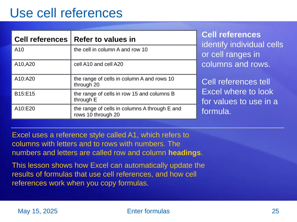
slide25. Enter formulas Use cell references Cell references identify individual cells or cell ranges in columns and rows.
Cell references tell Excel where to look for values to use in a formula. Excel uses a reference style called A1, which refers to columns with letters and to rows with numbers. The numbers and letters are called row and column headings.
This lesson shows how Excel can automatically update the results of formulas that use cell references, and how cell references work when you copy formulas. 2 November 2007 25<br>
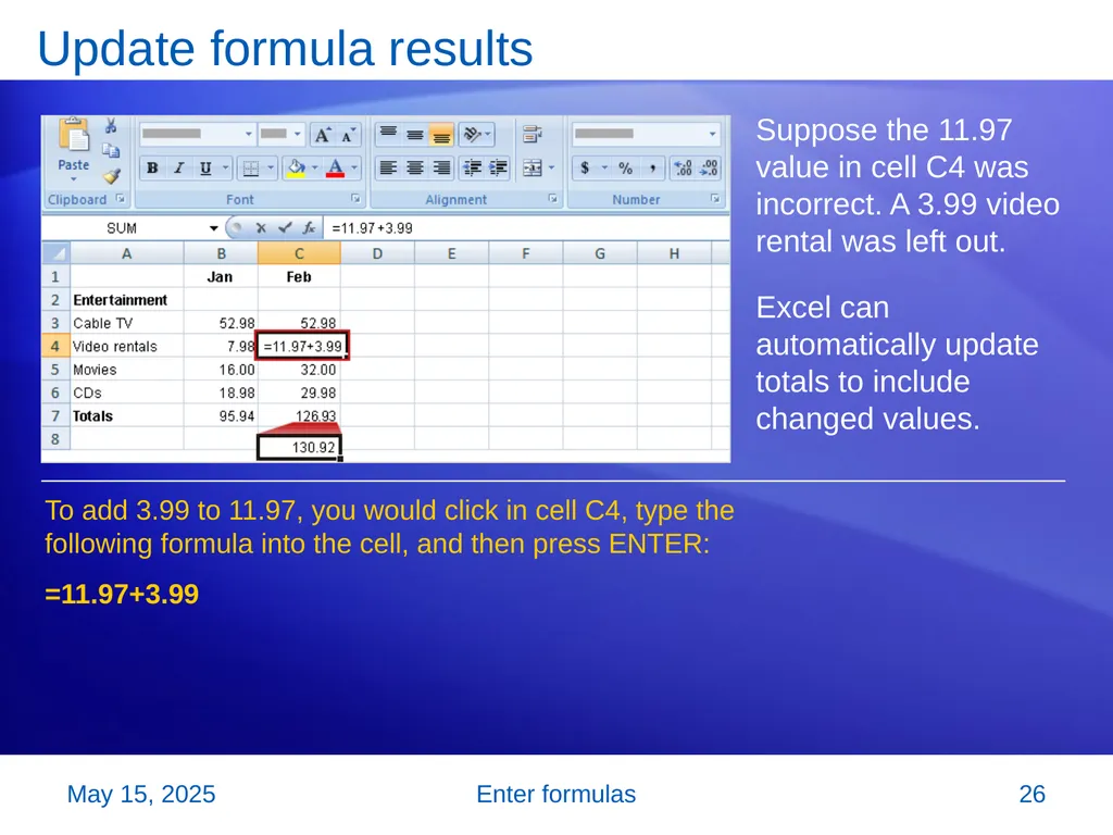
slide26. Enter formulas Update formula results Suppose the 11.97 value in cell C4 was incorrect. A 3.99 video rental was left out.
Excel can automatically update totals to include changed values. To add 3.99 to 11.97, you would click in cell C4, type the following formula into the cell, and then press ENTER:
=11.97+3.99 2 November 2007 26<br>
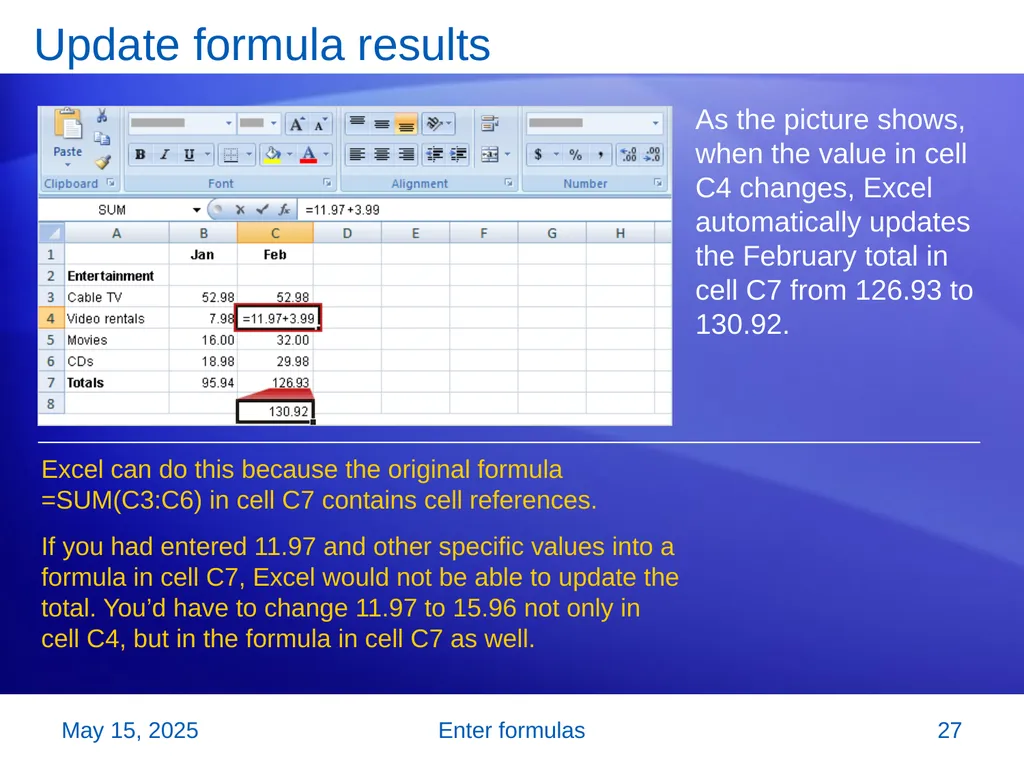
slide27. Enter formulas Update formula results As the picture shows, when the value in cell C4 changes, Excel automatically updates the February total in cell C7 from 126.93 to 130.92. Excel can do this because the original formula =SUM(C3:C6) in cell C7 contains cell references.
If you had entered 11.97 and other specific values into a formula in cell C7, Excel would not be able to update the total. You’d have to change 11.97 to 15.96 not only in cell C4, but in the formula in cell C7 as well. 2 November 2007 27<br>
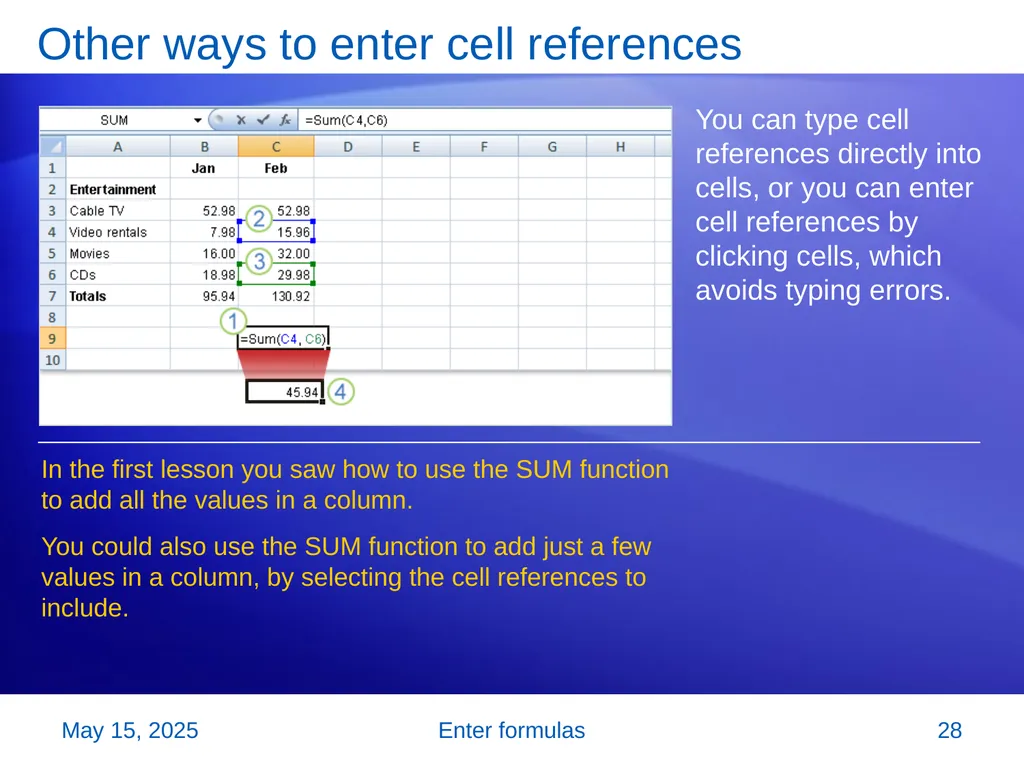
slide28. Enter formulas Other ways to enter cell references You can type cell references directly into cells, or you can enter cell references by clicking cells, which avoids typing errors. In the first lesson you saw how to use the SUM function to add all the values in a column.
You could also use the SUM function to add just a few values in a column, by selecting the cell references to include. 2 November 2007 28<br>
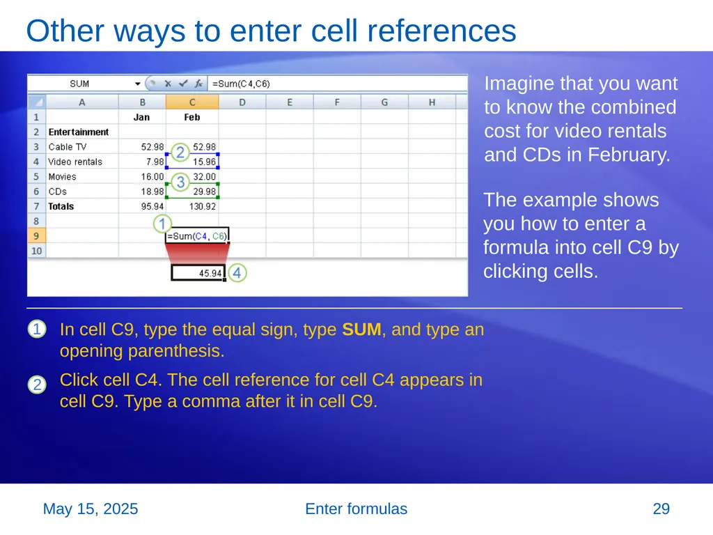
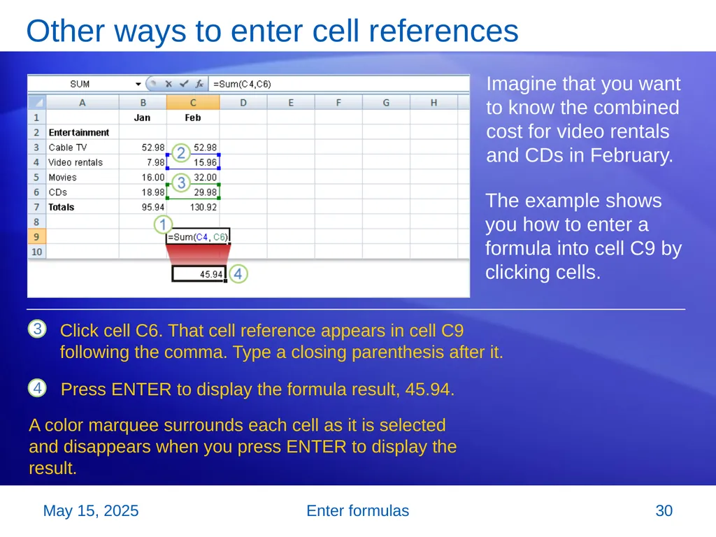
slide29. Enter formulas Other ways to enter cell references Imagine that you want to know the combined cost for video rentals and CDs in February. In cell C9, type the equal sign, type SUM, and type an opening parenthesis.
Click cell C4. The cell reference for cell C4 appears in cell C9. Type a comma after it in cell C9. The example shows you how to enter a formula into cell C9 by clicking cells. 2 November 2007 29<br>
slide30. Enter formulas Other ways to enter cell references Imagine that you want to know the combined cost for video rentals and CDs in February. Click cell C6. That cell reference appears in cell C9 following the comma. Type a closing parenthesis after it. The example shows you how to enter a formula into cell C9 by clicking cells. Press ENTER to display the formula result, 45.94. A color marquee surrounds each cell as it is selected and disappears when you press ENTER to display the result. 2 November 2007 30<br>
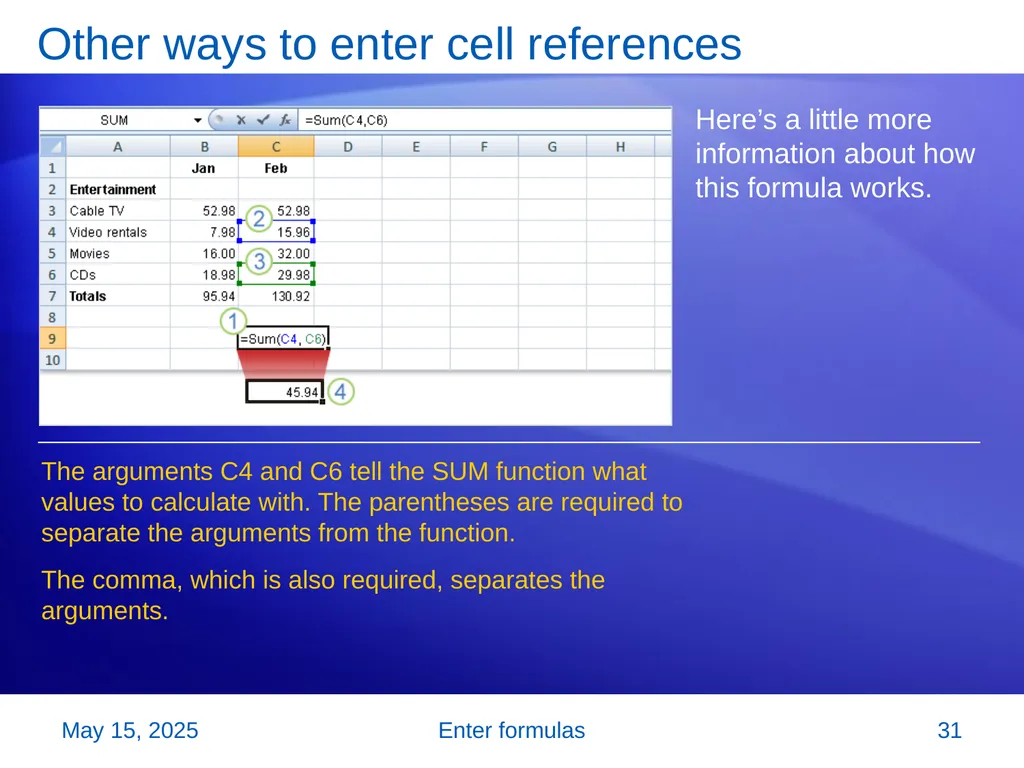
slide31. Enter formulas Other ways to enter cell references Here’s a little more information about how this formula works. The arguments C4 and C6 tell the SUM function what values to calculate with. The parentheses are required to separate the arguments from the function.
The comma, which is also required, separates the arguments. 2 November 2007 31<br>
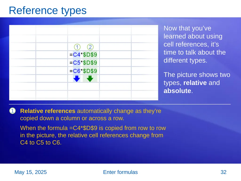
slide32. Enter formulas Reference types Now that you’ve learned about using cell references, it’s time to talk about the different types.
The picture shows two types, relative and absolute. Relative references automatically change as they’re copied down a column or across a row.
When the formula =C4*$D$9 is copied from row to row in the picture, the relative cell references change from C4 to C5 to C6. 2 November 2007 32<br>
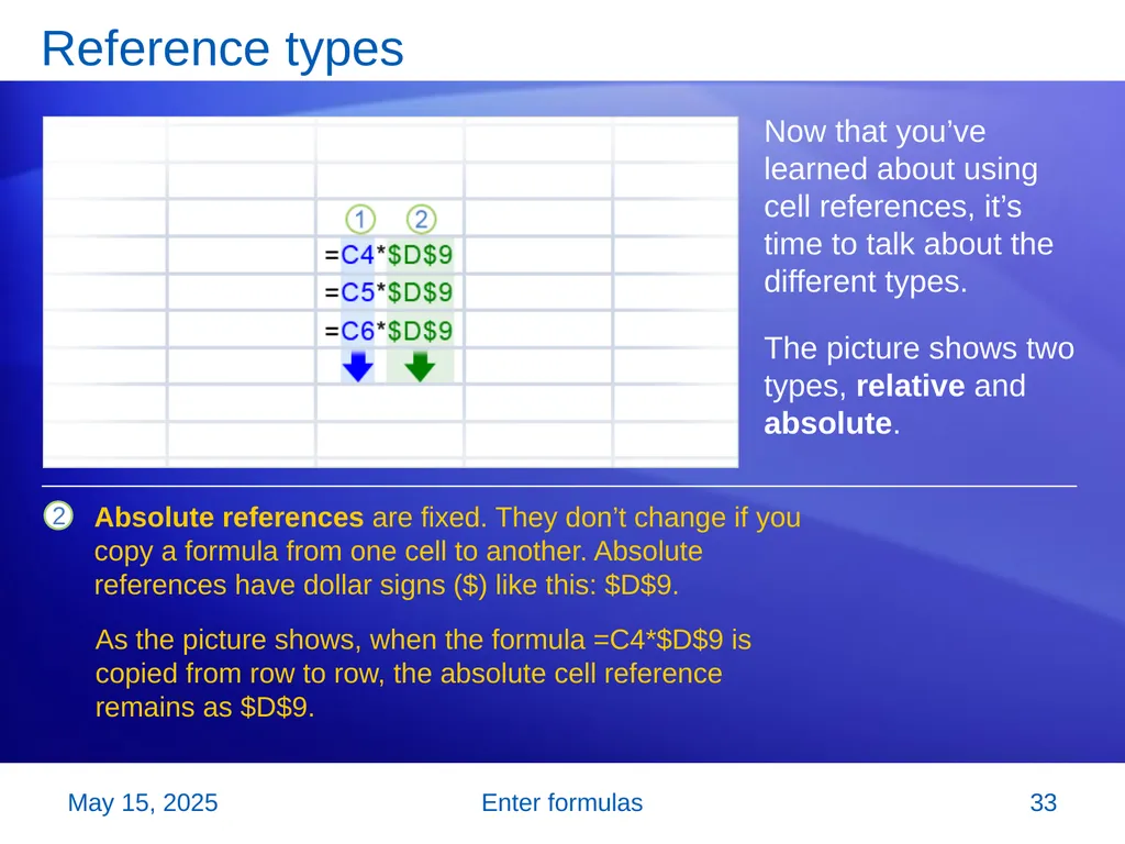
slide33. Enter formulas Reference types Now that you’ve learned about using cell references, it’s time to talk about the different types.
The picture shows two types, relative and absolute. Absolute references are fixed. They don’t change if you copy a formula from one cell to another. Absolute references have dollar signs ($) like this: $D$9. As the picture shows, when the formula =C4*$D$9 is copied from row to row, the absolute cell reference remains as $D$9. 2 November 2007 33<br>
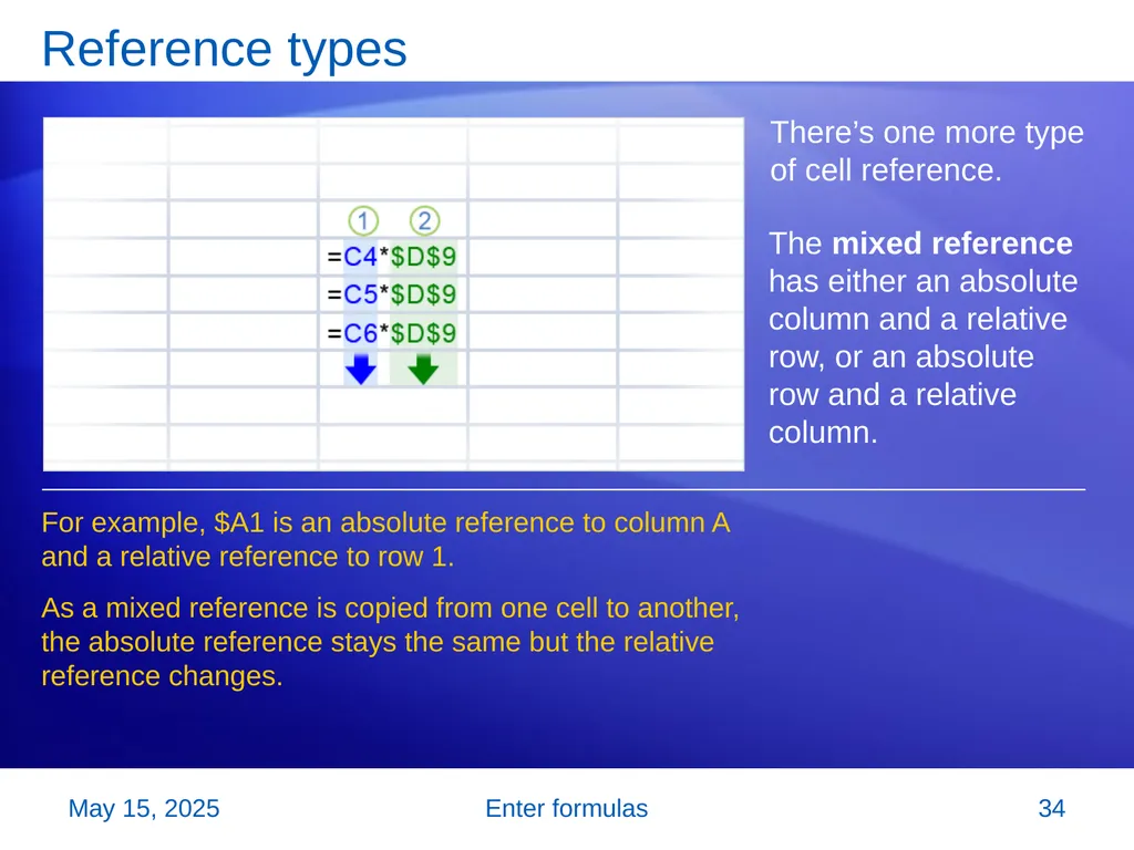
slide34. Enter formulas Reference types There’s one more type of cell reference. For example, $A1 is an absolute reference to column A and a relative reference to row 1.
As a mixed reference is copied from one cell to another, the absolute reference stays the same but the relative reference changes. The mixed reference has either an absolute column and a relative row, or an absolute row and a relative column. 2 November 2007 34<br>
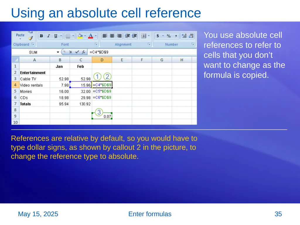
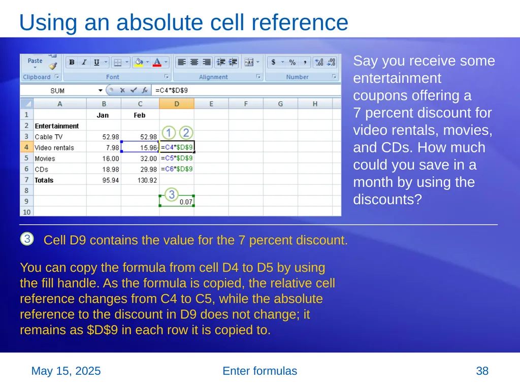
slide35. Enter formulas Using an absolute cell reference You use absolute cell references to refer to cells that you don’t want to change as the formula is copied. References are relative by default, so you would have to type dollar signs, as shown by callout 2 in the picture, to change the reference type to absolute. 2 November 2007 35<br>
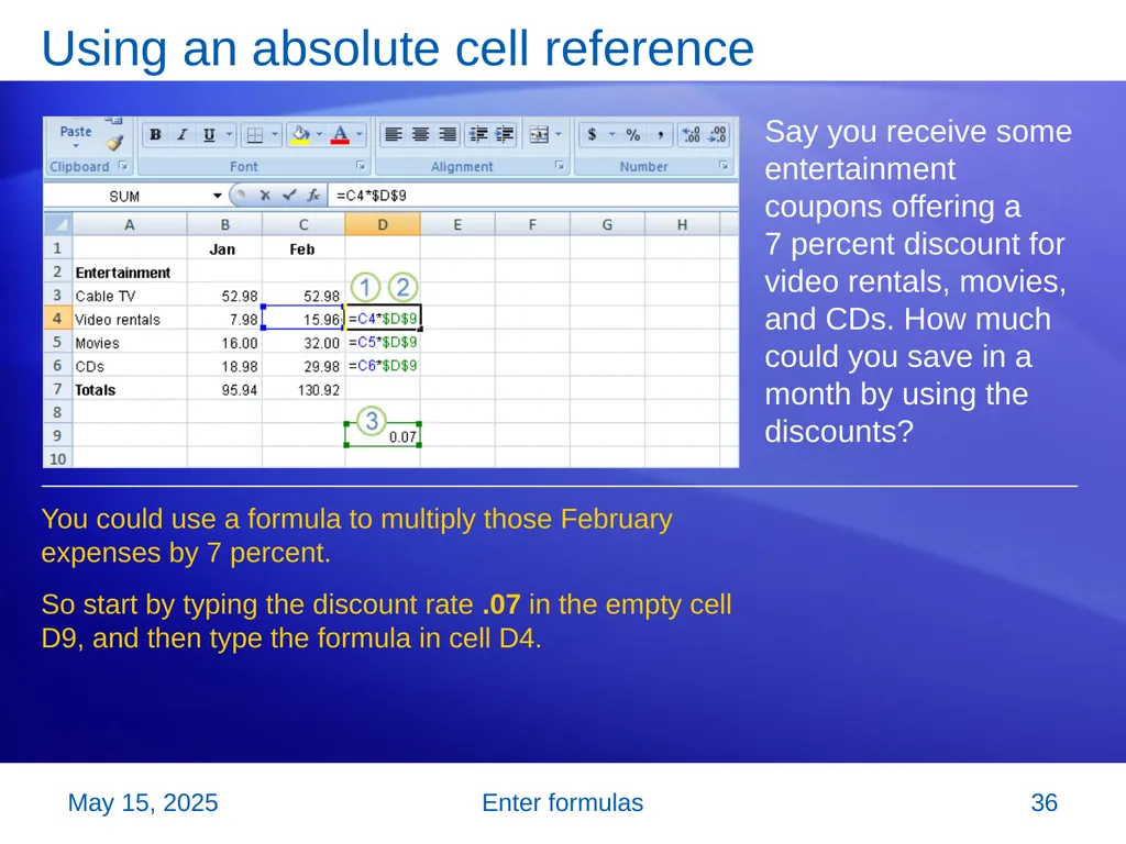
slide36. Enter formulas Using an absolute cell reference Say you receive some entertainment coupons offering a 7 percent discount for video rentals, movies, and CDs. How much could you save in a month by using the discounts? You could use a formula to multiply those February expenses by 7 percent.
So start by typing the discount rate .07 in the empty cell D9, and then type the formula in cell D4. 2 November 2007 36<br>
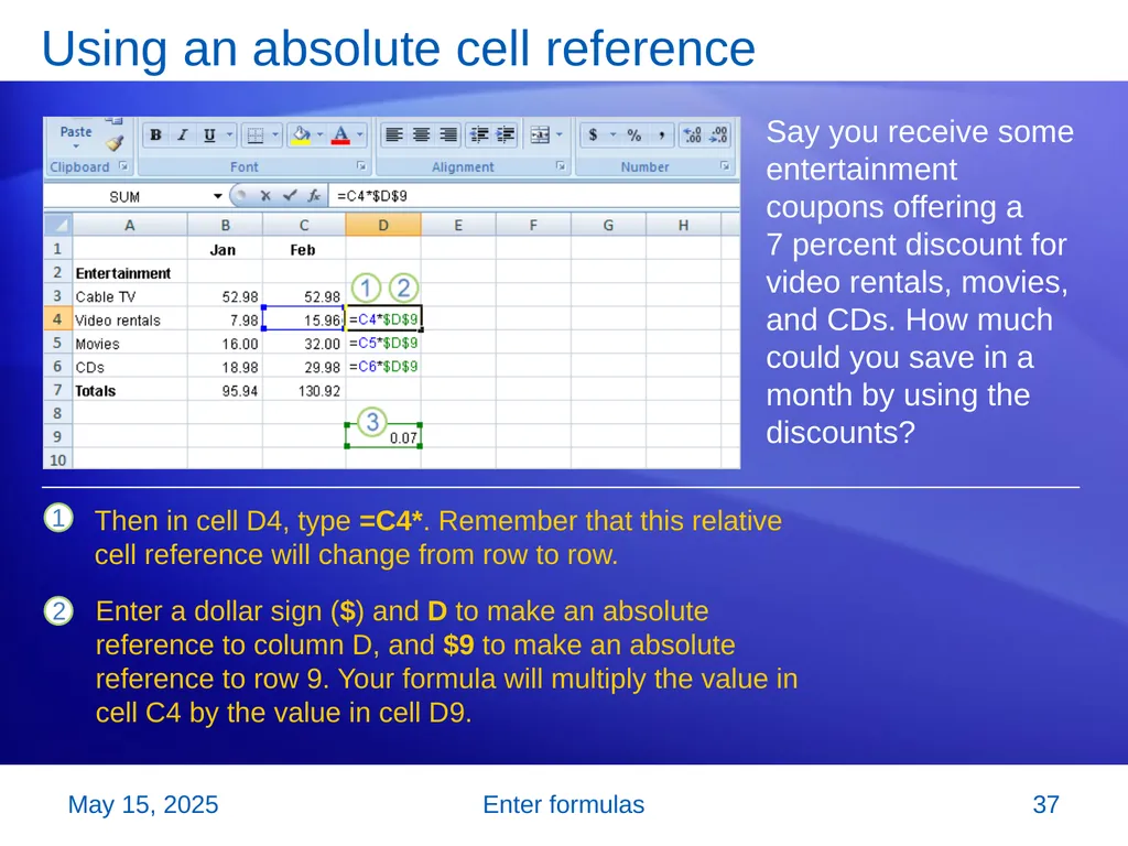
slide37. Enter formulas Using an absolute cell reference Say you receive some entertainment coupons offering a 7 percent discount for video rentals, movies, and CDs. How much could you save in a month by using the discounts? Then in cell D4, type =C4*. Remember that this relative cell reference will change from row to row. Enter a dollar sign ($) and D to make an absolute reference to column D, and $9 to make an absolute reference to row 9. Your formula will multiply the value in cell C4 by the value in cell D9. 2 November 2007 37<br>
slide38. Enter formulas Using an absolute cell reference Say you receive some entertainment coupons offering a 7 percent discount for video rentals, movies, and CDs. How much could you save in a month by using the discounts? Cell D9 contains the value for the 7 percent discount. You can copy the formula from cell D4 to D5 by using the fill handle. As the formula is copied, the relative cell reference changes from C4 to C5, while the absolute reference to the discount in D9 does not change; it remains as $D$9 in each row it is copied to. 2 November 2007 38<br>
slide39. Enter formulas Suggestions for practice Type cell references in a formula.
Select cell references for a formula.
Use an absolute reference in a formula.
Add up several results.
Change values and totals. Online practice (requires Excel 2007) 2 November 2007 39<br>
slide40. Enter formulas Test 2, question 1 How does an absolute cell reference work? (Pick one answer.) The cell reference automatically changes when the formula is copied down a column or across a row.
The cell reference is fixed.
The cell reference uses the A1 reference style. 2 November 2007 40<br>
slide41. Enter formulas Test 2, question 1: Answer The cell reference is fixed. Absolute cell references don’t change if you copy a formula from one cell to another. 2 November 2007 41<br>
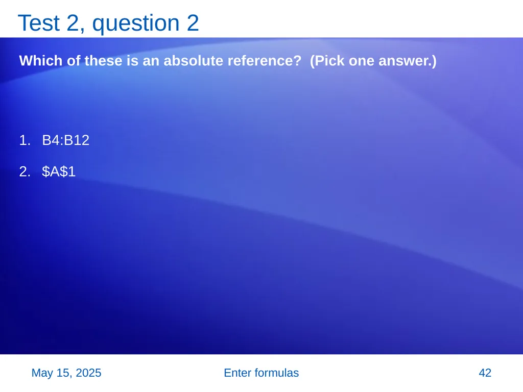
slide42. Enter formulas Test 2, question 2 Which of these is an absolute reference? (Pick one answer.) B4:B12
$A$1 2 November 2007 42<br>
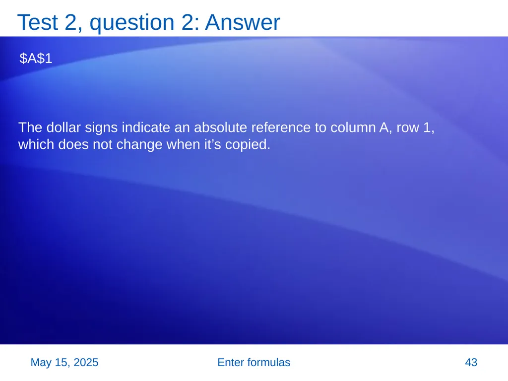
slide43. Enter formulas Test 2, question 2: Answer $A$1 The dollar signs indicate an absolute reference to column A, row 1, which does not change when it’s copied. 2 November 2007 43<br>
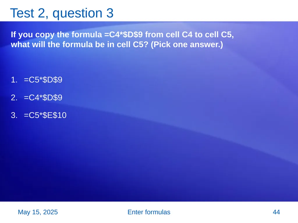
slide44. Enter formulas Test 2, question 3 If you copy the formula =C4*$D$9 from cell C4 to cell C5, what will the formula be in cell C5? (Pick one answer.) =C5*$D$9
=C4*$D$9
=C5*$E$10 2 November 2007 44<br>
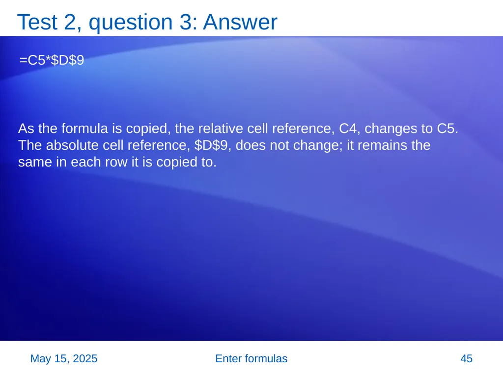
slide45. Enter formulas Test 2, question 3: Answer =C5*$D$9 As the formula is copied, the relative cell reference, C4, changes to C5. The absolute cell reference, $D$9, does not change; it remains the same in each row it is copied to. 2 November 2007 45<br>
slide46. Lesson 3 Simplify formulas by using functions<br>
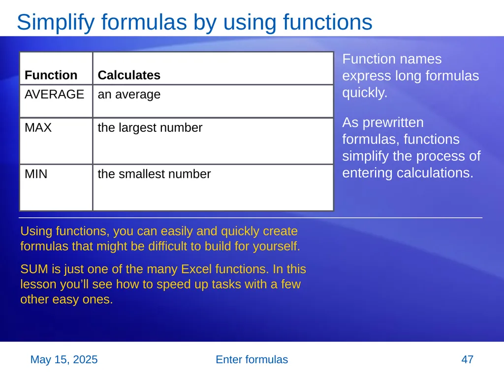
slide47. Enter formulas Simplify formulas by using functions Function names express long formulas quickly.
As prewritten formulas, functions simplify the process of entering calculations. Using functions, you can easily and quickly create formulas that might be difficult to build for yourself.
SUM is just one of the many Excel functions. In this lesson you’ll see how to speed up tasks with a few other easy ones. 2 November 2007 47<br>
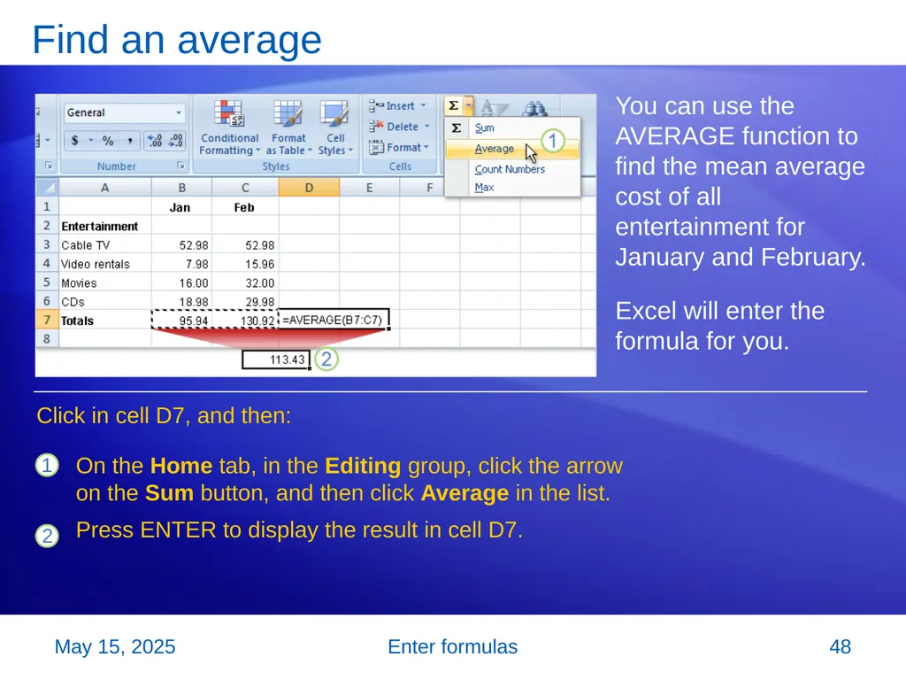
slide48. Enter formulas Find an average You can use the AVERAGE function to find the mean average cost of all entertainment for January and February.
Excel will enter the formula for you. Click in cell D7, and then: On the Home tab, in the Editing group, click the arrow on the Sum button, and then click Average in the list.
Press ENTER to display the result in cell D7. 2 November 2007 48<br>
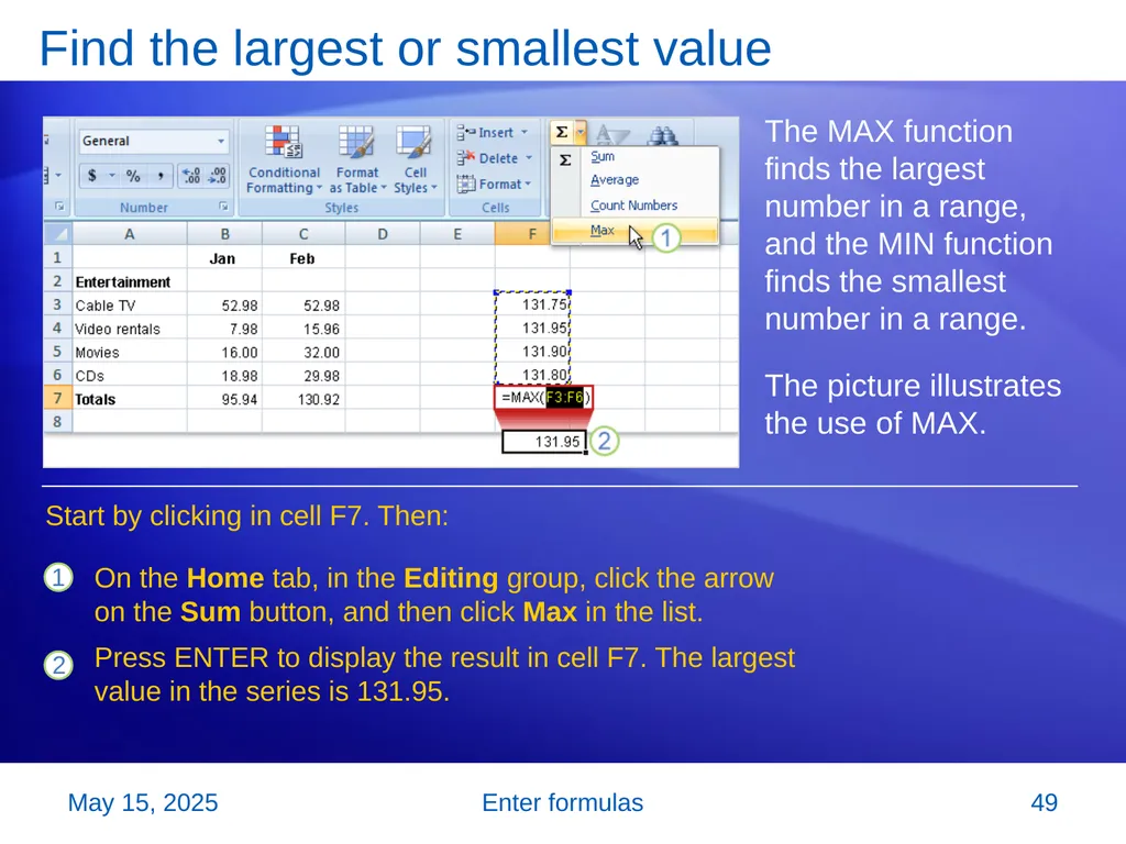
slide49. Enter formulas Find the largest or smallest value The MAX function finds the largest number in a range, and the MIN function finds the smallest number in a range.
The picture illustrates the use of MAX. Start by clicking in cell F7. Then: On the Home tab, in the Editing group, click the arrow on the Sum button, and then click Max in the list.
Press ENTER to display the result in cell F7. The largest value in the series is 131.95. 2 November 2007 49<br>
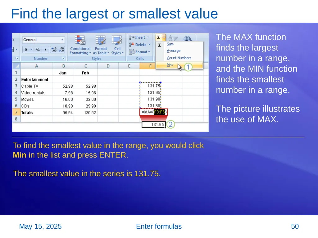
slide50. Enter formulas Find the largest or smallest value The MAX function finds the largest number in a range, and the MIN function finds the smallest number in a range.
The picture illustrates the use of MAX. To find the smallest value in the range, you would click Min in the list and press ENTER. The smallest value in the series is 131.75. 2 November 2007 50<br>
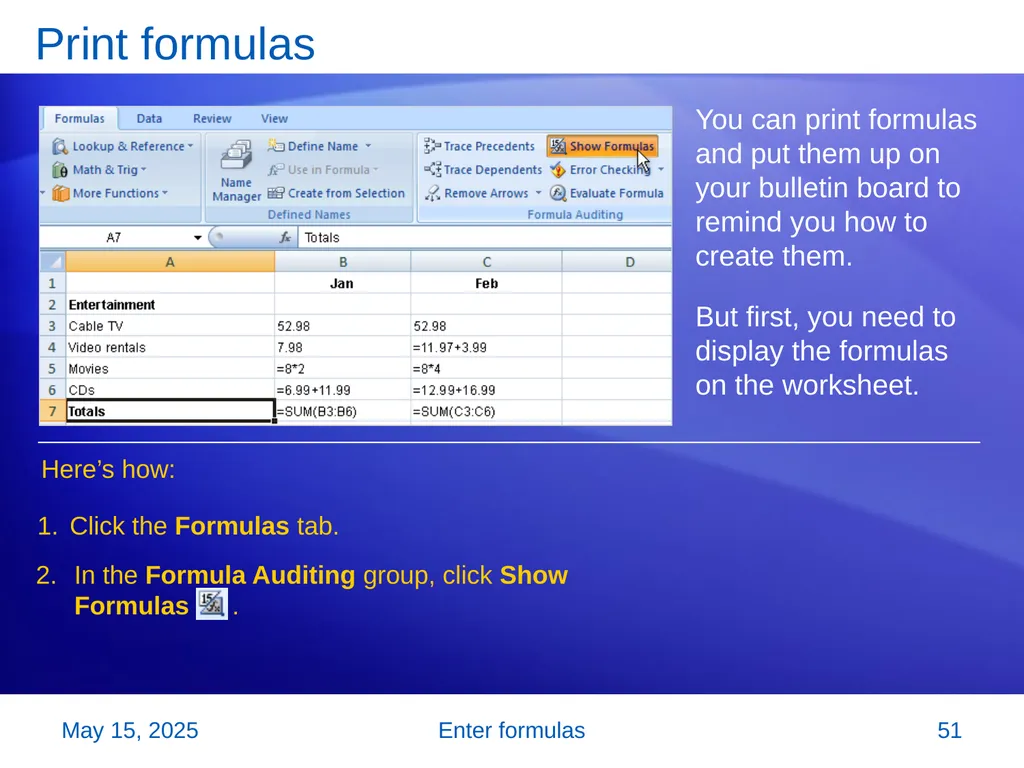
slide51. Enter formulas Print formulas You can print formulas and put them up on your bulletin board to remind you how to create them.
But first, you need to display the formulas on the worksheet. Here’s how: Click the Formulas tab. In the Formula Auditing group, click Show Formulas . 2 November 2007 51<br>
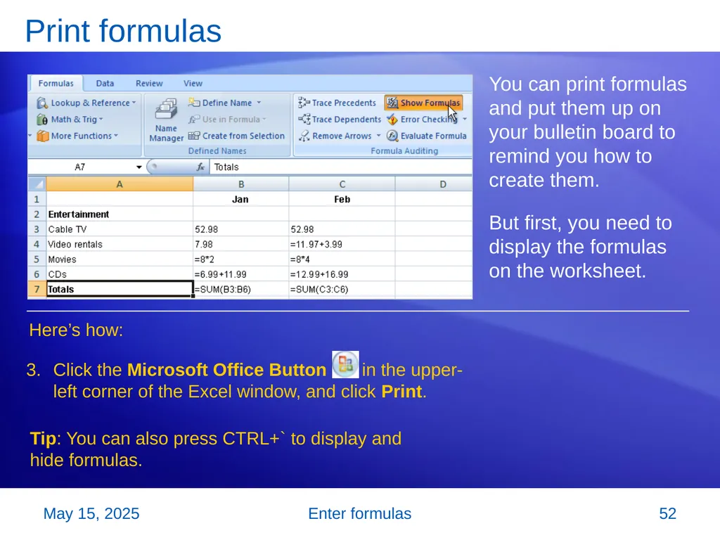
slide52. Enter formulas Print formulas You can print formulas and put them up on your bulletin board to remind you how to create them.
But first, you need to display the formulas on the worksheet. Here’s how: Click the Microsoft Office Button in the upper-left corner of the Excel window, and click Print. Tip: You can also press CTRL+` to display and hide formulas. 2 November 2007 52<br>
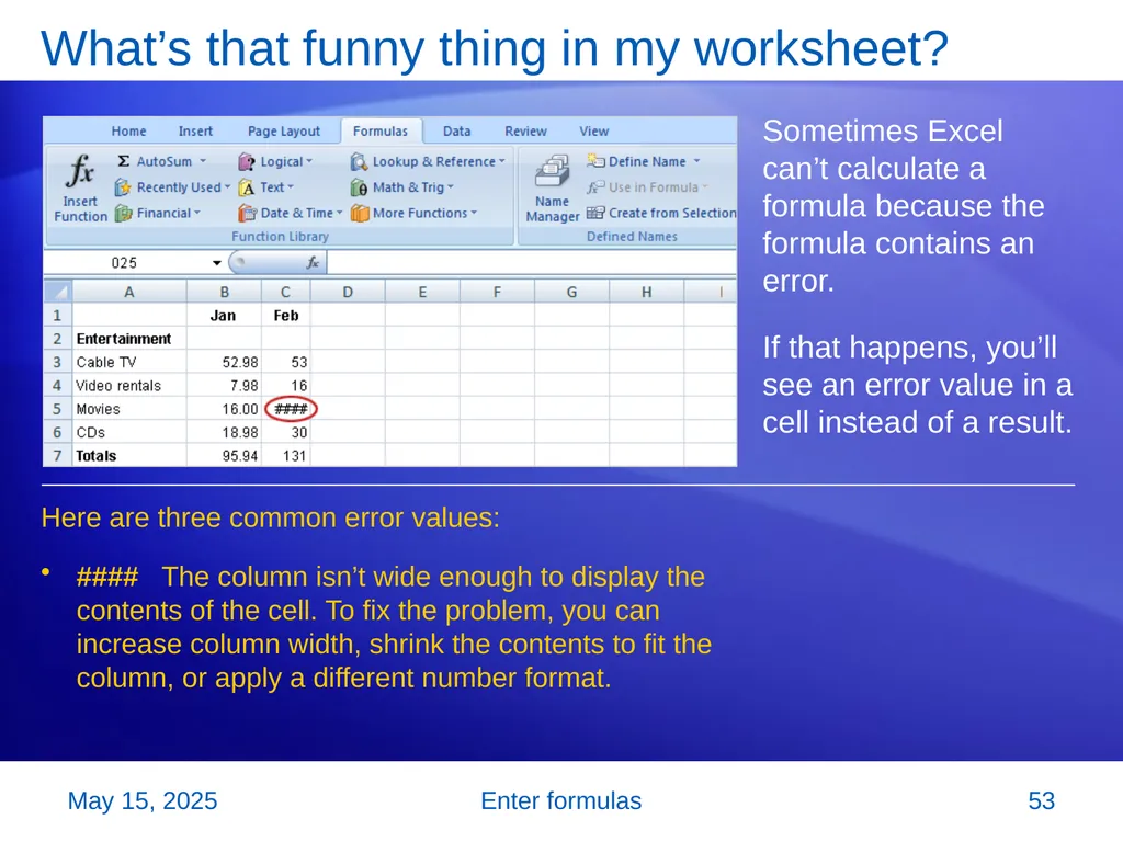
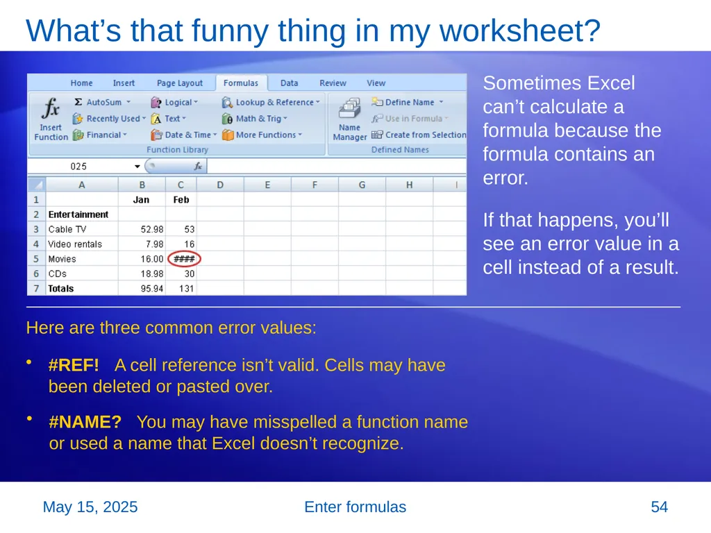
slide53. Enter formulas What’s that funny thing in my worksheet? Sometimes Excel can’t calculate a formula because the formula contains an error.
If that happens, you’ll see an error value in a cell instead of a result. #### The column isn’t wide enough to display the contents of the cell. To fix the problem, you can increase column width, shrink the contents to fit the column, or apply a different number format. Here are three common error values: 2 November 2007 53<br>
slide54. Enter formulas What’s that funny thing in my worksheet? Sometimes Excel can’t calculate a formula because the formula contains an error.
If that happens, you’ll see an error value in a cell instead of a result. #REF! A cell reference isn’t valid. Cells may have been deleted or pasted over. Here are three common error values: #NAME? You may have misspelled a function name or used a name that Excel doesn’t recognize. 2 November 2007 54<br>
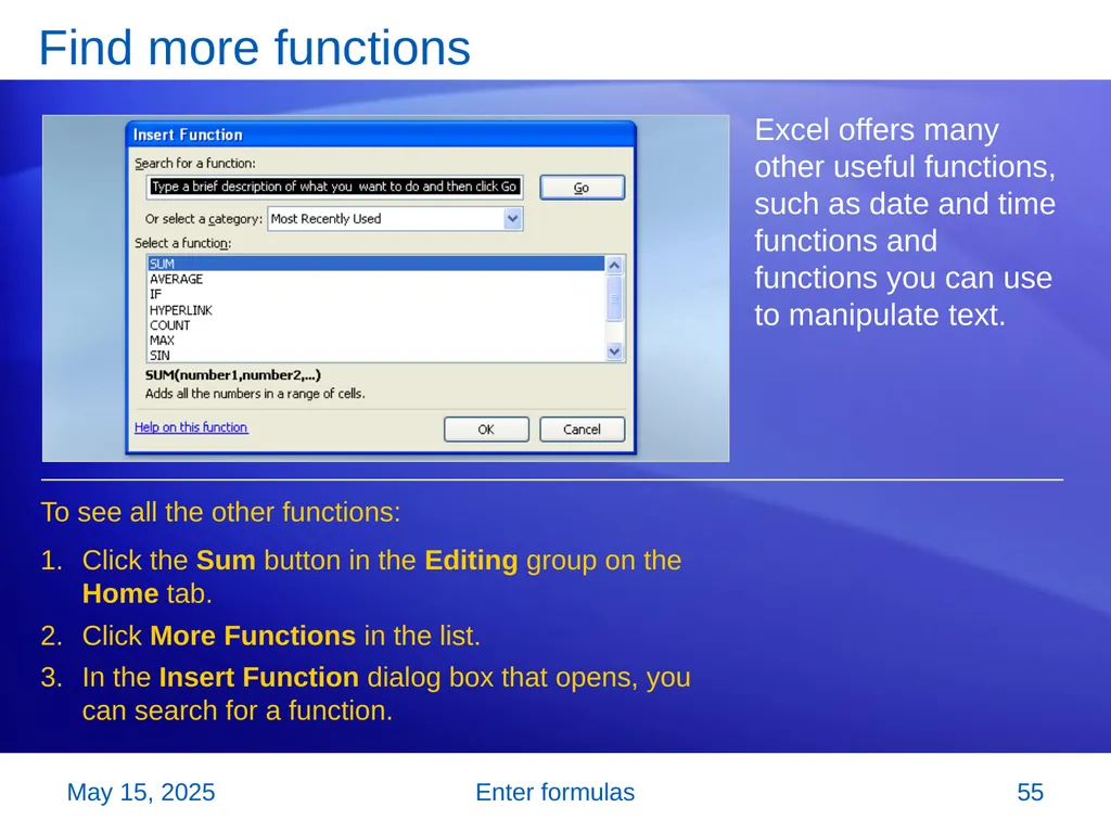
slide55. Enter formulas Find more functions Excel offers many other useful functions, such as date and time functions and functions you can use to manipulate text. Click the Sum button in the Editing group on the Home tab.
Click More Functions in the list.
In the Insert Function dialog box that opens, you can search for a function. To see all the other functions: 2 November 2007 55<br>
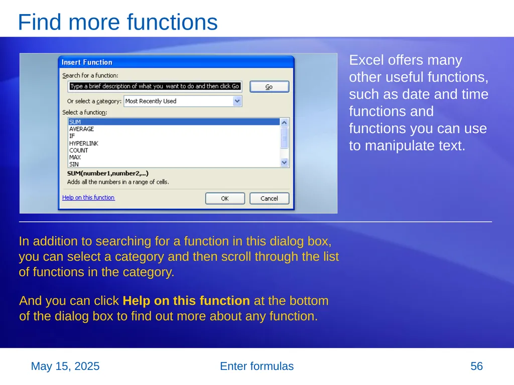
slide56. Enter formulas Find more functions Excel offers many other useful functions, such as date and time functions and functions you can use to manipulate text. In addition to searching for a function in this dialog box, you can select a category and then scroll through the list of functions in the category. And you can click Help on this function at the bottom of the dialog box to find out more about any function. 2 November 2007 56<br>
slide57. Enter formulas Suggestions for practice Find an average.
Find the largest number.
Find the smallest number.
Display and hide formulas.
Create and fix error values.
Create and fix the error value #NAME?. Online practice (requires Excel 2007) 2 November 2007 57<br>
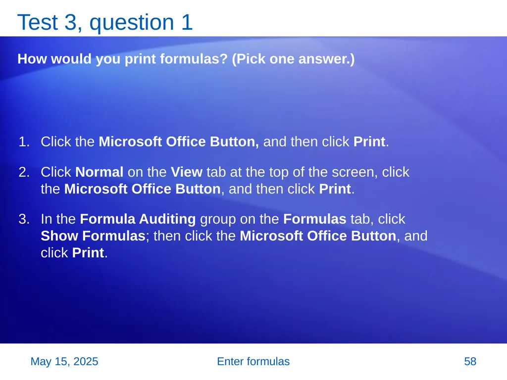
slide58. Enter formulas Test 3, question 1 How would you print formulas? (Pick one answer.) Click the Microsoft Office Button, and then click Print.
Click Normal on the View tab at the top of the screen, click the Microsoft Office Button, and then click Print.
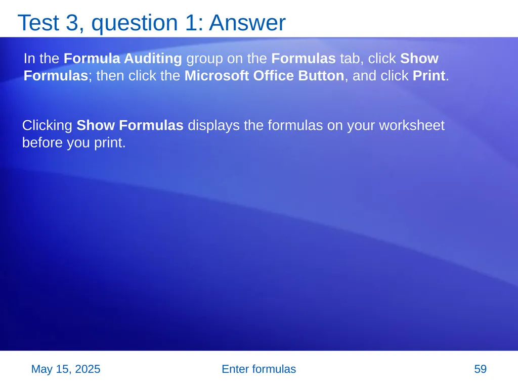
In the Formula Auditing group on the Formulas tab, click Show Formulas; then click the Microsoft Office Button, and click Print. 2 November 2007 58<br>
slide59. Enter formulas Test 3, question 1: Answer In the Formula Auditing group on the Formulas tab, click Show Formulas; then click the Microsoft Office Button, and click Print. Clicking Show Formulas displays the formulas on your worksheet before you print. 2 November 2007 59<br>
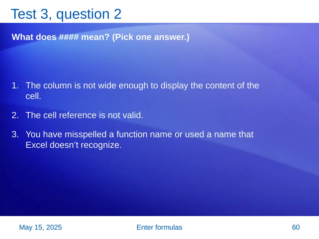
slide60. Enter formulas Test 3, question 2 What does #### mean? (Pick one answer.) The column is not wide enough to display the content of the cell.
The cell reference is not valid.
You have misspelled a function name or used a name that Excel doesn’t recognize. 2 November 2007 60<br>
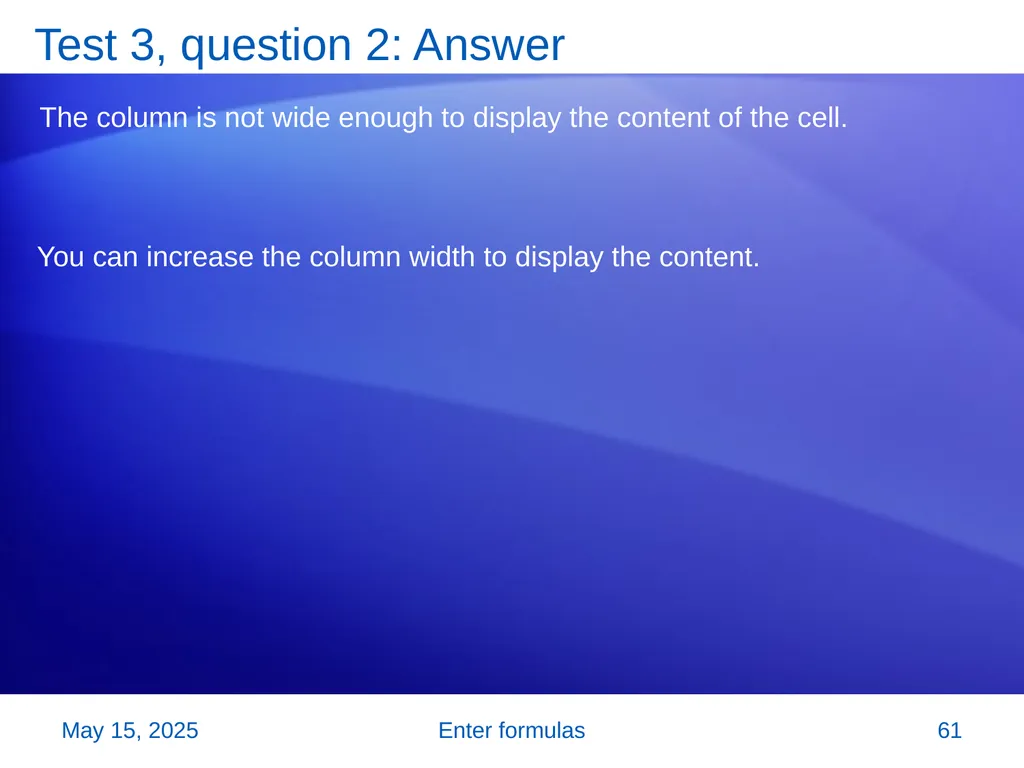
slide61. Enter formulas Test 3, question 2: Answer The column is not wide enough to display the content of the cell. You can increase the column width to display the content. 2 November 2007 61<br>
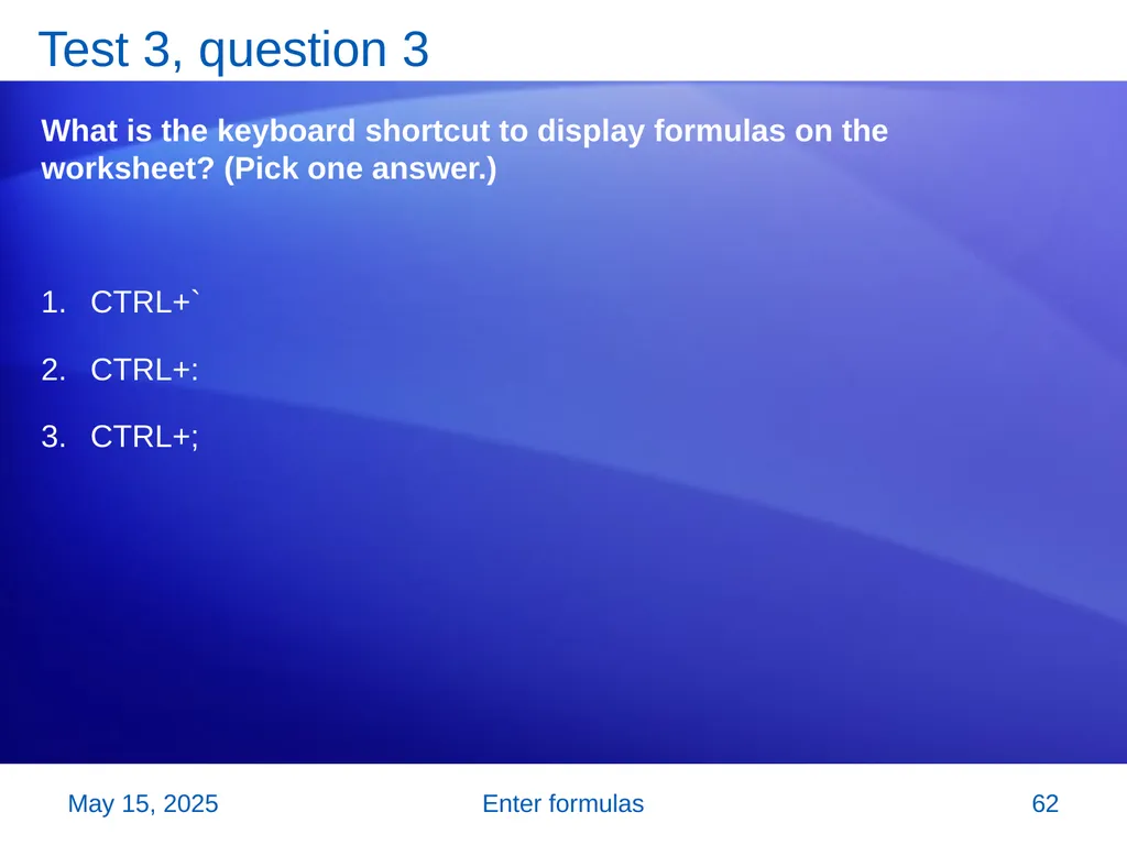
slide62. Enter formulas Test 3, question 3 What is the keyboard shortcut to display formulas on the worksheet? (Pick one answer.) CTRL+`
CTRL+:
CTRL+; 2 November 2007 62<br>
slide63. Enter formulas Test 3, question 3: Answer CTRL+` The ` is next to the 1 key on most keyboards. The keyboard shortcut displays and hides formulas. 2 November 2007 63<br>
slide64. Enter formulas Quick Reference Card For a summary of the tasks covered in this course, view the Quick Reference Card. 2 November 2007 64<br>
slide65. USING THIS TEMPLATE See the notes pane or view the full notes page (View tab) for detailed help on this template.<br>
slide2. Enter formulas Course contents Overview: Goodbye, calculator
Lesson 1: Get started
Lesson 2: Use cell references
Lesson 3: Simplify formulas by using functions Each lesson includes a list of suggested tasks and a set of test questions. 2 November 2007 2<br>
slide3. Enter formulas Overview: Goodbye, calculator Excel is great for working with numbers and math. In this course you’ll learn how add, divide, multiply, and subtract by typing formulas into Excel worksheets.
You’ll also learn how to use simple formulas that automatically update their results when values change.
After picking up the techniques in this course, you’ll be able to put your calculator away for good. 2 November 2007 3<br>
slide4. Enter formulas Course goals Do math by typing simple formulas to add, divide, multiply, and subtract.
Use cell references in formulas, so that Excel can automatically update results when values change or when you copy formulas.
Use functions (prewritten formulas) to add up values, calculate averages, and find the smallest or largest value in a range of values. 2 November 2007 4<br>
slide5. Lesson 1 Get started<br>
slide6. Enter formulas Get started Imagine that Excel is open and you’re looking at the “Entertainment” section of a household expense budget. Cell C6 in the worksheet is empty; the amount spent for CDs in February hasn’t been entered yet.
In this lesson, you’ll learn how to use Excel to do basic math by typing simple formulas into cells. You’ll also learn how to total all the values in a column with a formula that updates its result if values change later. 2 November 2007 6<br>
slide7. Enter formulas Begin with an equal sign The two CDs purchased in February cost $12.99 and $16.99. The total of these two values is the CD expense for the month.
You can add these values in Excel by typing a simple formula into cell C6. 2 November 2007 7<br>
slide8. Enter formulas Begin with an equal sign The picture illustrates what to do. Type a formula in cell C6. Excel formulas always begin with an equal sign. To add 12.99 and 16.99, type:
=12.99+16.99 The plus sign (+) is the math operator that tells Excel to add the values. 2 November 2007 8<br>
slide9. Enter formulas Begin with an equal sign The picture illustrates what to do. Press ENTER to display the formula result. If you wonder later how you got this result, you can click in cell C6 any time and view the formula in the formula bar near the top of the worksheet. 2 November 2007 9<br>
slide10. Enter formulas Use other math operators To do more than add, use other math operators as you type formulas into worksheet cells.
Excel uses familiar signs to build formulas. As the table shows, use a minus sign (-) to subtract, an asterisk (*) to multiply, and a forward slash (/) to divide.
Remember to always start each formula with an equal sign. 2 November 2007 10<br>
slide11. Enter formulas Total all the values in a column To add up the total of expenses for January, you don’t have to type all those values again.
Instead, you can use a prewritten formula called a function. On the Home tab, click the Sum button in the Editing group. To get the January total, click in cell B7 and then: A color marquee surrounds the cells in the formula, and the formula appears in cell B7. 2 November 2007 11<br>
slide12. Enter formulas Total all the values in a column To add up the total of expenses for January, you don’t have to type all those values again.
Instead, you can use a prewritten formula called a function. Press ENTER to display the result in cell B7: 95.94. To get the January total, click in cell B7 and then: Click in cell B7 to display the formula =SUM(B3:B6) in the formula bar. 2 November 2007 12<br>
slide13. Enter formulas Total all the values in a column B3:B6 is the information, called the argument, that tells the SUM function what to add. By using a cell reference (B3:B6) instead of the values in those cells, Excel can automatically update results if values change later on.
The colon (:) in B3:B6 indicates a cell range in column B, rows 3 through 6. The parentheses are required to separate the argument from the function. 2 November 2007 13<br>
slide14. Enter formulas Copy a formula instead of creating a new one Sometimes it’s easier to copy formulas than to create new ones. In this section, you’ll see how to copy the formula you used to get the January total and use it to add up February’s expenses. 2 November 2007 14<br>
slide15. Enter formulas Copy a formula instead of creating a new one First, select cell B7. Next, as the picture shows: Then position the mouse pointer over the lower-right corner of the cell until the black cross (+) appears. Drag the fill handle from cell B7 to cell C7, and release the fill handle. The February total 126.93 appears in cell C7. The formula =SUM(C3:C6) will also become visible in the formula bar near the top of the worksheet. 2 November 2007 15<br>
slide16. Enter formulas Copy a formula instead of creating a new one First, select cell B7. Next, as the picture shows: Then position the mouse pointer over the lower-right corner of the cell until the black cross (+) appears. The Auto Fill Options button appears to give you some formatting options. In this case, you don’t need formatting options, so no action is required. The button disappears when you next make an entry in the cell. 2 November 2007 16<br>
slide17. Enter formulas Suggestions for practice Create a formula for addition.
Create other formulas.
Add up a column of numbers.
Add up a row of numbers. Online practice (requires Excel 2007) 2 November 2007 17<br>
slide18. Enter formulas Test 1, question 1 What do you type into an empty cell to start a formula? (Pick one answer.) *
(
= 2 November 2007 18<br>
slide19. Enter formulas Test 1, question 1: Answer = An equal sign (=) tells Excel that a calculation follows it. 2 November 2007 19<br>
slide20. Enter formulas Test 1, question 2 What is a function? (Pick one answer.) A prewritten formula.
A math operator. 2 November 2007 20<br>
slide21. Enter formulas Test 1, question 2: Answer A prewritten formula. Functions are prewritten formulas, such as SUM, that save time. 2 November 2007 21<br>
slide22. Enter formulas Test 1, question 3 A formula result is in cell C6. You wonder how you got the result. To see the formula, what do you do? (Pick one answer.) Click in cell C6, and then press CTRL+SHIFT.
Click in cell C6, and then press F5.
Click in cell C6. 2 November 2007 22<br>
slide23. Enter formulas Test 1, question 3: Answer Click in cell C6. It’s that simple. The formula is visible in the formula bar near the top of the worksheet whenever you click in cell C6. Or you can double-click cell C6 to see the formula in cell C6. Then press ENTER to see the formula result again in the cell. 2 November 2007 23<br>
slide24. Lesson 2 Use cell references<br>
slide25. Enter formulas Use cell references Cell references identify individual cells or cell ranges in columns and rows.
Cell references tell Excel where to look for values to use in a formula. Excel uses a reference style called A1, which refers to columns with letters and to rows with numbers. The numbers and letters are called row and column headings.
This lesson shows how Excel can automatically update the results of formulas that use cell references, and how cell references work when you copy formulas. 2 November 2007 25<br>
slide26. Enter formulas Update formula results Suppose the 11.97 value in cell C4 was incorrect. A 3.99 video rental was left out.
Excel can automatically update totals to include changed values. To add 3.99 to 11.97, you would click in cell C4, type the following formula into the cell, and then press ENTER:
=11.97+3.99 2 November 2007 26<br>
slide27. Enter formulas Update formula results As the picture shows, when the value in cell C4 changes, Excel automatically updates the February total in cell C7 from 126.93 to 130.92. Excel can do this because the original formula =SUM(C3:C6) in cell C7 contains cell references.
If you had entered 11.97 and other specific values into a formula in cell C7, Excel would not be able to update the total. You’d have to change 11.97 to 15.96 not only in cell C4, but in the formula in cell C7 as well. 2 November 2007 27<br>
slide28. Enter formulas Other ways to enter cell references You can type cell references directly into cells, or you can enter cell references by clicking cells, which avoids typing errors. In the first lesson you saw how to use the SUM function to add all the values in a column.
You could also use the SUM function to add just a few values in a column, by selecting the cell references to include. 2 November 2007 28<br>
slide29. Enter formulas Other ways to enter cell references Imagine that you want to know the combined cost for video rentals and CDs in February. In cell C9, type the equal sign, type SUM, and type an opening parenthesis.
Click cell C4. The cell reference for cell C4 appears in cell C9. Type a comma after it in cell C9. The example shows you how to enter a formula into cell C9 by clicking cells. 2 November 2007 29<br>
slide30. Enter formulas Other ways to enter cell references Imagine that you want to know the combined cost for video rentals and CDs in February. Click cell C6. That cell reference appears in cell C9 following the comma. Type a closing parenthesis after it. The example shows you how to enter a formula into cell C9 by clicking cells. Press ENTER to display the formula result, 45.94. A color marquee surrounds each cell as it is selected and disappears when you press ENTER to display the result. 2 November 2007 30<br>
slide31. Enter formulas Other ways to enter cell references Here’s a little more information about how this formula works. The arguments C4 and C6 tell the SUM function what values to calculate with. The parentheses are required to separate the arguments from the function.
The comma, which is also required, separates the arguments. 2 November 2007 31<br>
slide32. Enter formulas Reference types Now that you’ve learned about using cell references, it’s time to talk about the different types.
The picture shows two types, relative and absolute. Relative references automatically change as they’re copied down a column or across a row.
When the formula =C4*$D$9 is copied from row to row in the picture, the relative cell references change from C4 to C5 to C6. 2 November 2007 32<br>
slide33. Enter formulas Reference types Now that you’ve learned about using cell references, it’s time to talk about the different types.
The picture shows two types, relative and absolute. Absolute references are fixed. They don’t change if you copy a formula from one cell to another. Absolute references have dollar signs ($) like this: $D$9. As the picture shows, when the formula =C4*$D$9 is copied from row to row, the absolute cell reference remains as $D$9. 2 November 2007 33<br>
slide34. Enter formulas Reference types There’s one more type of cell reference. For example, $A1 is an absolute reference to column A and a relative reference to row 1.
As a mixed reference is copied from one cell to another, the absolute reference stays the same but the relative reference changes. The mixed reference has either an absolute column and a relative row, or an absolute row and a relative column. 2 November 2007 34<br>
slide35. Enter formulas Using an absolute cell reference You use absolute cell references to refer to cells that you don’t want to change as the formula is copied. References are relative by default, so you would have to type dollar signs, as shown by callout 2 in the picture, to change the reference type to absolute. 2 November 2007 35<br>
slide36. Enter formulas Using an absolute cell reference Say you receive some entertainment coupons offering a 7 percent discount for video rentals, movies, and CDs. How much could you save in a month by using the discounts? You could use a formula to multiply those February expenses by 7 percent.
So start by typing the discount rate .07 in the empty cell D9, and then type the formula in cell D4. 2 November 2007 36<br>
slide37. Enter formulas Using an absolute cell reference Say you receive some entertainment coupons offering a 7 percent discount for video rentals, movies, and CDs. How much could you save in a month by using the discounts? Then in cell D4, type =C4*. Remember that this relative cell reference will change from row to row. Enter a dollar sign ($) and D to make an absolute reference to column D, and $9 to make an absolute reference to row 9. Your formula will multiply the value in cell C4 by the value in cell D9. 2 November 2007 37<br>
slide38. Enter formulas Using an absolute cell reference Say you receive some entertainment coupons offering a 7 percent discount for video rentals, movies, and CDs. How much could you save in a month by using the discounts? Cell D9 contains the value for the 7 percent discount. You can copy the formula from cell D4 to D5 by using the fill handle. As the formula is copied, the relative cell reference changes from C4 to C5, while the absolute reference to the discount in D9 does not change; it remains as $D$9 in each row it is copied to. 2 November 2007 38<br>
slide39. Enter formulas Suggestions for practice Type cell references in a formula.
Select cell references for a formula.
Use an absolute reference in a formula.
Add up several results.
Change values and totals. Online practice (requires Excel 2007) 2 November 2007 39<br>
slide40. Enter formulas Test 2, question 1 How does an absolute cell reference work? (Pick one answer.) The cell reference automatically changes when the formula is copied down a column or across a row.
The cell reference is fixed.
The cell reference uses the A1 reference style. 2 November 2007 40<br>
slide41. Enter formulas Test 2, question 1: Answer The cell reference is fixed. Absolute cell references don’t change if you copy a formula from one cell to another. 2 November 2007 41<br>
slide42. Enter formulas Test 2, question 2 Which of these is an absolute reference? (Pick one answer.) B4:B12
$A$1 2 November 2007 42<br>
slide43. Enter formulas Test 2, question 2: Answer $A$1 The dollar signs indicate an absolute reference to column A, row 1, which does not change when it’s copied. 2 November 2007 43<br>
slide44. Enter formulas Test 2, question 3 If you copy the formula =C4*$D$9 from cell C4 to cell C5, what will the formula be in cell C5? (Pick one answer.) =C5*$D$9
=C4*$D$9
=C5*$E$10 2 November 2007 44<br>
slide45. Enter formulas Test 2, question 3: Answer =C5*$D$9 As the formula is copied, the relative cell reference, C4, changes to C5. The absolute cell reference, $D$9, does not change; it remains the same in each row it is copied to. 2 November 2007 45<br>
slide46. Lesson 3 Simplify formulas by using functions<br>
slide47. Enter formulas Simplify formulas by using functions Function names express long formulas quickly.
As prewritten formulas, functions simplify the process of entering calculations. Using functions, you can easily and quickly create formulas that might be difficult to build for yourself.
SUM is just one of the many Excel functions. In this lesson you’ll see how to speed up tasks with a few other easy ones. 2 November 2007 47<br>
slide48. Enter formulas Find an average You can use the AVERAGE function to find the mean average cost of all entertainment for January and February.
Excel will enter the formula for you. Click in cell D7, and then: On the Home tab, in the Editing group, click the arrow on the Sum button, and then click Average in the list.
Press ENTER to display the result in cell D7. 2 November 2007 48<br>
slide49. Enter formulas Find the largest or smallest value The MAX function finds the largest number in a range, and the MIN function finds the smallest number in a range.
The picture illustrates the use of MAX. Start by clicking in cell F7. Then: On the Home tab, in the Editing group, click the arrow on the Sum button, and then click Max in the list.
Press ENTER to display the result in cell F7. The largest value in the series is 131.95. 2 November 2007 49<br>
slide50. Enter formulas Find the largest or smallest value The MAX function finds the largest number in a range, and the MIN function finds the smallest number in a range.
The picture illustrates the use of MAX. To find the smallest value in the range, you would click Min in the list and press ENTER. The smallest value in the series is 131.75. 2 November 2007 50<br>
slide51. Enter formulas Print formulas You can print formulas and put them up on your bulletin board to remind you how to create them.
But first, you need to display the formulas on the worksheet. Here’s how: Click the Formulas tab. In the Formula Auditing group, click Show Formulas . 2 November 2007 51<br>
slide52. Enter formulas Print formulas You can print formulas and put them up on your bulletin board to remind you how to create them.
But first, you need to display the formulas on the worksheet. Here’s how: Click the Microsoft Office Button in the upper-left corner of the Excel window, and click Print. Tip: You can also press CTRL+` to display and hide formulas. 2 November 2007 52<br>
slide53. Enter formulas What’s that funny thing in my worksheet? Sometimes Excel can’t calculate a formula because the formula contains an error.
If that happens, you’ll see an error value in a cell instead of a result. #### The column isn’t wide enough to display the contents of the cell. To fix the problem, you can increase column width, shrink the contents to fit the column, or apply a different number format. Here are three common error values: 2 November 2007 53<br>
slide54. Enter formulas What’s that funny thing in my worksheet? Sometimes Excel can’t calculate a formula because the formula contains an error.
If that happens, you’ll see an error value in a cell instead of a result. #REF! A cell reference isn’t valid. Cells may have been deleted or pasted over. Here are three common error values: #NAME? You may have misspelled a function name or used a name that Excel doesn’t recognize. 2 November 2007 54<br>
slide55. Enter formulas Find more functions Excel offers many other useful functions, such as date and time functions and functions you can use to manipulate text. Click the Sum button in the Editing group on the Home tab.
Click More Functions in the list.
In the Insert Function dialog box that opens, you can search for a function. To see all the other functions: 2 November 2007 55<br>
slide56. Enter formulas Find more functions Excel offers many other useful functions, such as date and time functions and functions you can use to manipulate text. In addition to searching for a function in this dialog box, you can select a category and then scroll through the list of functions in the category. And you can click Help on this function at the bottom of the dialog box to find out more about any function. 2 November 2007 56<br>
slide57. Enter formulas Suggestions for practice Find an average.
Find the largest number.
Find the smallest number.
Display and hide formulas.
Create and fix error values.
Create and fix the error value #NAME?. Online practice (requires Excel 2007) 2 November 2007 57<br>
slide58. Enter formulas Test 3, question 1 How would you print formulas? (Pick one answer.) Click the Microsoft Office Button, and then click Print.
Click Normal on the View tab at the top of the screen, click the Microsoft Office Button, and then click Print.
In the Formula Auditing group on the Formulas tab, click Show Formulas; then click the Microsoft Office Button, and click Print. 2 November 2007 58<br>
slide59. Enter formulas Test 3, question 1: Answer In the Formula Auditing group on the Formulas tab, click Show Formulas; then click the Microsoft Office Button, and click Print. Clicking Show Formulas displays the formulas on your worksheet before you print. 2 November 2007 59<br>
slide60. Enter formulas Test 3, question 2 What does #### mean? (Pick one answer.) The column is not wide enough to display the content of the cell.
The cell reference is not valid.
You have misspelled a function name or used a name that Excel doesn’t recognize. 2 November 2007 60<br>
slide61. Enter formulas Test 3, question 2: Answer The column is not wide enough to display the content of the cell. You can increase the column width to display the content. 2 November 2007 61<br>
slide62. Enter formulas Test 3, question 3 What is the keyboard shortcut to display formulas on the worksheet? (Pick one answer.) CTRL+`
CTRL+:
CTRL+; 2 November 2007 62<br>
slide63. Enter formulas Test 3, question 3: Answer CTRL+` The ` is next to the 1 key on most keyboards. The keyboard shortcut displays and hides formulas. 2 November 2007 63<br>
slide64. Enter formulas Quick Reference Card For a summary of the tasks covered in this course, view the Quick Reference Card. 2 November 2007 64<br>
slide65. USING THIS TEMPLATE See the notes pane or view the full notes page (View tab) for detailed help on this template.<br>