
On Beyond Objects Programming in the 21th century
Description: On Beyond Objects Programming in the 21th century COMP 590-059 Fall 2024 David Stotts Computer Science Dept UNC Chapel Hill Erlang OTPBEAMERTS Erlang A Bit of History Developed by Joe Armstrong et al. at Ericsson, 1986 Proprietary
Related Topics
Download Presentation
"On Beyond Objects Programming in the 21th century" is the property of its rightful owner. Permission is granted to download and print the materials on this website for personal, non-commercial use only, and to display it on your personal computer provided you do not modify the materials and that you retain all copyright notices contained in the materials. By downloading content from our website, you accept the terms of this agreement.
Presentation Transcript
slide1. On Beyond Objects
Programming in the 21th century
COMP 590-059
Fall 2024 David Stotts
Computer Science Dept
UNC Chapel Hill<br>
slide2. Erlang OTP/BEAM/ERTS<br>
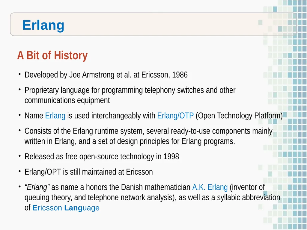
slide3. Erlang A Bit of History Developed by Joe Armstrong et al. at Ericsson, 1986
Proprietary language for programming telephony switches and other communications equipment
Name Erlang is used interchangeably with Erlang/OTP (Open Technology Platform)
Consists of the Erlang runtime system, several ready-to-use components mainly written in Erlang, and a set of design principles for Erlang programs.
Released as free open-source technology in 1998
Erlang/OPT is still maintained at Ericsson
“Erlang” as name a honors the Danish mathematician A.K. Erlang (inventor of queuing theory, and telephone network analysis), as well as a syllabic abbreviation of Ericsson Language<br>
slide4. Erlang Usage Sasa Juric (author) : “Erlang is a development platform for building scalable and reliable systems that constantly provide service with little or no downtime.”
Ericsson’s original need that led to Erlang was telecom systems where properties ike reliability, responsioveness, scalability, and constant availability were imperitive.<br>
slide5. Erlang Usage Tim Bray (Sun Microsystems, 2008: “If somebody came to me and wanted to pay me a lot of money to build a large scale message handling system that really had to be up all the time, could never afford to go down for years at a time, I would unhesitatingly choose Erlang to build it in.”
As of 2014, Erlang was being used in Ericsson nodes, European GPRS networks, 3G and LTE networks worldwide, and by Nortel and T-mobile
WhatsApp is coded in Erlang
Being used in Financial Tech, Gaming, Healthcare, Automotive, IoT and Blockchain platforms, also massively multiple-player online gaming
Used by Vocalink, Goldman Sachs, Nintendo, Samsung, Meta (Facebook)<br>
slide6. Erlang Nature of Erlang Programs The Erlang programming language has
immutable data
pattern matching
functional programming
garbage collection ( and here )
The sequential subset of the Erlang language supports
eager evaluation
single assignment
dynamic typing
A normal Erlang application is built out of hundreds (maybe thousands) of small Erlang processes.<br>
slide7. Erlang BEAM and ERTS BEAM is the virtual machine at the core of the Erlang OTP
BEAM is part of the Erlang Run-Time System ( ERTS ), which compiles Erlang source code into bytecode, which is then run on the BEAM
(wiki) Originally BEAM was short for Bogdan's Erlang Abstract Machine, named after Bogumil "Bogdan" Hausman, who wrote the original version, but the name may also be referred to as Björn's Erlang Abstract Machine, after Björn Gustavsson, who wrote and maintains the current version. Both were done at Ericsson<br>
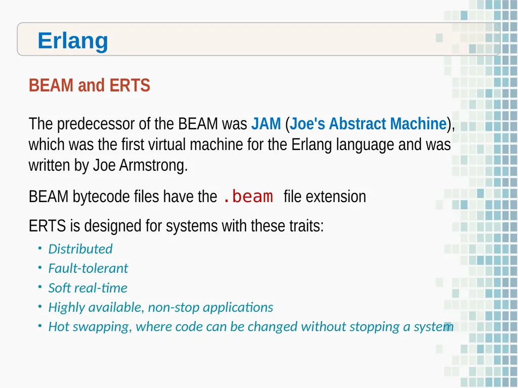
slide8. Erlang BEAM and ERTS The predecessor of the BEAM was JAM (Joe's Abstract Machine), which was the first virtual machine for the Erlang language and was written by Joe Armstrong.
BEAM bytecode files have the .beam file extension
ERTS is designed for systems with these traits:
Distributed
Fault-tolerant
Soft real-time
Highly available, non-stop applications
Hot swapping, where code can be changed without stopping a system<br>
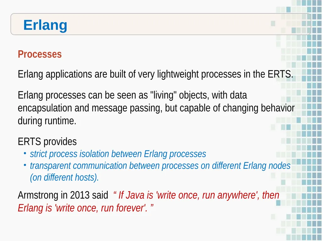
slide9. Erlang Processes Erlang applications are built of very lightweight processes in the ERTS.
Erlang processes can be seen as "living" objects, with data encapsulation and message passing, but capable of changing behavior during runtime.
ERTS provides
strict process isolation between Erlang processes
transparent communication between processes on different Erlang nodes (on different hosts).
Armstrong in 2013 said “ If Java is 'write once, run anywhere', then Erlang is 'write once, run forever'. ”<br>
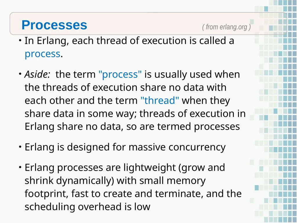
slide10. Processes ( from erlang.org ) In Erlang, each thread of execution is called a process.
Aside: the term "process" is usually used when the threads of execution share no data with each other and the term "thread" when they share data in some way; threads of execution in Erlang share no data, so are termed processes
Erlang is designed for massive concurrency
Erlang processes are lightweight (grow and shrink dynamically) with small memory footprint, fast to create and terminate, and the scheduling overhead is low<br>
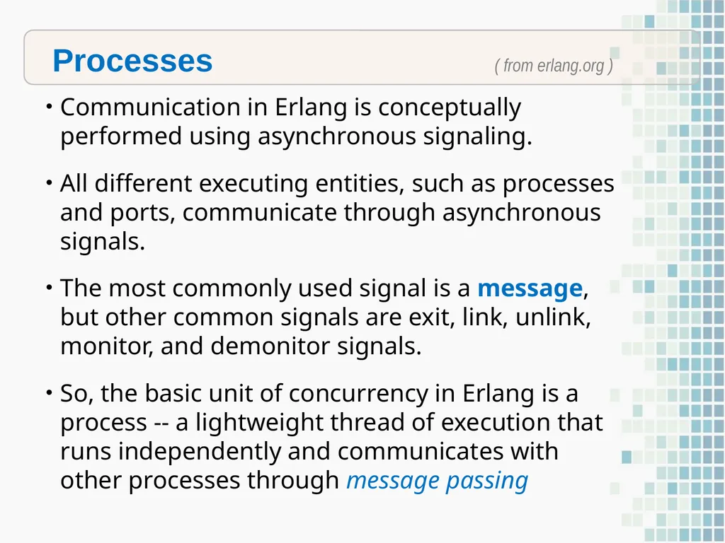
slide11. Processes ( from erlang.org ) Communication in Erlang is conceptually performed using asynchronous signaling.
All different executing entities, such as processes and ports, communicate through asynchronous signals.
The most commonly used signal is a message, but other common signals are exit, link, unlink, monitor, and demonitor signals.
So, the basic unit of concurrency in Erlang is a process -- a lightweight thread of execution that runs independently and communicates with other processes through message passing<br>
slide12. Processes ( from erlang.org ) Processes are created with the spawn function, which takes a function as an argument and returns a process identifier (pid).
An Erlang “program” is a call to an initial function (in a module); that function may spawn other processes… which may spawn more, etc.
Erlang processes operate in (memory) isolation from each other, and are scheduled by Erlang's Virtual Machine (VM).
The creation time of process is very low, the memory footprint of a just spawned process is very small, and a single Erlang VM can have millions of processes running.
The default max number of alive processes is by default 32,768. This limit can be raised up to 268,435,456 processes at startup.<br>
slide13. Erlang Principles of Erlang Processes Everything is a process.
Processes are strongly isolated.
Process creation and destruction is a lightweight operation.
Message passing is the only way for processes to interact.
Processes have unique names.
If you know the name of a process you can send it a message.
Processes share no resources.
Error handling is non-local.
Processes do what they are supposed to do or fail.<br>
slide14. Erlang “Let it crash” or “Let it fail” Erlang supports a "Let it fail" coding style
Has a mechanism that makes it easy for external processes to monitor for crashes (or hardware failures). This is In preference to an in-process mechanism like exception handling used in many other PLs
Crashes are reported like other messages (the only way processes can communicate with each other). Subprocesses can be spawned cheaply
So prefer a process be completely restarted rather than trying to recover from a failure
This philosophy results in less code devoted to defensive programming where error-handling code is highly contextual and specific<br>
slide15. Let it fail …. means “Let it crash” or “Let it fail” Design philosophy: design systems expecting that failure will happen; build a supervisor structure to monitor executions, detect failures, and quickly restart failed processes
Error detection via supervisor infrastructure
Fail fast, then recover
Isolation of failures<br>
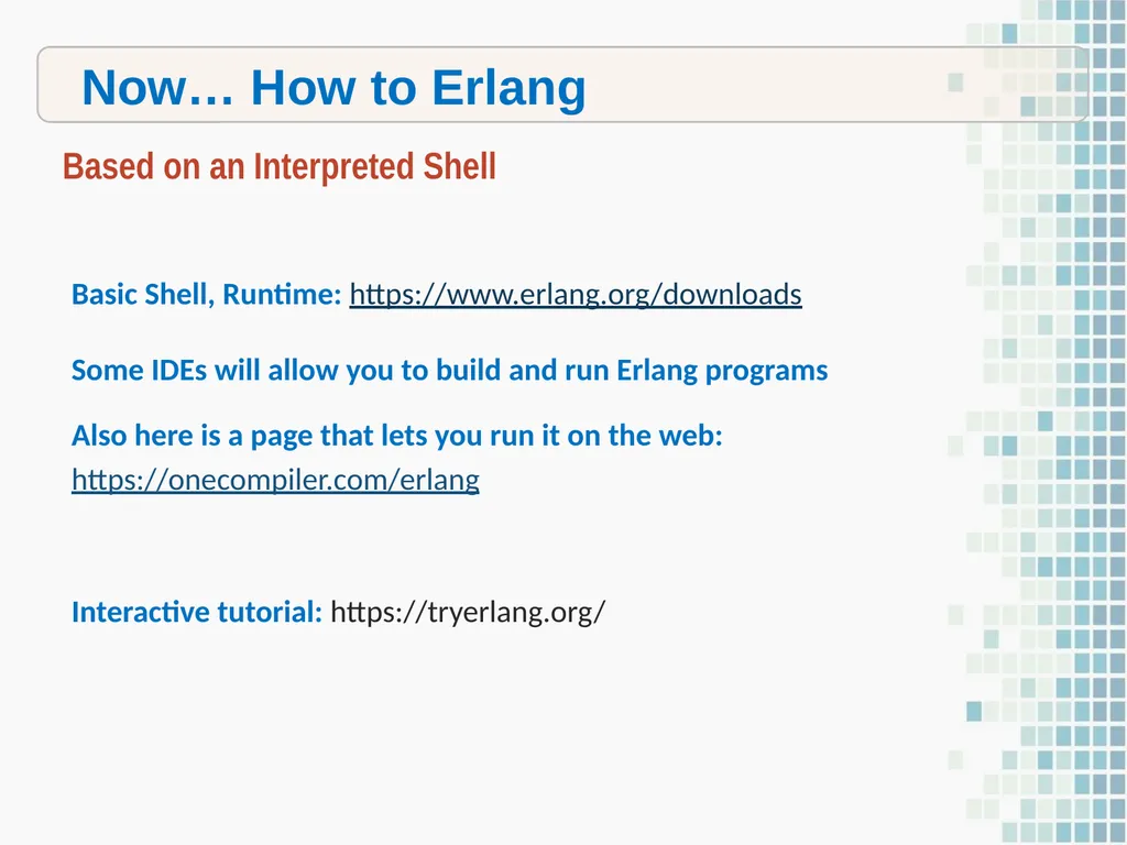
slide16. Now… How to Erlang Based on an Interpreted Shell Basic Shell, Runtime: https://www.erlang.org/downloads
Some IDEs will allow you to build and run Erlang programs
Also here is a page that lets you run it on the web:
https://onecompiler.com/erlang
Interactive tutorial: https://tryerlang.org/<br>
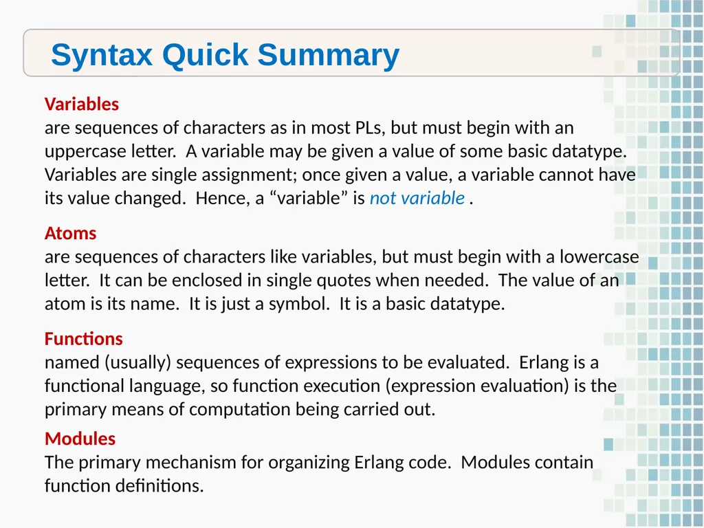
slide17. Syntax Quick Summary Variables
are sequences of characters as in most PLs, but must begin with an uppercase letter. A variable may be given a value of some basic datatype. Variables are single assignment; once given a value, a variable cannot have its value changed. Hence, a “variable” is not variable .
Atoms
are sequences of characters like variables, but must begin with a lowercase letter. It can be enclosed in single quotes when needed. The value of an atom is its name. It is just a symbol. It is a basic datatype.
Functions
named (usually) sequences of expressions to be evaluated. Erlang is a functional language, so function execution (expression evaluation) is the primary means of computation being carried out.
Modules
The primary mechanism for organizing Erlang code. Modules contain function definitions.<br>
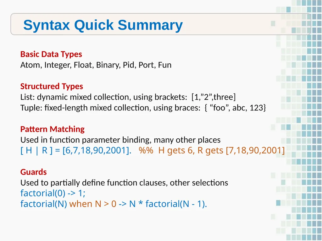
slide18. Syntax Quick Summary Basic Data Types
Atom, Integer, Float, Binary, Pid, Port, Fun
Structured Types
List: dynamic mixed collection, using brackets: [1,”2”,three]
Tuple: fixed-length mixed collection, using braces: { “foo”, abc, 123}
Pattern Matching
Used in function parameter binding, many other places
[ H | R ] = [6,7,18,90,2001]. %% H gets 6, R gets [7,18,90,2001]
Guards
Used to partially define function clauses, other selections
factorial(0) -> 1;
factorial(N) when N > 0 -> N * factorial(N - 1).<br>
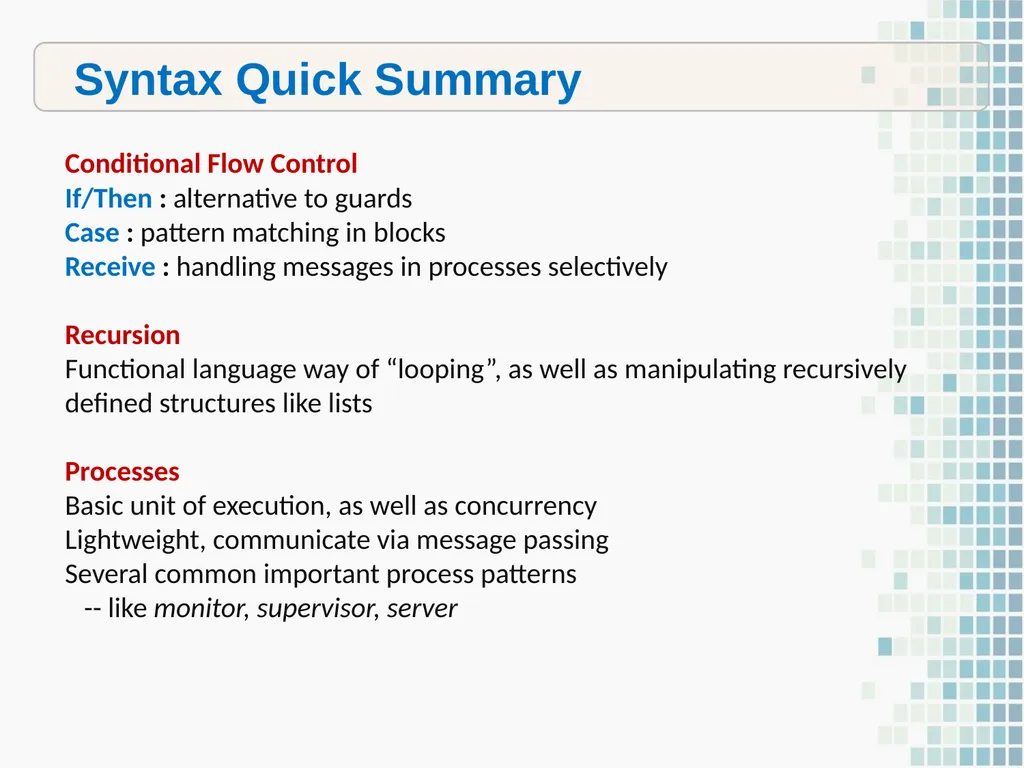
slide19. Syntax Quick Summary Conditional Flow Control
If/Then : alternative to guards
Case : pattern matching in blocks
Receive : handling messages in processes selectively
Recursion
Functional language way of “looping”, as well as manipulating recursively defined structures like lists
Processes
Basic unit of execution, as well as concurrency
Lightweight, communicate via message passing
Several common important process patterns
-- like monitor, supervisor, server<br>
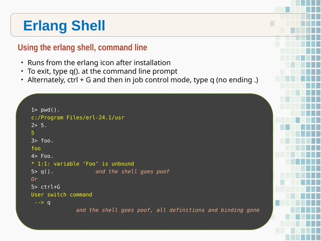
slide20. Erlang Shell Using the erlang shell, command line Runs from the erlang icon after installation
To exit, type q(). at the command line prompt
Alternately, ctrl + G and then in job control mode, type q (no ending .) 1> pwd().
c:/Program Files/erl-24.1/usr
2> 5.
5
3> foo.
foo
4> Foo.
* 1:1: variable ‘Foo’ is unbound
5> q(). and the shell goes poof
Or
5> ctrl+G
User switch command
--> q
and the shell goes poof, all definitions and binding gone<br>
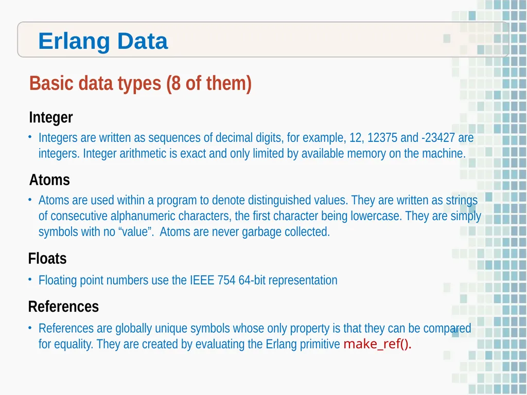
slide21. Erlang Data Basic data types (8 of them) Integer
Integers are written as sequences of decimal digits, for example, 12, 12375 and -23427 are integers. Integer arithmetic is exact and only limited by available memory on the machine.
Atoms
Atoms are used within a program to denote distinguished values. They are written as strings of consecutive alphanumeric characters, the first character being lowercase. They are simply symbols with no “value”. Atoms are never garbage collected.
Floats
Floating point numbers use the IEEE 754 64-bit representation
References
References are globally unique symbols whose only property is that they can be compared for equality. They are created by evaluating the Erlang primitive make_ref().<br>
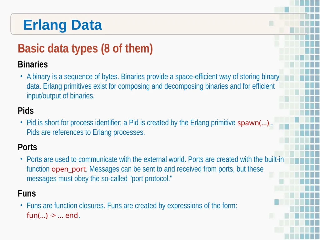
slide22. Erlang Data Basic data types (8 of them) Binaries
A binary is a sequence of bytes. Binaries provide a space-efficient way of storing binary data. Erlang primitives exist for composing and decomposing binaries and for efficient input/output of binaries.
Pids
Pid is short for process identifier; a Pid is created by the Erlang primitive spawn(...) . Pids are references to Erlang processes.
Ports
Ports are used to communicate with the external world. Ports are created with the built-in function open_port. Messages can be sent to and received from ports, but these messages must obey the so-called "port protocol."
Funs
Funs are function closures. Funs are created by expressions of the form: fun(...) -> ... end.<br>
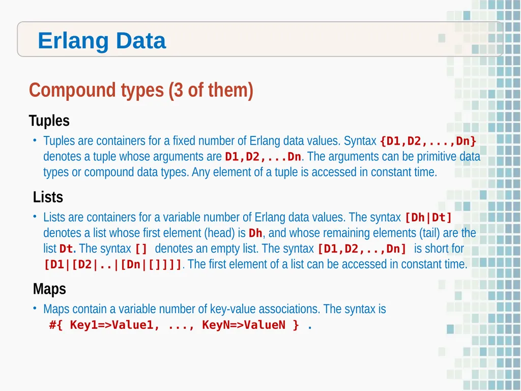
slide23. Erlang Data Compound types (3 of them) Tuples
Tuples are containers for a fixed number of Erlang data values. Syntax {D1,D2,...,Dn} denotes a tuple whose arguments are D1,D2,...Dn. The arguments can be primitive data types or compound data types. Any element of a tuple is accessed in constant time.
Lists
Lists are containers for a variable number of Erlang data values. The syntax [Dh|Dt] denotes a list whose first element (head) is Dh, and whose remaining elements (tail) are the list Dt. The syntax [] denotes an empty list. The syntax [D1,D2,..,Dn] is short for [D1|[D2|..|[Dn|[]]]]. The first element of a list can be accessed in constant time.
Maps
Maps contain a variable number of key-value associations. The syntax is #{ Key1=>Value1, ..., KeyN=>ValueN } .<br>
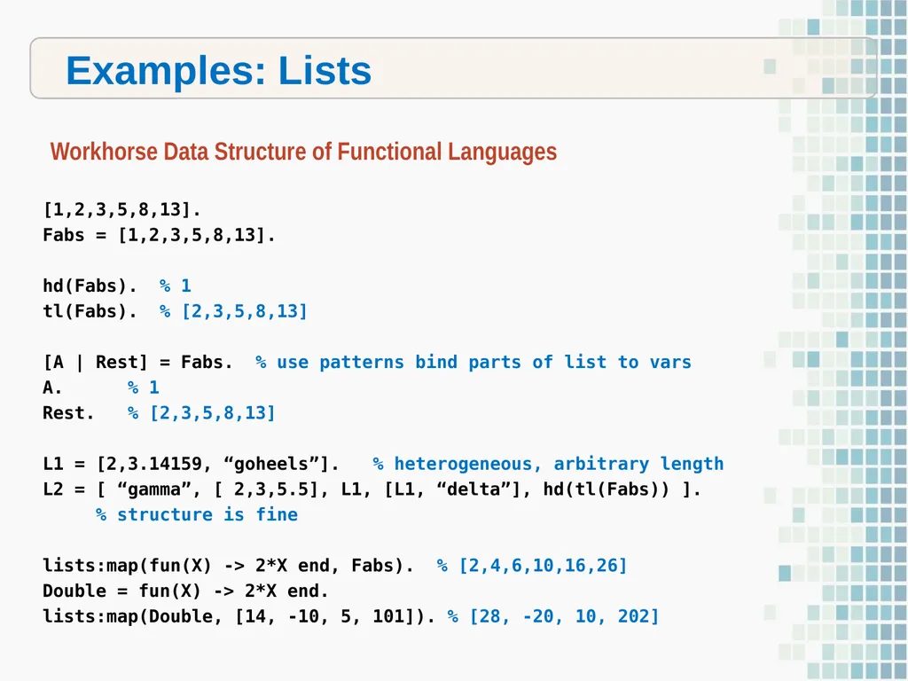
slide24. Examples: Lists Workhorse Data Structure of Functional Languages [1,2,3,5,8,13].
Fabs = [1,2,3,5,8,13].
hd(Fabs). % 1
tl(Fabs). % [2,3,5,8,13]
[A | Rest] = Fabs. % use patterns bind parts of list to vars
A. % 1
Rest. % [2,3,5,8,13]
L1 = [2,3.14159, “goheels”]. % heterogeneous, arbitrary length
L2 = [ “gamma”, [ 2,3,5.5], L1, [L1, “delta”], hd(tl(Fabs)) ].
% structure is fine
lists:map(fun(X) -> 2*X end, Fabs). % [2,4,6,10,16,26]
Double = fun(X) -> 2*X end.
lists:map(Double, [14, -10, 5, 101]). % [28, -20, 10, 202]<br>
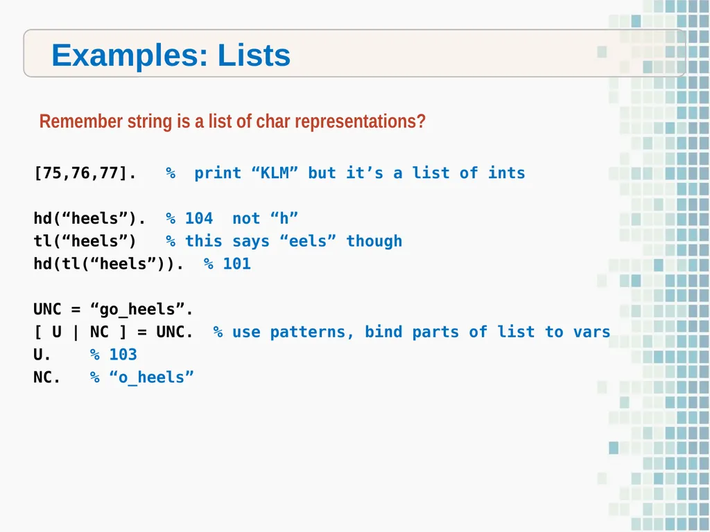
slide25. Examples: Lists Remember string is a list of char representations? [75,76,77]. % print “KLM” but it’s a list of ints
hd(“heels”). % 104 not “h”
tl(“heels”) % this says “eels” though
hd(tl(“heels”)). % 101
UNC = “go_heels”.
[ U | NC ] = UNC. % use patterns, bind parts of list to vars
U. % 103
NC. % “o_heels”<br>
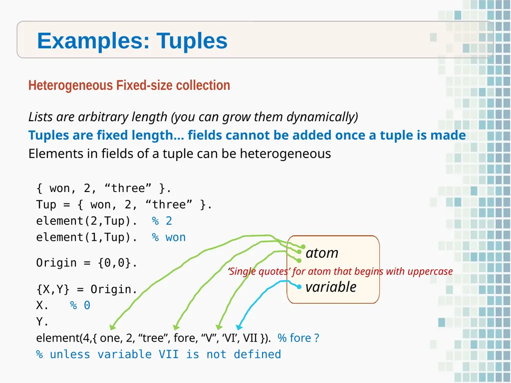
slide26. Examples: Tuples Heterogeneous Fixed-size collection Lists are arbitrary length (you can grow them dynamically)
Tuples are fixed length… fields cannot be added once a tuple is made
Elements in fields of a tuple can be heterogeneous { won, 2, “three” }.
Tup = { won, 2, “three” }.
element(2,Tup). % 2
element(1,Tup). % won
Origin = {0,0}.
{X,Y} = Origin.
X. % 0
Y.
element(4,{ one, 2, “tree”, fore, “V”, ‘VI’, VII }). % fore ?
% unless variable VII is not defined ‘Single quotes’ for atom that begins with uppercase<br>
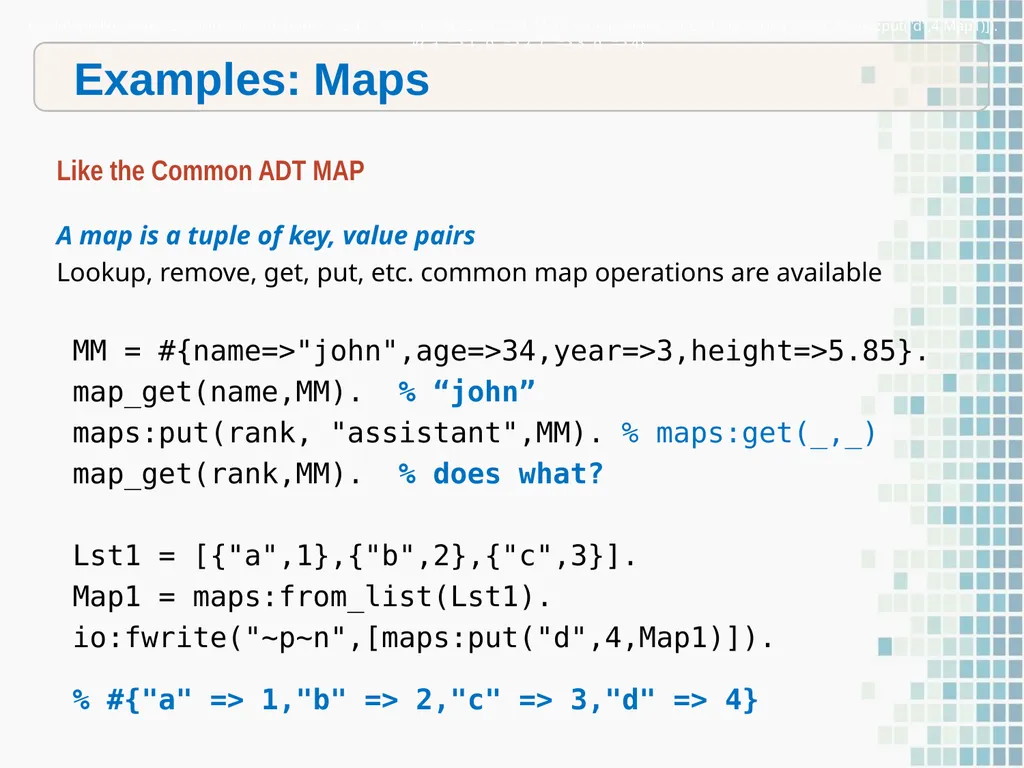
slide27. Examples: Maps Like the Common ADT MAP A map is a tuple of key, value pairs
Lookup, remove, get, put, etc. common map operations are available MM = #{name=>"john",age=>34,year=>3,height=>5.85}.
map_get(name,MM). % “john”
maps:put(rank, "assistant",MM). % maps:get(_,_)
map_get(rank,MM). % does what?
Lst1 = [{"a",1},{"b",2},{"c",3}].
Map1 = maps:from_list(Lst1).
io:fwrite("~p~n",[maps:put("d",4,Map1)]).
% #{"a" => 1,"b" => 2,"c" => 3,"d" => 4} -module(helloworld). -export([start/0]). start() -> Lst1 = [{"a",1},{"b",2},{"c",3}], Map1 = maps:from_list(Lst1), io:fwrite("~p~n",[maps:put("d",4,Map1)]). #{"a" => 1,"b" => 2,"c" => 3,"d" => 4}<br>
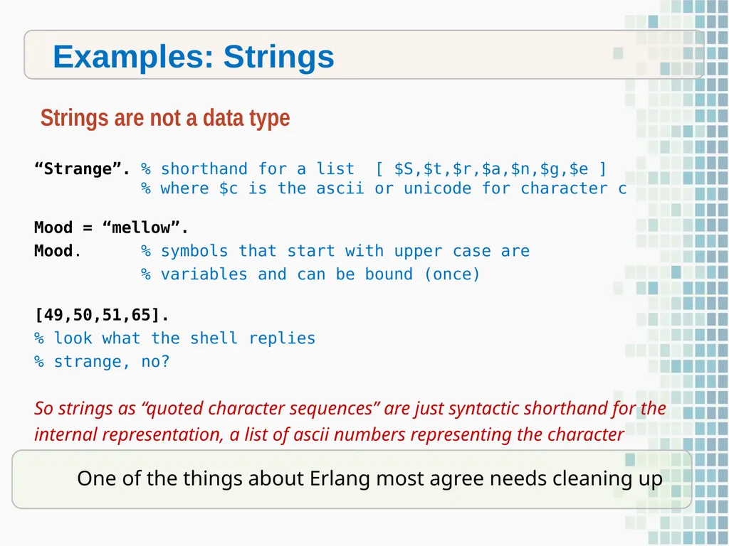
slide28. Examples: Strings Strings are not a data type “Strange”. % shorthand for a list [ $S,$t,$r,$a,$n,$g,$e ]
% where $c is the ascii or unicode for character c
Mood = “mellow”.
Mood. % symbols that start with upper case are
% variables and can be bound (once)
[49,50,51,65].
% look what the shell replies
% strange, no?
So strings as “quoted character sequences” are just syntactic shorthand for the internal representation, a list of ascii numbers representing the character
One of the things about Erlang most agree needs cleaning up<br>
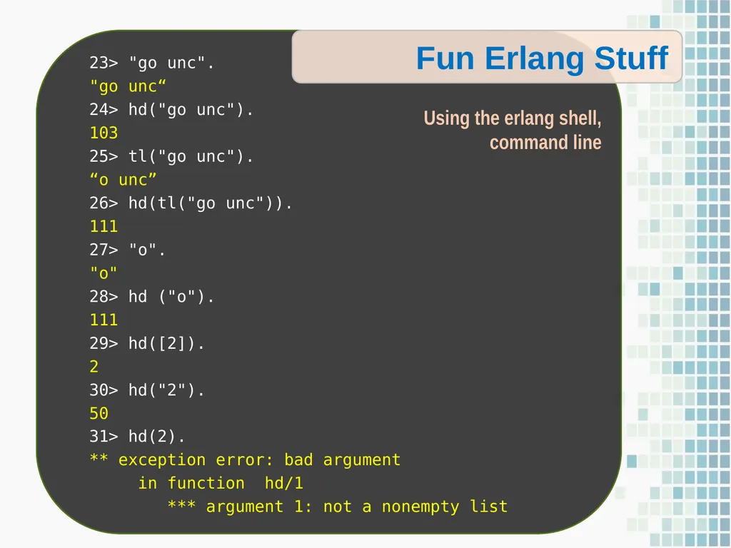
slide29. 23> "go unc".
"go unc“
24> hd("go unc").
103
25> tl("go unc").
“o unc”
26> hd(tl("go unc")).
111
27> "o".
"o"
28> hd ("o").
111
29> hd([2]).
2
30> hd("2").
50
31> hd(2).
** exception error: bad argument
in function hd/1
*** argument 1: not a nonempty list Using the erlang shell, command line Fun Erlang Stuff<br>
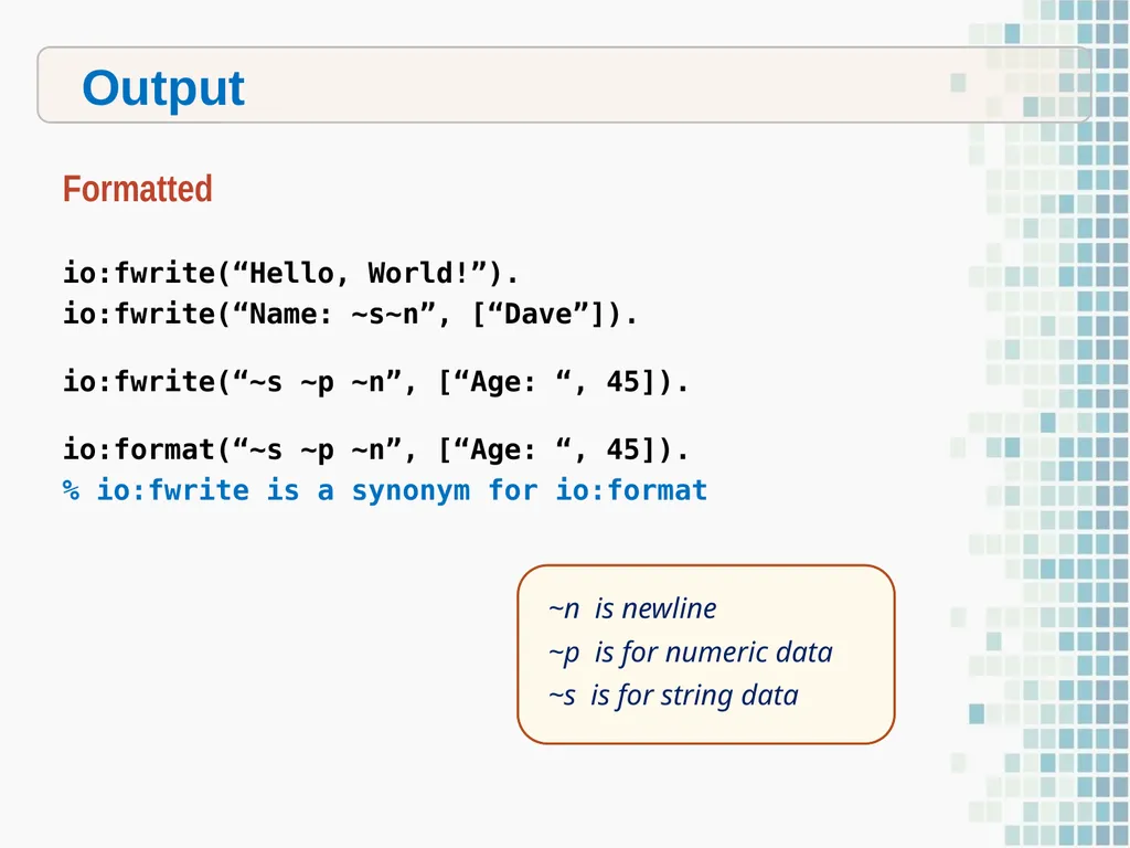
slide30. io:fwrite(“Hello, World!”).
io:fwrite(“Name: ~s~n”, [“Dave”]).
io:fwrite(“~s ~p ~n”, [“Age: “, 45]).
io:format(“~s ~p ~n”, [“Age: “, 45]).
% io:fwrite is a synonym for io:format Output Formatted<br>
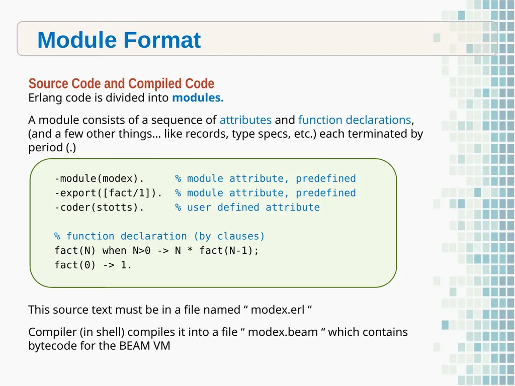
slide31. Module Format Source Code and Compiled Code Erlang code is divided into modules.
A module consists of a sequence of attributes and function declarations, (and a few other things… like records, type specs, etc.) each terminated by period (.) -module(modex). % module attribute, predefined
-export([fact/1]). % module attribute, predefined
-coder(stotts). % user defined attribute
% function declaration (by clauses)
fact(N) when N>0 -> N * fact(N-1);
fact(0) -> 1. This source text must be in a file named “ modex.erl “
Compiler (in shell) compiles it into a file “ modex.beam “ which contains bytecode for the BEAM VM<br>
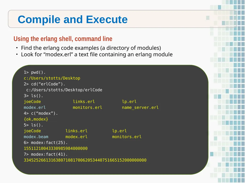
slide32. Compile and Execute Using the erlang shell, command line Find the erlang code examples (a directory of modules)
Look for “modex.erl” a text file containing an erlang module 1> pwd().
c:/Users/stotts/Desktop
2> cd(“erlCode”).
c:/Users/stotts/Desktop/erlCode
3> ls().
joeCode links.erl lp.erl
modex.erl monitors.erl name_server.erl
4> c(“modex”).
{ok,modex}
5> ls().
joeCode links.erl lp.erl
modex.beam modex.erl monitors.erl
6> modex:fact(25).
15511210043330985984000000
7> modex:fact(41).
33452526613163807108170062053440751665152000000000<br>
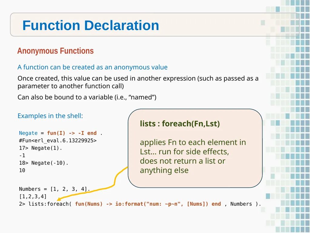
slide33. Function Declaration Anonymous Functions A function can be created as an anonymous value
Once created, this value can be used in another expression (such as passed as a parameter to another function call)
Can also be bound to a variable (i.e., “named”) Negate = fun(I) -> -I end .
#Fun<erl_eval.6.13229925>
17> Negate(1).
-1
18> Negate(-10).
10
Numbers = [1, 2, 3, 4].
[1,2,3,4]
2> lists:foreach( fun(Nums) -> io:format("num: ~p~n", [Nums]) end , Numbers ). Examples in the shell:<br>
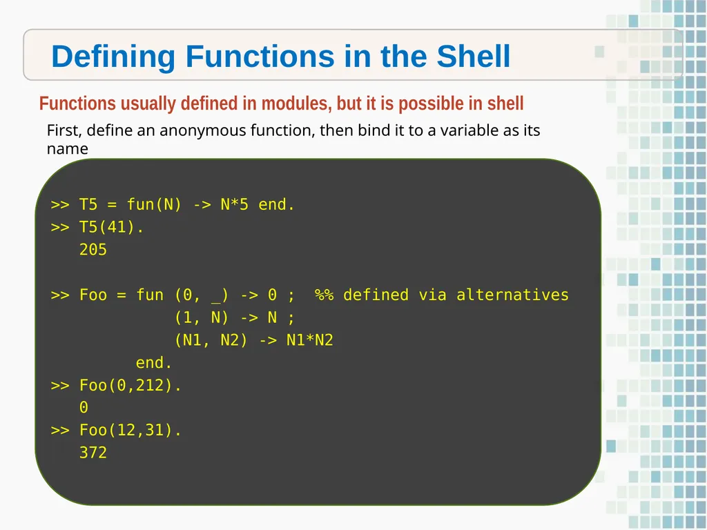
slide34. Defining Functions in the Shell Functions usually defined in modules, but it is possible in shell First, define an anonymous function, then bind it to a variable as its name >> T5 = fun(N) -> N*5 end.
>> T5(41).
205
>> Foo = fun (0, _) -> 0 ; %% defined via alternatives
(1, N) -> N ;
(N1, N2) -> N1*N2
end.
>> Foo(0,212).
0
>> Foo(12,31).
372<br>
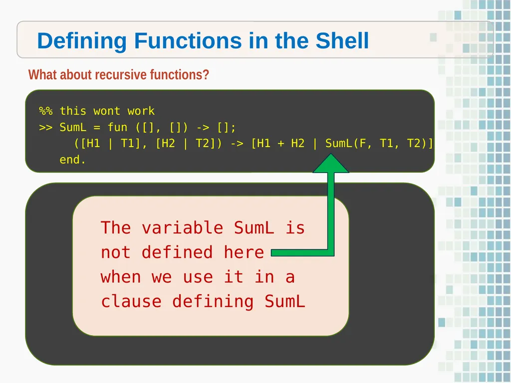
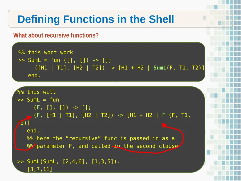
slide35. Defining Functions in the Shell What about recursive functions? %% this wont work
>> SumL = fun ([], []) -> [];
([H1 | T1], [H2 | T2]) -> [H1 + H2 | SumL(F, T1, T2)]
end. The variable SumL is not defined here
when we use it in a clause defining SumL<br>
slide36. Defining Functions in the Shell What about recursive functions? %% this will
>> SumL = fun
(F, [], []) -> [];
(F, [H1 | T1], [H2 | T2]) -> [H1 + H2 | F (F, T1, T2)]
end.
%% here the “recursive” func is passed in as a
%% parameter F, and called in the second clause
>> SumL(SumL, [2,4,6], [1,3,5]).
[3,7,11] %% this wont work
>> SumL = fun ([], []) -> [];
([H1 | T1], [H2 | T2]) -> [H1 + H2 | SumL(F, T1, T2)]
end.<br>
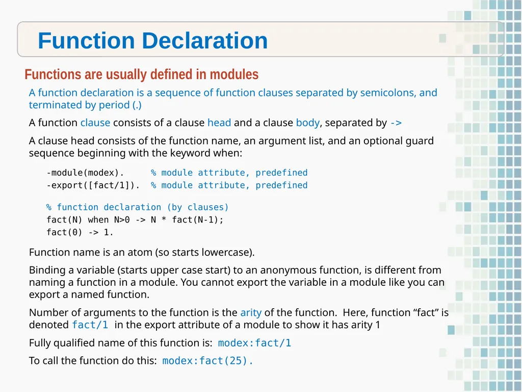
slide37. Function Declaration A function declaration is a sequence of function clauses separated by semicolons, and terminated by period (.)
A function clause consists of a clause head and a clause body, separated by ->
A clause head consists of the function name, an argument list, and an optional guard sequence beginning with the keyword when: -module(modex). % module attribute, predefined
-export([fact/1]). % module attribute, predefined
% function declaration (by clauses)
fact(N) when N>0 -> N * fact(N-1);
fact(0) -> 1. Function name is an atom (so starts lowercase).
Binding a variable (starts upper case start) to an anonymous function, is different from naming a function in a module. You cannot export the variable in a module like you can export a named function.
Number of arguments to the function is the arity of the function. Here, function “fact” is denoted fact/1 in the export attribute of a module to show it has arity 1
Fully qualified name of this function is: modex:fact/1
To call the function do this: modex:fact(25). Functions are usually defined in modules<br>
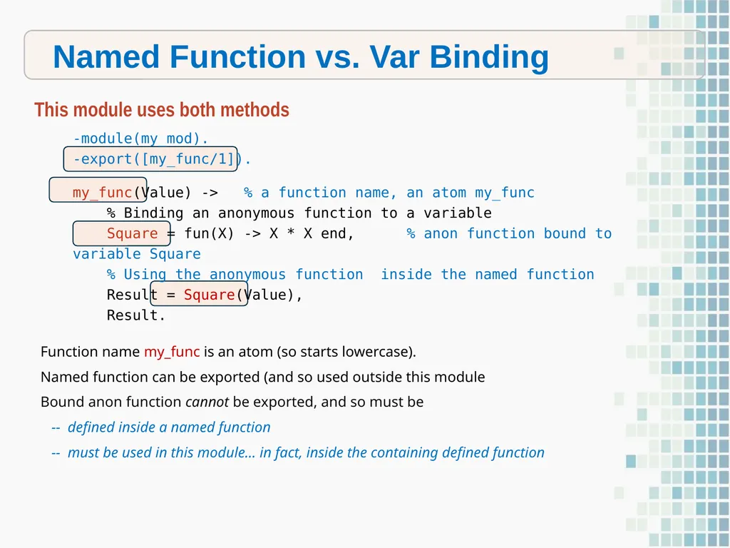
slide38. -module(my_mod).
-export([my_func/1]).
my_func(Value) -> % a function name, an atom my_func
% Binding an anonymous function to a variable
Square = fun(X) -> X * X end, % anon function bound to variable Square
% Using the anonymous function inside the named function
Result = Square(Value),
Result. Named Function vs. Var Binding Function name my_func is an atom (so starts lowercase).
Named function can be exported (and so used outside this module
Bound anon function cannot be exported, and so must be
-- defined inside a named function
-- must be used in this module… in fact, inside the containing defined function This module uses both methods<br>
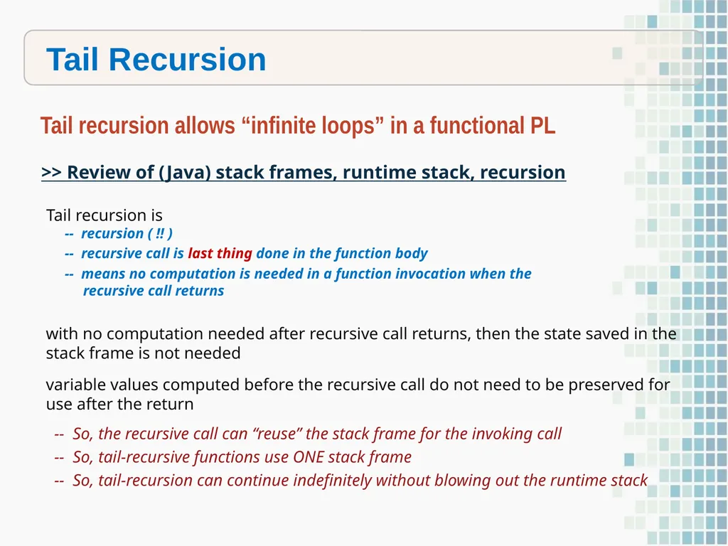
slide39. Tail Recursion Tail recursion allows “infinite loops” in a functional PL >> Review of (Java) stack frames, runtime stack, recursion Tail recursion is
-- recursion ( !! )
-- recursive call is last thing done in the function body
-- means no computation is needed in a function invocation when the
recursive call returns with no computation needed after recursive call returns, then the state saved in the stack frame is not needed
variable values computed before the recursive call do not need to be preserved for use after the return
-- So, the recursive call can “reuse” the stack frame for the invoking call
-- So, tail-recursive functions use ONE stack frame
-- So, tail-recursion can continue indefinitely without blowing out the runtime stack<br>
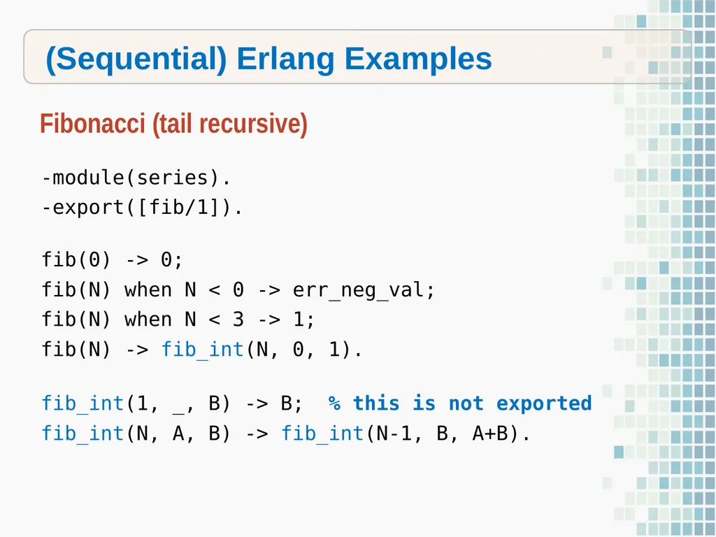
slide40. (Sequential) Erlang Examples Fibonacci (tail recursive) -module(series).
-export([fib/1]).
fib(0) -> 0;
fib(N) when N < 0 -> err_neg_val;
fib(N) when N < 3 -> 1;
fib(N) -> fib_int(N, 0, 1).
fib_int(1, _, B) -> B; % this is not exported
fib_int(N, A, B) -> fib_int(N-1, B, A+B).<br>
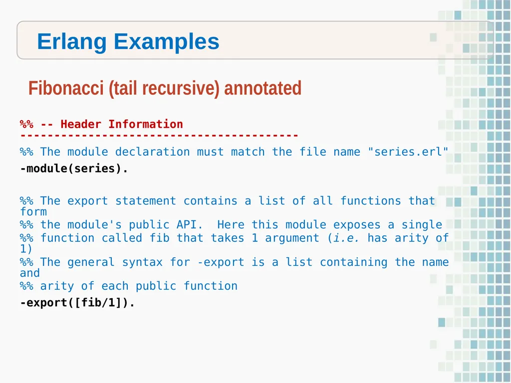
slide41. Erlang Examples Fibonacci (tail recursive) annotated %% -- Header Information -----------------------------------------
%% The module declaration must match the file name "series.erl"
-module(series).
%% The export statement contains a list of all functions that form
%% the module's public API. Here this module exposes a single
%% function called fib that takes 1 argument (i.e. has arity of 1)
%% The general syntax for -export is a list containing the name and
%% arity of each public function
-export([fib/1]).<br>
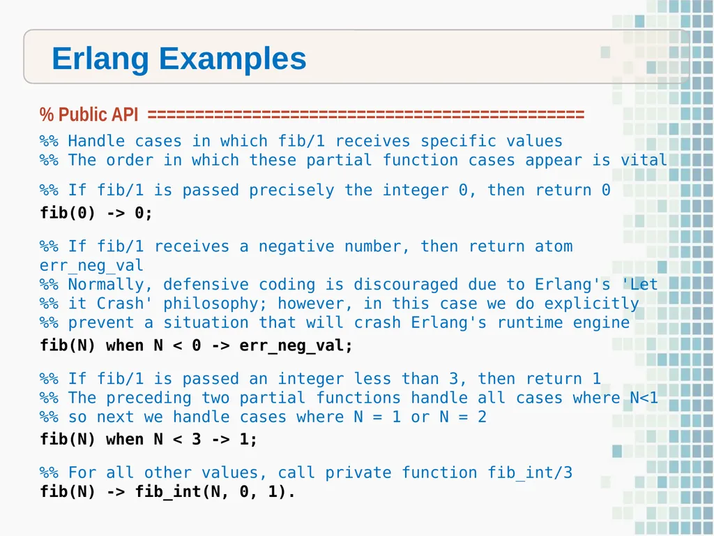
slide42. Erlang Examples % Public API ============================================== %% Handle cases in which fib/1 receives specific values
%% The order in which these partial function cases appear is vital
%% If fib/1 is passed precisely the integer 0, then return 0
fib(0) -> 0;
%% If fib/1 receives a negative number, then return atom err_neg_val
%% Normally, defensive coding is discouraged due to Erlang's 'Let
%% it Crash' philosophy; however, in this case we do explicitly
%% prevent a situation that will crash Erlang's runtime engine
fib(N) when N < 0 -> err_neg_val;
%% If fib/1 is passed an integer less than 3, then return 1
%% The preceding two partial functions handle all cases where N<1
%% so next we handle cases where N = 1 or N = 2
fib(N) when N < 3 -> 1;
%% For all other values, call private function fib_int/3
fib(N) -> fib_int(N, 0, 1).<br>
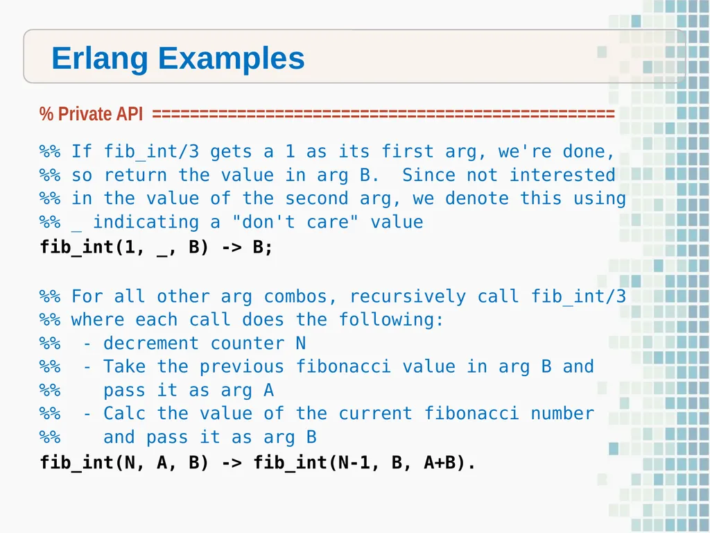
slide43. Erlang Examples % Private API ================================================= %% If fib_int/3 gets a 1 as its first arg, we're done,
%% so return the value in arg B. Since not interested
%% in the value of the second arg, we denote this using
%% _ indicating a "don't care" value
fib_int(1, _, B) -> B;
%% For all other arg combos, recursively call fib_int/3
%% where each call does the following:
%% - decrement counter N
%% - Take the previous fibonacci value in arg B and
%% pass it as arg A
%% - Calc the value of the current fibonacci number
%% and pass it as arg B
fib_int(N, A, B) -> fib_int(N-1, B, A+B).<br>
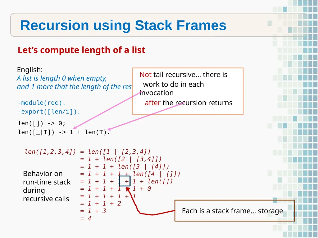
slide44. Recursion using Stack Frames -module(rec).
-export([len/1]).
len([]) -> 0;
len([_|T]) -> 1 + len(T). Let’s compute length of a list English:
A list is length 0 when empty,
and 1 more that the length of the rest of the list when not empty. len([1,2,3,4]) = len([1 | [2,3,4])
= 1 + len([2 | [3,4]])
= 1 + 1 + len([3 | [4]])
= 1 + 1 + 1 + len([4 | []])
= 1 + 1 + 1 + 1 + len([])
= 1 + 1 + 1 + 1 + 0
= 1 + 1 + 1 + 1
= 1 + 1 + 2
= 1 + 3
= 4 Behavior on run-time stack during recursive calls Each is a stack frame… storage Not tail recursive… there is
work to do in each invocation
after the recursion returns<br>
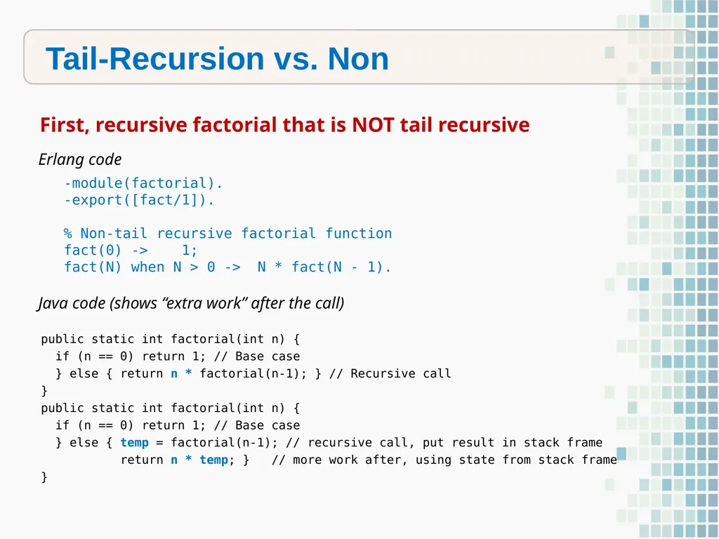
slide45. Tail-Recursion vs. Non -module(factorial).
-export([fact/1]).
% Non-tail recursive factorial function
fact(0) -> 1;
fact(N) when N > 0 -> N * fact(N - 1). First, recursive factorial that is NOT tail recursive Erlang code public static int factorial(int n) {
if (n == 0) return 1; // Base case
} else { return n * factorial(n-1); } // Recursive call
}
public static int factorial(int n) {
if (n == 0) return 1; // Base case
} else { temp = factorial(n-1); // recursive call, put result in stack frame
return n * temp; } // more work after, using state from stack frame
} Java code (shows “extra work” after the call)<br>
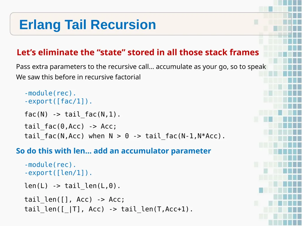
slide46. Erlang Tail Recursion -module(rec).
-export([fac/1]).
fac(N) -> tail_fac(N,1).
tail_fac(0,Acc) -> Acc;
tail_fac(N,Acc) when N > 0 -> tail_fac(N-1,N*Acc). Let’s eliminate the “state” stored in all those stack frames Pass extra parameters to the recursive call… accumulate as your go, so to speak
We saw this before in recursive factorial So do this with len… add an accumulator parameter -module(rec).
-export([len/1]).
len(L) -> tail_len(L,0).
tail_len([], Acc) -> Acc;
tail_len([_|T], Acc) -> tail_len(T,Acc+1).<br>
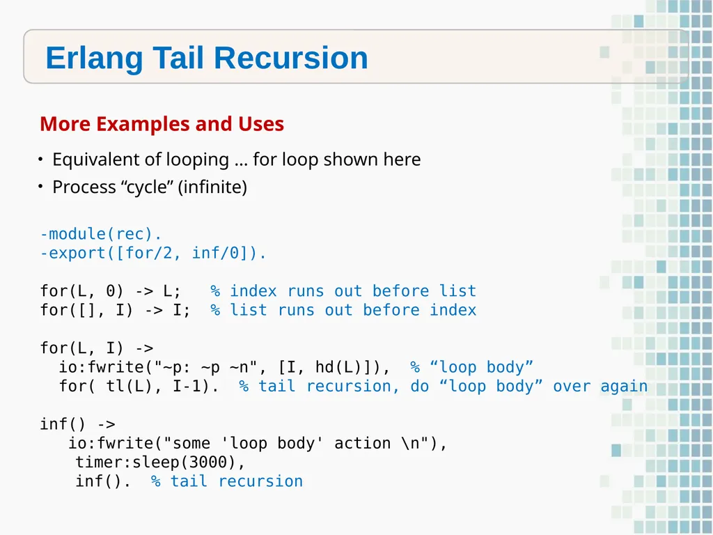
slide47. Erlang Tail Recursion -module(rec).
-export([for/2, inf/0]).
for(L, 0) -> L; % index runs out before list
for([], I) -> I; % list runs out before index
for(L, I) ->
io:fwrite("~p: ~p ~n", [I, hd(L)]), % “loop body”
for( tl(L), I-1). % tail recursion, do “loop body” over again
inf() ->
io:fwrite("some 'loop body' action \n"),
timer:sleep(3000),
inf(). % tail recursion More Examples and Uses Equivalent of looping … for loop shown here
Process “cycle” (infinite)<br>
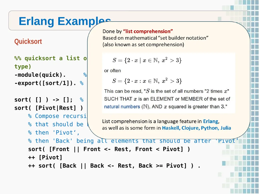
slide48. Erlang Examples Quicksort %% quicksort a list of elements (as long as ‘<‘ is defined for the type)
-module(quick). % This is the file ‘quick.erl'
-export([sort/1]). % fun 'sort' with 1 parm (no type, no name)
sort( [] ) -> []; % If empty list, return empty (nothing to sort)
sort( [Pivot|Rest] ) ->
% Compose recursively a list with 'Front' being all elements
% that should be before 'Pivot‘,
% then 'Pivot‘,
% then 'Back' being all elements that should be after 'Pivot’
sort( [Front || Front <- Rest, Front < Pivot] )
++ [Pivot]
++ sort( [Back || Back <- Rest, Back >= Pivot] ) .<br>
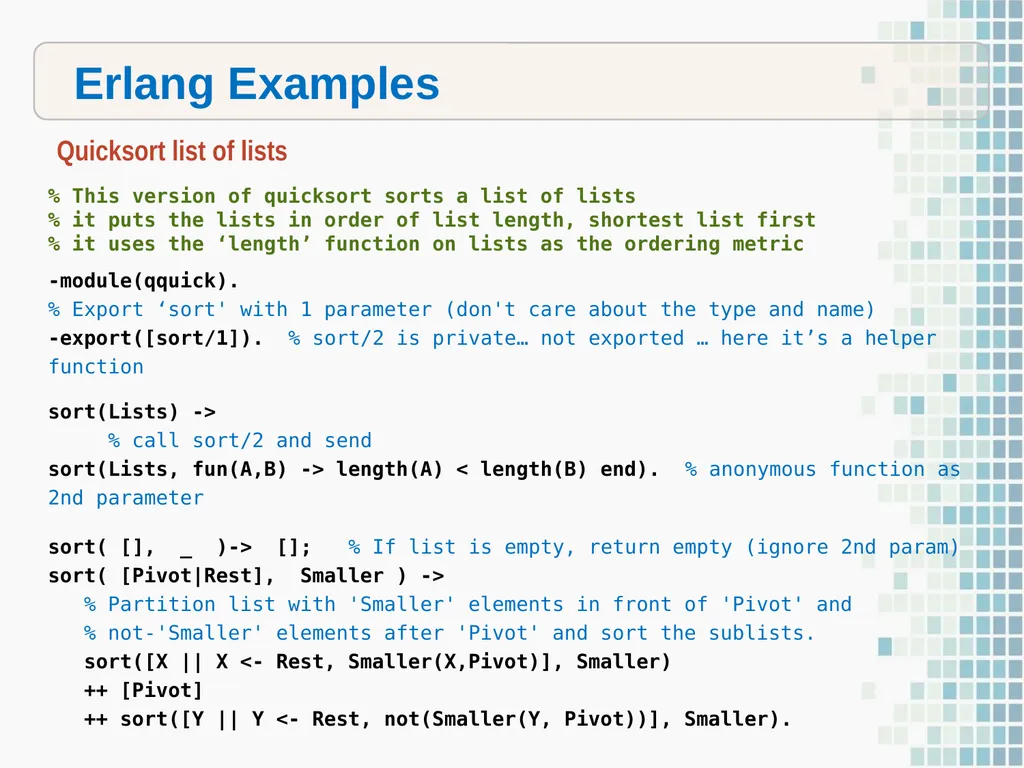
slide49. Erlang Examples Quicksort list of lists % This version of quicksort sorts a list of lists
% it puts the lists in order of list length, shortest list first
% it uses the ‘length’ function on lists as the ordering metric
-module(qquick).
% Export ‘sort' with 1 parameter (don't care about the type and name)
-export([sort/1]). % sort/2 is private… not exported … here it’s a helper function
sort(Lists) -> % call sort/2 and send
sort(Lists, fun(A,B) -> length(A) < length(B) end). % anonymous function as 2nd parameter
sort( [], _ )-> []; % If list is empty, return empty (ignore 2nd param)
sort( [Pivot|Rest], Smaller ) ->
% Partition list with 'Smaller' elements in front of 'Pivot' and
% not-'Smaller' elements after 'Pivot' and sort the sublists.
sort([X || X <- Rest, Smaller(X,Pivot)], Smaller)
++ [Pivot]
++ sort([Y || Y <- Rest, not(Smaller(Y, Pivot))], Smaller).<br>
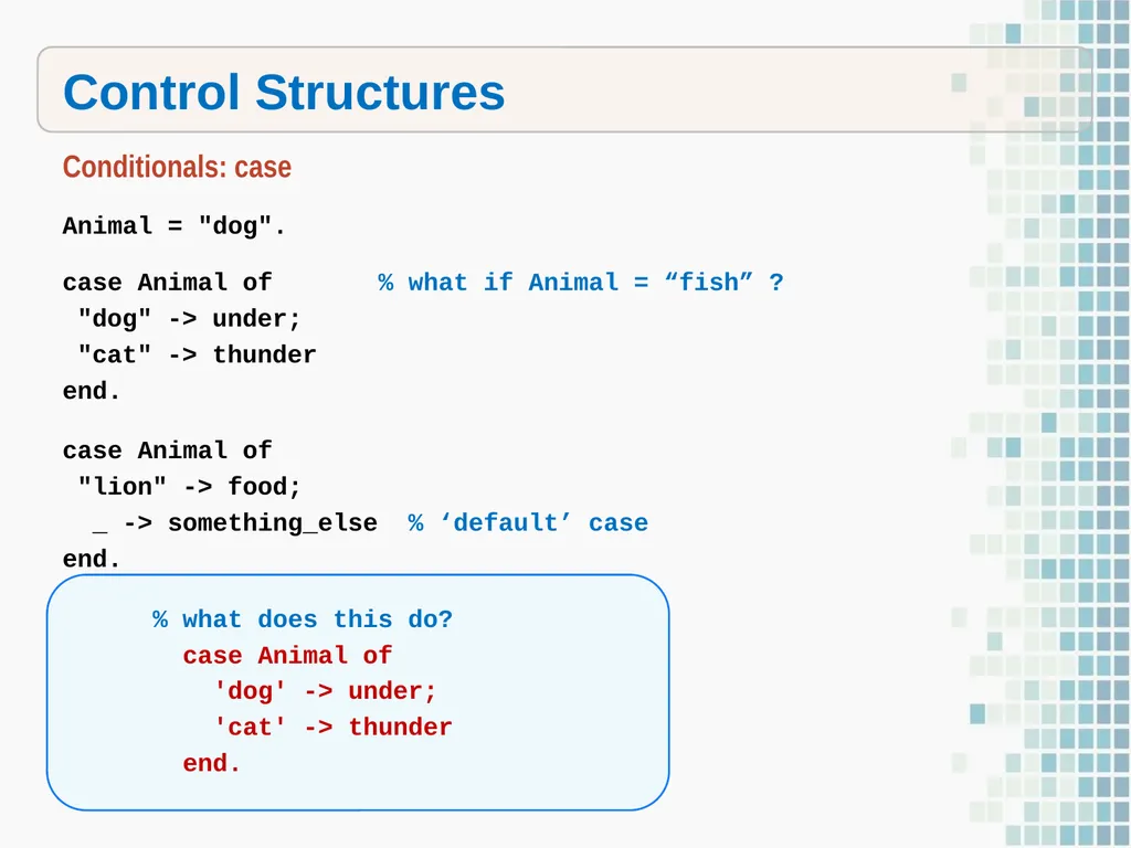
slide50. Control Structures Conditionals: case Animal = "dog".
case Animal of % what if Animal = “fish” ?
"dog" -> under;
"cat" -> thunder
end.
case Animal of
"lion" -> food;
_ -> something_else % ‘default’ case
end.
% what does this do?
case Animal of
'dog' -> under;
'cat' -> thunder
end.<br>
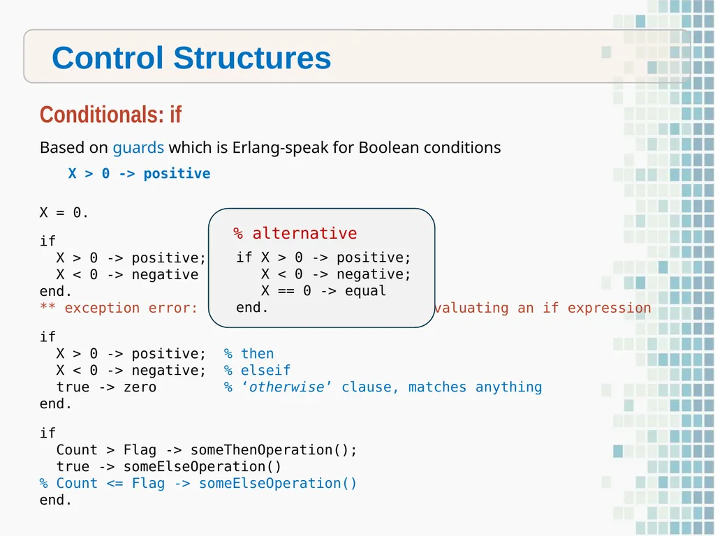
slide51. Control Structures Conditionals: if X = 0.
if
X > 0 -> positive;
X < 0 -> negative
end.
** exception error: no true branch found when evaluating an if expression
if
X > 0 -> positive; % then
X < 0 -> negative; % elseif
true -> zero % ‘otherwise’ clause, matches anything
end.
if
Count > Flag -> someThenOperation();
true -> someElseOperation()
% Count <= Flag -> someElseOperation()
end. Based on guards which is Erlang-speak for Boolean conditions
X > 0 -> positive<br>
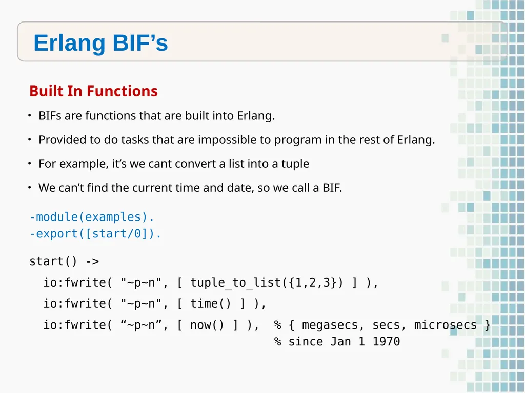
slide52. Erlang BIF’s -module(examples).
-export([start/0]).
start() ->
io:fwrite( "~p~n", [ tuple_to_list({1,2,3}) ] ),
io:fwrite( "~p~n", [ time() ] ),
io:fwrite( “~p~n”, [ now() ] ), % { megasecs, secs, microsecs }
% since Jan 1 1970 Built In Functions BIFs are functions that are built into Erlang.
Provided to do tasks that are impossible to program in the rest of Erlang.
For example, it’s we cant convert a list into a tuple
We can’t find the current time and date, so we call a BIF.<br>
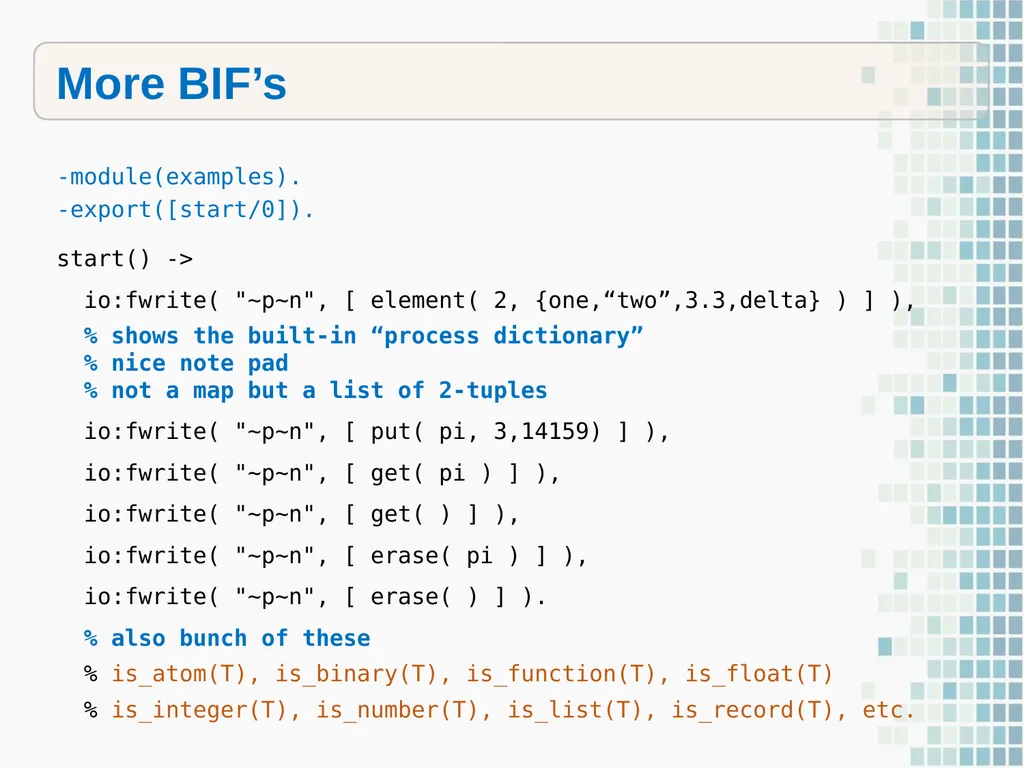
slide53. More BIF’s -module(examples).
-export([start/0]).
start() ->
io:fwrite( "~p~n", [ element( 2, {one,“two”,3.3,delta} ) ] ),
% shows the built-in “process dictionary”
% nice note pad
% not a map but a list of 2-tuples
io:fwrite( "~p~n", [ put( pi, 3,14159) ] ),
io:fwrite( "~p~n", [ get( pi ) ] ),
io:fwrite( "~p~n", [ get( ) ] ),
io:fwrite( "~p~n", [ erase( pi ) ] ),
io:fwrite( "~p~n", [ erase( ) ] ).
% also bunch of these
% is_atom(T), is_binary(T), is_function(T), is_float(T)
% is_integer(T), is_number(T), is_list(T), is_record(T), etc.<br>
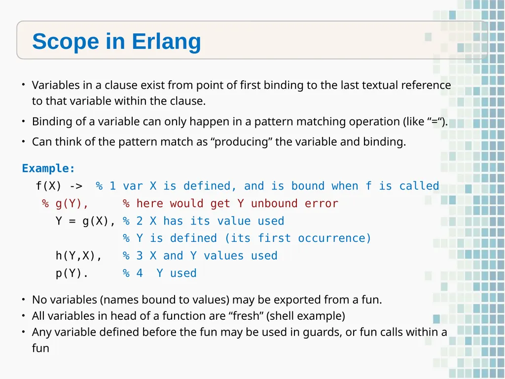
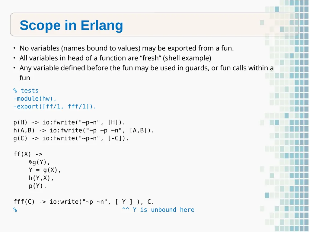
slide54. Scope in Erlang Variables in a clause exist from point of first binding to the last textual reference to that variable within the clause.
Binding of a variable can only happen in a pattern matching operation (like “=“).
Can think of the pattern match as “producing” the variable and binding. Example:
f(X) -> % 1 var X is defined, and is bound when f is called
% g(Y), % here would get Y unbound error
Y = g(X), % 2 X has its value used
% Y is defined (its first occurrence)
h(Y,X), % 3 X and Y values used
p(Y). % 4 Y used No variables (names bound to values) may be exported from a fun.
All variables in head of a function are “fresh” (shell example)
Any variable defined before the fun may be used in guards, or fun calls within a fun<br>
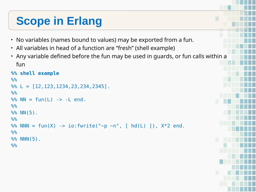
slide55. Scope in Erlang %% shell example
%%
%% L = [12,123,1234,23,234,2345].
%%
%% NN = fun(L) -> -L end.
%%
%% NN(5).
%%
%% NNN = fun(X) -> io:fwrite("~p ~n", [ hd(L) ]), X*2 end.
%%
%% NNN(5).
%% No variables (names bound to values) may be exported from a fun.
All variables in head of a function are “fresh” (shell example)
Any variable defined before the fun may be used in guards, or fun calls within a fun<br>
slide56. Scope in Erlang % tests
-module(hw).
-export([ff/1, fff/1]).
p(H) -> io:fwrite("~p~n", [H]).
h(A,B) -> io:fwrite("~p ~p ~n", [A,B]).
g(C) -> io:fwrite("~p~n", [-C]).
ff(X) ->
%g(Y),
Y = g(X),
h(Y,X),
p(Y).
fff(C) -> io:write("~p ~n", [ Y ] ), C.
% ^^ Y is unbound here No variables (names bound to values) may be exported from a fun.
All variables in head of a function are “fresh” (shell example)
Any variable defined before the fun may be used in guards, or fun calls within a fun<br>
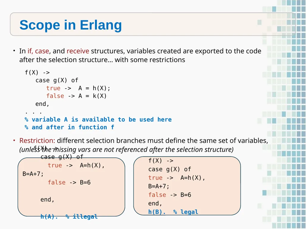
slide57. Scope in Erlang In if, case, and receive structures, variables created are exported to the code after the selection structure… with some restrictions f(X) ->
case g(X) of
true -> A = h(X);
false -> A = k(X)
end,
. . .
% variable A is available to be used here
% and after in function f Restriction: different selection branches must define the same set of variables, (unless the missing vars are not referenced after the selection structure) f(X) ->
case g(X) of
true -> A=h(X), B=A+7;
false -> B=6
end,
h(A). % illegal f(X) ->
case g(X) of
true -> A=h(X), B=A+7;
false -> B=6
end,
h(B). % legal<br>
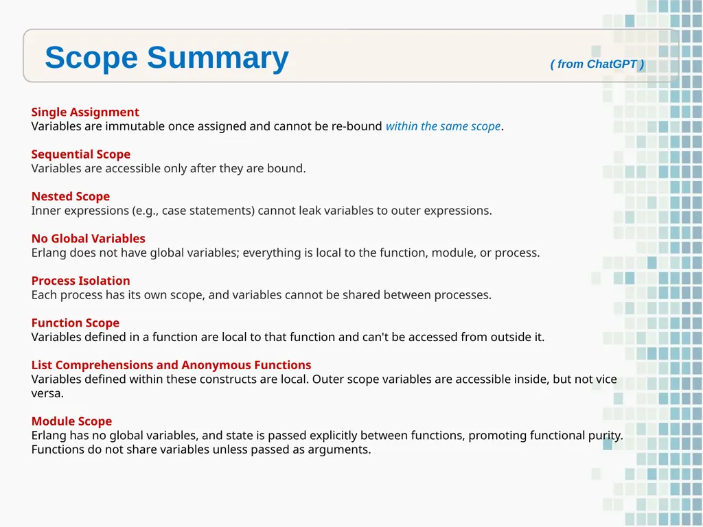
slide58. Scope Summary ( from ChatGPT ) Single Assignment
Variables are immutable once assigned and cannot be re-bound within the same scope.
Sequential Scope
Variables are accessible only after they are bound.
Nested Scope
Inner expressions (e.g., case statements) cannot leak variables to outer expressions.
No Global Variables
Erlang does not have global variables; everything is local to the function, module, or process.
Process Isolation
Each process has its own scope, and variables cannot be shared between processes.
Function Scope
Variables defined in a function are local to that function and can't be accessed from outside it.
List Comprehensions and Anonymous Functions
Variables defined within these constructs are local. Outer scope variables are accessible inside, but not vice versa.
Module Scope
Erlang has no global variables, and state is passed explicitly between functions, promoting functional purity. Functions do not share variables unless passed as arguments.<br>
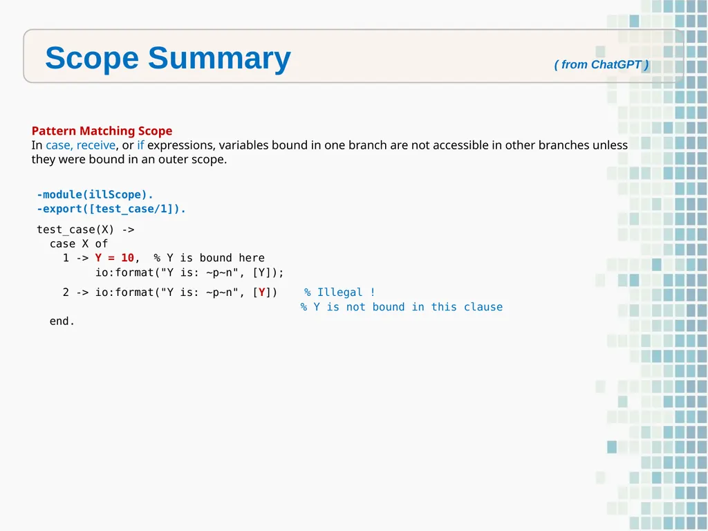
slide59. Scope Summary ( from ChatGPT ) Pattern Matching Scope
In case, receive, or if expressions, variables bound in one branch are not accessible in other branches unless they were bound in an outer scope. -module(illScope).
-export([test_case/1]).
test_case(X) ->
case X of
1 -> Y = 10, % Y is bound here
io:format("Y is: ~p~n", [Y]);
2 -> io:format("Y is: ~p~n", [Y]) % Illegal !
% Y is not bound in this clause
end.<br>
slide60. END<br>
Computer Science Dept
UNC Chapel Hill<br>
slide2. Erlang OTP/BEAM/ERTS<br>
slide3. Erlang A Bit of History Developed by Joe Armstrong et al. at Ericsson, 1986
Proprietary language for programming telephony switches and other communications equipment
Name Erlang is used interchangeably with Erlang/OTP (Open Technology Platform)
Consists of the Erlang runtime system, several ready-to-use components mainly written in Erlang, and a set of design principles for Erlang programs.
Released as free open-source technology in 1998
Erlang/OPT is still maintained at Ericsson
“Erlang” as name a honors the Danish mathematician A.K. Erlang (inventor of queuing theory, and telephone network analysis), as well as a syllabic abbreviation of Ericsson Language<br>
slide4. Erlang Usage Sasa Juric (author) : “Erlang is a development platform for building scalable and reliable systems that constantly provide service with little or no downtime.”
Ericsson’s original need that led to Erlang was telecom systems where properties ike reliability, responsioveness, scalability, and constant availability were imperitive.<br>
slide5. Erlang Usage Tim Bray (Sun Microsystems, 2008: “If somebody came to me and wanted to pay me a lot of money to build a large scale message handling system that really had to be up all the time, could never afford to go down for years at a time, I would unhesitatingly choose Erlang to build it in.”
As of 2014, Erlang was being used in Ericsson nodes, European GPRS networks, 3G and LTE networks worldwide, and by Nortel and T-mobile
WhatsApp is coded in Erlang
Being used in Financial Tech, Gaming, Healthcare, Automotive, IoT and Blockchain platforms, also massively multiple-player online gaming
Used by Vocalink, Goldman Sachs, Nintendo, Samsung, Meta (Facebook)<br>
slide6. Erlang Nature of Erlang Programs The Erlang programming language has
immutable data
pattern matching
functional programming
garbage collection ( and here )
The sequential subset of the Erlang language supports
eager evaluation
single assignment
dynamic typing
A normal Erlang application is built out of hundreds (maybe thousands) of small Erlang processes.<br>
slide7. Erlang BEAM and ERTS BEAM is the virtual machine at the core of the Erlang OTP
BEAM is part of the Erlang Run-Time System ( ERTS ), which compiles Erlang source code into bytecode, which is then run on the BEAM
(wiki) Originally BEAM was short for Bogdan's Erlang Abstract Machine, named after Bogumil "Bogdan" Hausman, who wrote the original version, but the name may also be referred to as Björn's Erlang Abstract Machine, after Björn Gustavsson, who wrote and maintains the current version. Both were done at Ericsson<br>
slide8. Erlang BEAM and ERTS The predecessor of the BEAM was JAM (Joe's Abstract Machine), which was the first virtual machine for the Erlang language and was written by Joe Armstrong.
BEAM bytecode files have the .beam file extension
ERTS is designed for systems with these traits:
Distributed
Fault-tolerant
Soft real-time
Highly available, non-stop applications
Hot swapping, where code can be changed without stopping a system<br>
slide9. Erlang Processes Erlang applications are built of very lightweight processes in the ERTS.
Erlang processes can be seen as "living" objects, with data encapsulation and message passing, but capable of changing behavior during runtime.
ERTS provides
strict process isolation between Erlang processes
transparent communication between processes on different Erlang nodes (on different hosts).
Armstrong in 2013 said “ If Java is 'write once, run anywhere', then Erlang is 'write once, run forever'. ”<br>
slide10. Processes ( from erlang.org ) In Erlang, each thread of execution is called a process.
Aside: the term "process" is usually used when the threads of execution share no data with each other and the term "thread" when they share data in some way; threads of execution in Erlang share no data, so are termed processes
Erlang is designed for massive concurrency
Erlang processes are lightweight (grow and shrink dynamically) with small memory footprint, fast to create and terminate, and the scheduling overhead is low<br>
slide11. Processes ( from erlang.org ) Communication in Erlang is conceptually performed using asynchronous signaling.
All different executing entities, such as processes and ports, communicate through asynchronous signals.
The most commonly used signal is a message, but other common signals are exit, link, unlink, monitor, and demonitor signals.
So, the basic unit of concurrency in Erlang is a process -- a lightweight thread of execution that runs independently and communicates with other processes through message passing<br>
slide12. Processes ( from erlang.org ) Processes are created with the spawn function, which takes a function as an argument and returns a process identifier (pid).
An Erlang “program” is a call to an initial function (in a module); that function may spawn other processes… which may spawn more, etc.
Erlang processes operate in (memory) isolation from each other, and are scheduled by Erlang's Virtual Machine (VM).
The creation time of process is very low, the memory footprint of a just spawned process is very small, and a single Erlang VM can have millions of processes running.
The default max number of alive processes is by default 32,768. This limit can be raised up to 268,435,456 processes at startup.<br>
slide13. Erlang Principles of Erlang Processes Everything is a process.
Processes are strongly isolated.
Process creation and destruction is a lightweight operation.
Message passing is the only way for processes to interact.
Processes have unique names.
If you know the name of a process you can send it a message.
Processes share no resources.
Error handling is non-local.
Processes do what they are supposed to do or fail.<br>
slide14. Erlang “Let it crash” or “Let it fail” Erlang supports a "Let it fail" coding style
Has a mechanism that makes it easy for external processes to monitor for crashes (or hardware failures). This is In preference to an in-process mechanism like exception handling used in many other PLs
Crashes are reported like other messages (the only way processes can communicate with each other). Subprocesses can be spawned cheaply
So prefer a process be completely restarted rather than trying to recover from a failure
This philosophy results in less code devoted to defensive programming where error-handling code is highly contextual and specific<br>
slide15. Let it fail …. means “Let it crash” or “Let it fail” Design philosophy: design systems expecting that failure will happen; build a supervisor structure to monitor executions, detect failures, and quickly restart failed processes
Error detection via supervisor infrastructure
Fail fast, then recover
Isolation of failures<br>
slide16. Now… How to Erlang Based on an Interpreted Shell Basic Shell, Runtime: https://www.erlang.org/downloads
Some IDEs will allow you to build and run Erlang programs
Also here is a page that lets you run it on the web:
https://onecompiler.com/erlang
Interactive tutorial: https://tryerlang.org/<br>
slide17. Syntax Quick Summary Variables
are sequences of characters as in most PLs, but must begin with an uppercase letter. A variable may be given a value of some basic datatype. Variables are single assignment; once given a value, a variable cannot have its value changed. Hence, a “variable” is not variable .
Atoms
are sequences of characters like variables, but must begin with a lowercase letter. It can be enclosed in single quotes when needed. The value of an atom is its name. It is just a symbol. It is a basic datatype.
Functions
named (usually) sequences of expressions to be evaluated. Erlang is a functional language, so function execution (expression evaluation) is the primary means of computation being carried out.
Modules
The primary mechanism for organizing Erlang code. Modules contain function definitions.<br>
slide18. Syntax Quick Summary Basic Data Types
Atom, Integer, Float, Binary, Pid, Port, Fun
Structured Types
List: dynamic mixed collection, using brackets: [1,”2”,three]
Tuple: fixed-length mixed collection, using braces: { “foo”, abc, 123}
Pattern Matching
Used in function parameter binding, many other places
[ H | R ] = [6,7,18,90,2001]. %% H gets 6, R gets [7,18,90,2001]
Guards
Used to partially define function clauses, other selections
factorial(0) -> 1;
factorial(N) when N > 0 -> N * factorial(N - 1).<br>
slide19. Syntax Quick Summary Conditional Flow Control
If/Then : alternative to guards
Case : pattern matching in blocks
Receive : handling messages in processes selectively
Recursion
Functional language way of “looping”, as well as manipulating recursively defined structures like lists
Processes
Basic unit of execution, as well as concurrency
Lightweight, communicate via message passing
Several common important process patterns
-- like monitor, supervisor, server<br>
slide20. Erlang Shell Using the erlang shell, command line Runs from the erlang icon after installation
To exit, type q(). at the command line prompt
Alternately, ctrl + G and then in job control mode, type q (no ending .) 1> pwd().
c:/Program Files/erl-24.1/usr
2> 5.
5
3> foo.
foo
4> Foo.
* 1:1: variable ‘Foo’ is unbound
5> q(). and the shell goes poof
Or
5> ctrl+G
User switch command
--> q
and the shell goes poof, all definitions and binding gone<br>
slide21. Erlang Data Basic data types (8 of them) Integer
Integers are written as sequences of decimal digits, for example, 12, 12375 and -23427 are integers. Integer arithmetic is exact and only limited by available memory on the machine.
Atoms
Atoms are used within a program to denote distinguished values. They are written as strings of consecutive alphanumeric characters, the first character being lowercase. They are simply symbols with no “value”. Atoms are never garbage collected.
Floats
Floating point numbers use the IEEE 754 64-bit representation
References
References are globally unique symbols whose only property is that they can be compared for equality. They are created by evaluating the Erlang primitive make_ref().<br>
slide22. Erlang Data Basic data types (8 of them) Binaries
A binary is a sequence of bytes. Binaries provide a space-efficient way of storing binary data. Erlang primitives exist for composing and decomposing binaries and for efficient input/output of binaries.
Pids
Pid is short for process identifier; a Pid is created by the Erlang primitive spawn(...) . Pids are references to Erlang processes.
Ports
Ports are used to communicate with the external world. Ports are created with the built-in function open_port. Messages can be sent to and received from ports, but these messages must obey the so-called "port protocol."
Funs
Funs are function closures. Funs are created by expressions of the form: fun(...) -> ... end.<br>
slide23. Erlang Data Compound types (3 of them) Tuples
Tuples are containers for a fixed number of Erlang data values. Syntax {D1,D2,...,Dn} denotes a tuple whose arguments are D1,D2,...Dn. The arguments can be primitive data types or compound data types. Any element of a tuple is accessed in constant time.
Lists
Lists are containers for a variable number of Erlang data values. The syntax [Dh|Dt] denotes a list whose first element (head) is Dh, and whose remaining elements (tail) are the list Dt. The syntax [] denotes an empty list. The syntax [D1,D2,..,Dn] is short for [D1|[D2|..|[Dn|[]]]]. The first element of a list can be accessed in constant time.
Maps
Maps contain a variable number of key-value associations. The syntax is #{ Key1=>Value1, ..., KeyN=>ValueN } .<br>
slide24. Examples: Lists Workhorse Data Structure of Functional Languages [1,2,3,5,8,13].
Fabs = [1,2,3,5,8,13].
hd(Fabs). % 1
tl(Fabs). % [2,3,5,8,13]
[A | Rest] = Fabs. % use patterns bind parts of list to vars
A. % 1
Rest. % [2,3,5,8,13]
L1 = [2,3.14159, “goheels”]. % heterogeneous, arbitrary length
L2 = [ “gamma”, [ 2,3,5.5], L1, [L1, “delta”], hd(tl(Fabs)) ].
% structure is fine
lists:map(fun(X) -> 2*X end, Fabs). % [2,4,6,10,16,26]
Double = fun(X) -> 2*X end.
lists:map(Double, [14, -10, 5, 101]). % [28, -20, 10, 202]<br>
slide25. Examples: Lists Remember string is a list of char representations? [75,76,77]. % print “KLM” but it’s a list of ints
hd(“heels”). % 104 not “h”
tl(“heels”) % this says “eels” though
hd(tl(“heels”)). % 101
UNC = “go_heels”.
[ U | NC ] = UNC. % use patterns, bind parts of list to vars
U. % 103
NC. % “o_heels”<br>
slide26. Examples: Tuples Heterogeneous Fixed-size collection Lists are arbitrary length (you can grow them dynamically)
Tuples are fixed length… fields cannot be added once a tuple is made
Elements in fields of a tuple can be heterogeneous { won, 2, “three” }.
Tup = { won, 2, “three” }.
element(2,Tup). % 2
element(1,Tup). % won
Origin = {0,0}.
{X,Y} = Origin.
X. % 0
Y.
element(4,{ one, 2, “tree”, fore, “V”, ‘VI’, VII }). % fore ?
% unless variable VII is not defined ‘Single quotes’ for atom that begins with uppercase<br>
slide27. Examples: Maps Like the Common ADT MAP A map is a tuple of key, value pairs
Lookup, remove, get, put, etc. common map operations are available MM = #{name=>"john",age=>34,year=>3,height=>5.85}.
map_get(name,MM). % “john”
maps:put(rank, "assistant",MM). % maps:get(_,_)
map_get(rank,MM). % does what?
Lst1 = [{"a",1},{"b",2},{"c",3}].
Map1 = maps:from_list(Lst1).
io:fwrite("~p~n",[maps:put("d",4,Map1)]).
% #{"a" => 1,"b" => 2,"c" => 3,"d" => 4} -module(helloworld). -export([start/0]). start() -> Lst1 = [{"a",1},{"b",2},{"c",3}], Map1 = maps:from_list(Lst1), io:fwrite("~p~n",[maps:put("d",4,Map1)]). #{"a" => 1,"b" => 2,"c" => 3,"d" => 4}<br>
slide28. Examples: Strings Strings are not a data type “Strange”. % shorthand for a list [ $S,$t,$r,$a,$n,$g,$e ]
% where $c is the ascii or unicode for character c
Mood = “mellow”.
Mood. % symbols that start with upper case are
% variables and can be bound (once)
[49,50,51,65].
% look what the shell replies
% strange, no?
So strings as “quoted character sequences” are just syntactic shorthand for the internal representation, a list of ascii numbers representing the character
One of the things about Erlang most agree needs cleaning up<br>
slide29. 23> "go unc".
"go unc“
24> hd("go unc").
103
25> tl("go unc").
“o unc”
26> hd(tl("go unc")).
111
27> "o".
"o"
28> hd ("o").
111
29> hd([2]).
2
30> hd("2").
50
31> hd(2).
** exception error: bad argument
in function hd/1
*** argument 1: not a nonempty list Using the erlang shell, command line Fun Erlang Stuff<br>
slide30. io:fwrite(“Hello, World!”).
io:fwrite(“Name: ~s~n”, [“Dave”]).
io:fwrite(“~s ~p ~n”, [“Age: “, 45]).
io:format(“~s ~p ~n”, [“Age: “, 45]).
% io:fwrite is a synonym for io:format Output Formatted<br>
slide31. Module Format Source Code and Compiled Code Erlang code is divided into modules.
A module consists of a sequence of attributes and function declarations, (and a few other things… like records, type specs, etc.) each terminated by period (.) -module(modex). % module attribute, predefined
-export([fact/1]). % module attribute, predefined
-coder(stotts). % user defined attribute
% function declaration (by clauses)
fact(N) when N>0 -> N * fact(N-1);
fact(0) -> 1. This source text must be in a file named “ modex.erl “
Compiler (in shell) compiles it into a file “ modex.beam “ which contains bytecode for the BEAM VM<br>
slide32. Compile and Execute Using the erlang shell, command line Find the erlang code examples (a directory of modules)
Look for “modex.erl” a text file containing an erlang module 1> pwd().
c:/Users/stotts/Desktop
2> cd(“erlCode”).
c:/Users/stotts/Desktop/erlCode
3> ls().
joeCode links.erl lp.erl
modex.erl monitors.erl name_server.erl
4> c(“modex”).
{ok,modex}
5> ls().
joeCode links.erl lp.erl
modex.beam modex.erl monitors.erl
6> modex:fact(25).
15511210043330985984000000
7> modex:fact(41).
33452526613163807108170062053440751665152000000000<br>
slide33. Function Declaration Anonymous Functions A function can be created as an anonymous value
Once created, this value can be used in another expression (such as passed as a parameter to another function call)
Can also be bound to a variable (i.e., “named”) Negate = fun(I) -> -I end .
#Fun<erl_eval.6.13229925>
17> Negate(1).
-1
18> Negate(-10).
10
Numbers = [1, 2, 3, 4].
[1,2,3,4]
2> lists:foreach( fun(Nums) -> io:format("num: ~p~n", [Nums]) end , Numbers ). Examples in the shell:<br>
slide34. Defining Functions in the Shell Functions usually defined in modules, but it is possible in shell First, define an anonymous function, then bind it to a variable as its name >> T5 = fun(N) -> N*5 end.
>> T5(41).
205
>> Foo = fun (0, _) -> 0 ; %% defined via alternatives
(1, N) -> N ;
(N1, N2) -> N1*N2
end.
>> Foo(0,212).
0
>> Foo(12,31).
372<br>
slide35. Defining Functions in the Shell What about recursive functions? %% this wont work
>> SumL = fun ([], []) -> [];
([H1 | T1], [H2 | T2]) -> [H1 + H2 | SumL(F, T1, T2)]
end. The variable SumL is not defined here
when we use it in a clause defining SumL<br>
slide36. Defining Functions in the Shell What about recursive functions? %% this will
>> SumL = fun
(F, [], []) -> [];
(F, [H1 | T1], [H2 | T2]) -> [H1 + H2 | F (F, T1, T2)]
end.
%% here the “recursive” func is passed in as a
%% parameter F, and called in the second clause
>> SumL(SumL, [2,4,6], [1,3,5]).
[3,7,11] %% this wont work
>> SumL = fun ([], []) -> [];
([H1 | T1], [H2 | T2]) -> [H1 + H2 | SumL(F, T1, T2)]
end.<br>
slide37. Function Declaration A function declaration is a sequence of function clauses separated by semicolons, and terminated by period (.)
A function clause consists of a clause head and a clause body, separated by ->
A clause head consists of the function name, an argument list, and an optional guard sequence beginning with the keyword when: -module(modex). % module attribute, predefined
-export([fact/1]). % module attribute, predefined
% function declaration (by clauses)
fact(N) when N>0 -> N * fact(N-1);
fact(0) -> 1. Function name is an atom (so starts lowercase).
Binding a variable (starts upper case start) to an anonymous function, is different from naming a function in a module. You cannot export the variable in a module like you can export a named function.
Number of arguments to the function is the arity of the function. Here, function “fact” is denoted fact/1 in the export attribute of a module to show it has arity 1
Fully qualified name of this function is: modex:fact/1
To call the function do this: modex:fact(25). Functions are usually defined in modules<br>
slide38. -module(my_mod).
-export([my_func/1]).
my_func(Value) -> % a function name, an atom my_func
% Binding an anonymous function to a variable
Square = fun(X) -> X * X end, % anon function bound to variable Square
% Using the anonymous function inside the named function
Result = Square(Value),
Result. Named Function vs. Var Binding Function name my_func is an atom (so starts lowercase).
Named function can be exported (and so used outside this module
Bound anon function cannot be exported, and so must be
-- defined inside a named function
-- must be used in this module… in fact, inside the containing defined function This module uses both methods<br>
slide39. Tail Recursion Tail recursion allows “infinite loops” in a functional PL >> Review of (Java) stack frames, runtime stack, recursion Tail recursion is
-- recursion ( !! )
-- recursive call is last thing done in the function body
-- means no computation is needed in a function invocation when the
recursive call returns with no computation needed after recursive call returns, then the state saved in the stack frame is not needed
variable values computed before the recursive call do not need to be preserved for use after the return
-- So, the recursive call can “reuse” the stack frame for the invoking call
-- So, tail-recursive functions use ONE stack frame
-- So, tail-recursion can continue indefinitely without blowing out the runtime stack<br>
slide40. (Sequential) Erlang Examples Fibonacci (tail recursive) -module(series).
-export([fib/1]).
fib(0) -> 0;
fib(N) when N < 0 -> err_neg_val;
fib(N) when N < 3 -> 1;
fib(N) -> fib_int(N, 0, 1).
fib_int(1, _, B) -> B; % this is not exported
fib_int(N, A, B) -> fib_int(N-1, B, A+B).<br>
slide41. Erlang Examples Fibonacci (tail recursive) annotated %% -- Header Information -----------------------------------------
%% The module declaration must match the file name "series.erl"
-module(series).
%% The export statement contains a list of all functions that form
%% the module's public API. Here this module exposes a single
%% function called fib that takes 1 argument (i.e. has arity of 1)
%% The general syntax for -export is a list containing the name and
%% arity of each public function
-export([fib/1]).<br>
slide42. Erlang Examples % Public API ============================================== %% Handle cases in which fib/1 receives specific values
%% The order in which these partial function cases appear is vital
%% If fib/1 is passed precisely the integer 0, then return 0
fib(0) -> 0;
%% If fib/1 receives a negative number, then return atom err_neg_val
%% Normally, defensive coding is discouraged due to Erlang's 'Let
%% it Crash' philosophy; however, in this case we do explicitly
%% prevent a situation that will crash Erlang's runtime engine
fib(N) when N < 0 -> err_neg_val;
%% If fib/1 is passed an integer less than 3, then return 1
%% The preceding two partial functions handle all cases where N<1
%% so next we handle cases where N = 1 or N = 2
fib(N) when N < 3 -> 1;
%% For all other values, call private function fib_int/3
fib(N) -> fib_int(N, 0, 1).<br>
slide43. Erlang Examples % Private API ================================================= %% If fib_int/3 gets a 1 as its first arg, we're done,
%% so return the value in arg B. Since not interested
%% in the value of the second arg, we denote this using
%% _ indicating a "don't care" value
fib_int(1, _, B) -> B;
%% For all other arg combos, recursively call fib_int/3
%% where each call does the following:
%% - decrement counter N
%% - Take the previous fibonacci value in arg B and
%% pass it as arg A
%% - Calc the value of the current fibonacci number
%% and pass it as arg B
fib_int(N, A, B) -> fib_int(N-1, B, A+B).<br>
slide44. Recursion using Stack Frames -module(rec).
-export([len/1]).
len([]) -> 0;
len([_|T]) -> 1 + len(T). Let’s compute length of a list English:
A list is length 0 when empty,
and 1 more that the length of the rest of the list when not empty. len([1,2,3,4]) = len([1 | [2,3,4])
= 1 + len([2 | [3,4]])
= 1 + 1 + len([3 | [4]])
= 1 + 1 + 1 + len([4 | []])
= 1 + 1 + 1 + 1 + len([])
= 1 + 1 + 1 + 1 + 0
= 1 + 1 + 1 + 1
= 1 + 1 + 2
= 1 + 3
= 4 Behavior on run-time stack during recursive calls Each is a stack frame… storage Not tail recursive… there is
work to do in each invocation
after the recursion returns<br>
slide45. Tail-Recursion vs. Non -module(factorial).
-export([fact/1]).
% Non-tail recursive factorial function
fact(0) -> 1;
fact(N) when N > 0 -> N * fact(N - 1). First, recursive factorial that is NOT tail recursive Erlang code public static int factorial(int n) {
if (n == 0) return 1; // Base case
} else { return n * factorial(n-1); } // Recursive call
}
public static int factorial(int n) {
if (n == 0) return 1; // Base case
} else { temp = factorial(n-1); // recursive call, put result in stack frame
return n * temp; } // more work after, using state from stack frame
} Java code (shows “extra work” after the call)<br>
slide46. Erlang Tail Recursion -module(rec).
-export([fac/1]).
fac(N) -> tail_fac(N,1).
tail_fac(0,Acc) -> Acc;
tail_fac(N,Acc) when N > 0 -> tail_fac(N-1,N*Acc). Let’s eliminate the “state” stored in all those stack frames Pass extra parameters to the recursive call… accumulate as your go, so to speak
We saw this before in recursive factorial So do this with len… add an accumulator parameter -module(rec).
-export([len/1]).
len(L) -> tail_len(L,0).
tail_len([], Acc) -> Acc;
tail_len([_|T], Acc) -> tail_len(T,Acc+1).<br>
slide47. Erlang Tail Recursion -module(rec).
-export([for/2, inf/0]).
for(L, 0) -> L; % index runs out before list
for([], I) -> I; % list runs out before index
for(L, I) ->
io:fwrite("~p: ~p ~n", [I, hd(L)]), % “loop body”
for( tl(L), I-1). % tail recursion, do “loop body” over again
inf() ->
io:fwrite("some 'loop body' action \n"),
timer:sleep(3000),
inf(). % tail recursion More Examples and Uses Equivalent of looping … for loop shown here
Process “cycle” (infinite)<br>
slide48. Erlang Examples Quicksort %% quicksort a list of elements (as long as ‘<‘ is defined for the type)
-module(quick). % This is the file ‘quick.erl'
-export([sort/1]). % fun 'sort' with 1 parm (no type, no name)
sort( [] ) -> []; % If empty list, return empty (nothing to sort)
sort( [Pivot|Rest] ) ->
% Compose recursively a list with 'Front' being all elements
% that should be before 'Pivot‘,
% then 'Pivot‘,
% then 'Back' being all elements that should be after 'Pivot’
sort( [Front || Front <- Rest, Front < Pivot] )
++ [Pivot]
++ sort( [Back || Back <- Rest, Back >= Pivot] ) .<br>
slide49. Erlang Examples Quicksort list of lists % This version of quicksort sorts a list of lists
% it puts the lists in order of list length, shortest list first
% it uses the ‘length’ function on lists as the ordering metric
-module(qquick).
% Export ‘sort' with 1 parameter (don't care about the type and name)
-export([sort/1]). % sort/2 is private… not exported … here it’s a helper function
sort(Lists) -> % call sort/2 and send
sort(Lists, fun(A,B) -> length(A) < length(B) end). % anonymous function as 2nd parameter
sort( [], _ )-> []; % If list is empty, return empty (ignore 2nd param)
sort( [Pivot|Rest], Smaller ) ->
% Partition list with 'Smaller' elements in front of 'Pivot' and
% not-'Smaller' elements after 'Pivot' and sort the sublists.
sort([X || X <- Rest, Smaller(X,Pivot)], Smaller)
++ [Pivot]
++ sort([Y || Y <- Rest, not(Smaller(Y, Pivot))], Smaller).<br>
slide50. Control Structures Conditionals: case Animal = "dog".
case Animal of % what if Animal = “fish” ?
"dog" -> under;
"cat" -> thunder
end.
case Animal of
"lion" -> food;
_ -> something_else % ‘default’ case
end.
% what does this do?
case Animal of
'dog' -> under;
'cat' -> thunder
end.<br>
slide51. Control Structures Conditionals: if X = 0.
if
X > 0 -> positive;
X < 0 -> negative
end.
** exception error: no true branch found when evaluating an if expression
if
X > 0 -> positive; % then
X < 0 -> negative; % elseif
true -> zero % ‘otherwise’ clause, matches anything
end.
if
Count > Flag -> someThenOperation();
true -> someElseOperation()
% Count <= Flag -> someElseOperation()
end. Based on guards which is Erlang-speak for Boolean conditions
X > 0 -> positive<br>
slide52. Erlang BIF’s -module(examples).
-export([start/0]).
start() ->
io:fwrite( "~p~n", [ tuple_to_list({1,2,3}) ] ),
io:fwrite( "~p~n", [ time() ] ),
io:fwrite( “~p~n”, [ now() ] ), % { megasecs, secs, microsecs }
% since Jan 1 1970 Built In Functions BIFs are functions that are built into Erlang.
Provided to do tasks that are impossible to program in the rest of Erlang.
For example, it’s we cant convert a list into a tuple
We can’t find the current time and date, so we call a BIF.<br>
slide53. More BIF’s -module(examples).
-export([start/0]).
start() ->
io:fwrite( "~p~n", [ element( 2, {one,“two”,3.3,delta} ) ] ),
% shows the built-in “process dictionary”
% nice note pad
% not a map but a list of 2-tuples
io:fwrite( "~p~n", [ put( pi, 3,14159) ] ),
io:fwrite( "~p~n", [ get( pi ) ] ),
io:fwrite( "~p~n", [ get( ) ] ),
io:fwrite( "~p~n", [ erase( pi ) ] ),
io:fwrite( "~p~n", [ erase( ) ] ).
% also bunch of these
% is_atom(T), is_binary(T), is_function(T), is_float(T)
% is_integer(T), is_number(T), is_list(T), is_record(T), etc.<br>
slide54. Scope in Erlang Variables in a clause exist from point of first binding to the last textual reference to that variable within the clause.
Binding of a variable can only happen in a pattern matching operation (like “=“).
Can think of the pattern match as “producing” the variable and binding. Example:
f(X) -> % 1 var X is defined, and is bound when f is called
% g(Y), % here would get Y unbound error
Y = g(X), % 2 X has its value used
% Y is defined (its first occurrence)
h(Y,X), % 3 X and Y values used
p(Y). % 4 Y used No variables (names bound to values) may be exported from a fun.
All variables in head of a function are “fresh” (shell example)
Any variable defined before the fun may be used in guards, or fun calls within a fun<br>
slide55. Scope in Erlang %% shell example
%%
%% L = [12,123,1234,23,234,2345].
%%
%% NN = fun(L) -> -L end.
%%
%% NN(5).
%%
%% NNN = fun(X) -> io:fwrite("~p ~n", [ hd(L) ]), X*2 end.
%%
%% NNN(5).
%% No variables (names bound to values) may be exported from a fun.
All variables in head of a function are “fresh” (shell example)
Any variable defined before the fun may be used in guards, or fun calls within a fun<br>
slide56. Scope in Erlang % tests
-module(hw).
-export([ff/1, fff/1]).
p(H) -> io:fwrite("~p~n", [H]).
h(A,B) -> io:fwrite("~p ~p ~n", [A,B]).
g(C) -> io:fwrite("~p~n", [-C]).
ff(X) ->
%g(Y),
Y = g(X),
h(Y,X),
p(Y).
fff(C) -> io:write("~p ~n", [ Y ] ), C.
% ^^ Y is unbound here No variables (names bound to values) may be exported from a fun.
All variables in head of a function are “fresh” (shell example)
Any variable defined before the fun may be used in guards, or fun calls within a fun<br>
slide57. Scope in Erlang In if, case, and receive structures, variables created are exported to the code after the selection structure… with some restrictions f(X) ->
case g(X) of
true -> A = h(X);
false -> A = k(X)
end,
. . .
% variable A is available to be used here
% and after in function f Restriction: different selection branches must define the same set of variables, (unless the missing vars are not referenced after the selection structure) f(X) ->
case g(X) of
true -> A=h(X), B=A+7;
false -> B=6
end,
h(A). % illegal f(X) ->
case g(X) of
true -> A=h(X), B=A+7;
false -> B=6
end,
h(B). % legal<br>
slide58. Scope Summary ( from ChatGPT ) Single Assignment
Variables are immutable once assigned and cannot be re-bound within the same scope.
Sequential Scope
Variables are accessible only after they are bound.
Nested Scope
Inner expressions (e.g., case statements) cannot leak variables to outer expressions.
No Global Variables
Erlang does not have global variables; everything is local to the function, module, or process.
Process Isolation
Each process has its own scope, and variables cannot be shared between processes.
Function Scope
Variables defined in a function are local to that function and can't be accessed from outside it.
List Comprehensions and Anonymous Functions
Variables defined within these constructs are local. Outer scope variables are accessible inside, but not vice versa.
Module Scope
Erlang has no global variables, and state is passed explicitly between functions, promoting functional purity. Functions do not share variables unless passed as arguments.<br>
slide59. Scope Summary ( from ChatGPT ) Pattern Matching Scope
In case, receive, or if expressions, variables bound in one branch are not accessible in other branches unless they were bound in an outer scope. -module(illScope).
-export([test_case/1]).
test_case(X) ->
case X of
1 -> Y = 10, % Y is bound here
io:format("Y is: ~p~n", [Y]);
2 -> io:format("Y is: ~p~n", [Y]) % Illegal !
% Y is not bound in this clause
end.<br>
slide60. END<br>