
Portfolio Management Prof Anil K kothari 1































Description: Portfolio Management Prof Anil K kothari 1 Systematic Risk vs. Unsystematic Risk Systematic Risk These are market risksthat is, general perils of investingthat cannot be diversified away. Interest rates, recessions, and wars are
Related Topics
Download Presentation
"Portfolio Management Prof Anil K kothari 1" is the property of its rightful owner. Permission is granted to download and print the materials on this website for personal, non-commercial use only, and to display it on your personal computer provided you do not modify the materials and that you retain all copyright notices contained in the materials. By downloading content from our website, you accept the terms of this agreement.
Presentation Transcript
slide1. Portfolio Management Prof Anil K kothari 1<br>
slide2. Systematic Risk vs. Unsystematic Risk Systematic Risk – These are market risks—that is, general perils of investing—that cannot be diversified away.
Interest rates, recessions, and wars are examples of systematic risks.
Unsystematic Risk – Also known as "specific risk," this risk relates to individual stocks. In more technical terms, it represents the
component of a stock's return that is not correlated with general market moves. Modern portfolio theory shows that specific risk can be removed or at least mitigated through diversification of a portfolio. The trouble is that diversification still does not solve the problem of systematic risk; even a portfolio holding all the shares in the stock market can't eliminate that risk. Therefore, when calculating a deserved return, systematic risk is what most plagues investors. The capital asset pricing model was developed by the financial economist (and later, Nobel laureate in economics) William Sharpe, set out in his 1970 book Portfolio Theory and Capital Markets. His model starts with the idea that individual investment contains two types of risk: 2<br>
slide3. 3<br>
slide4. The capital asset pricing model (CAPM) is the equation that describes the relationship between the expected return of a given security and systematic risk as measured by its beta coefficient. Besides risk the model considers the effect of risk-free interest rates and expected market return.
Assumptions
Basic assumptions of the CAPM model are as follows.
Markets are ideal—no transaction fees, taxes, inflation, or short selling restrictions.
All investors are averse to risk.
Markets are highly efficient. All investors have equal access to all available information.
All investors can borrow and lend unlimited amounts under a risk-free rate.
Beta coefficient is the only measure of risk.
All assets are absolutely liquid and infinitely divided.
The amount of available assets is fixed during a given period of time.
Markets are in equilibrium. All investors are price takers, not price makers.
Return of all available assets is subject to normal distribution function. 4<br>
slide5. 5<br>
slide6. The Capital Asset Pricing Model (CAPM) measures the risk of a security in relation to the portfolio. It considers the required rate of return of a security in the light of its contribution to total portfolio risk. The CAPM holds that only undiversifiable risk is relevant to the determination of expected return on any asset.
Even though the CAPM is competent to examine the risk and return of any capital asset such as individual security, an investment project or a portfolio asset 6<br>
slide7. Assumptions of Capital Asset Pricing Model
The CAPM is based on the following assumptions.
1. Risk-averse investors
The investors are basically risk averse and diversification is necessary to reduce their risks.
2. Maximising the utility of terminal wealth
An investor aims at maximizing the utility of his wealth rather than the wealth or return. The term ‘Utility’ describes the differences in individual preferences. Each increment of wealth is enjoyed less than the last as each increment is less important in satisfying the basic needs of the individual. Thus, the diminishing marginal utility is most applicable to wealth.
There are also other forms of utility functions. Some investors showing a preference for larger risks are those who have increasing marginal utility for wealth. In such cases, each increase in wealth prompts the individual to acquire more wealth. For a risk-neutral investor, each increment in wealth is equally attractive. In other words, each increment would have the same utility for him. 7<br>
slide8. 3. Choice on the basis of risk and return:
Investors make investment decisions on the basis of risk and return. Risk and return are measured by the variance and the mean of the portfolio returns. CAPM assumes that the rational investors put away their diversifiable risk, namely, unsystematic risk. But only the systematic risk remains which varies with the Beta of the security.
Some investors use the beta only to measure the risk while other investors use both beta and variance of returns as the sources of reward. As individuals have varying perceptions towards risk and reward, CAPM gives a series of efficient frontlines. 4. Similar expectations of risk and return
All investors have similar expectations of risk and return. In other words, all investors’ estimates of risk and return are the same. When the expectations of the investors differ, the estimates of mean and variance lead to different forecasts.
As a result, there will be innumerable efficient frontiers and the efficient portfolio of each will be different from that of the others. Varying preferences also imply that the price of an asset will be different for different investors. 5. Identical time horizon
The CAPM is based on the assumption that all investors have identical time horizon. The core of this assumption is that investors buy all the assets in their portfolios at one point of time and sell them at some undefined but common point in future. This assumption further implies that investors form portfolios to achieve wealth at a single common terminal rate. 8<br>
slide9. 6. Free access to all available information
One of the important assumptions of the CAPM is that investors have free access to all the available information at no cost. Supposing some investors alone are able to have access to special information which is not readily available to all, then the markets would not be regarded efficient. In other words, if the available information has not reached all, it will be difficult to draw a common efficient frontier line. 7. There is risk-free asset and there is no restriction on borrowing and lending at the risk free rate
This is a very important assumption of the CAPM. The risk free asset is essential to simplify the complex pairwise covariance of Markowitz’s theory. The risk free asset makes the curved efficient frontier of MPT to the linear efficient frontier of the CAPM simple.
As a result, the investors will not concentrate on the characteristics of individual assets. By adding a portion of risk-free assets to the portfolio and borrowing the additional funds needed at a risk free rate, the risk is either decreased or increased. 8. There are no taxes and transaction costs
According to Roll, there must be either a risk free asset or a portfolio of short sold securities. Then only the capital Market Line (CML) will be straight. When there are no risk free assets, the investor could not create a proxy risk free asset. As a result, the capital market line would not be linear and the direct linear relationship between risk and return would not exist. 9. Total availability of assets is fixed and assets are marketable and divisible
This assumption holds the view that the total asset quantity is fixed and all assets are marketable. 9<br>
slide10. Formula
The CAPM model allows you to assess the expected return of a given security using the following formula:
E(Ri) = RF + βi × (E(RM) - RF)
where E(Ri) is an expected return of a security, RF is a risk-free rate, βi is the beta coefficient of a security, and E(RM) is an expected Market risk premium (RPM) can be calculated as follows.
RPM) = E(RM) - RF
The risk premium of a given security (RPi) can be assessed as follows:RPi) = βi × (E(RM) - RF)
Example
Let’s assume an investor is thinking of buying one of three stocks: Stock A with a beta of 0.85, Stock B with a beta of 1.25, and Stock C with a beta of 1.65. If the risk-free rate is 4.50% and the expected market return is 12.35%, the expected return of each security can be assessed under CAPM. E(RA) = 4.50 + 0.85 × (12.35 - 4.50) = 11.17%
E(RB) = 4.50 + 0.85 × (12.35 - 4.50) = 14.31%
E(RC) = 4.50 + 0.85 × (12.35 - 4.50) = 17.45%
Thus, a relationship exists between risk and the expected return of a security. So, the higher the beta, the higher the expected return and vice versa. 10<br>
slide11. CAPM's starting point is the risk-free rate–typically a 10-year government bond yield. A premium is added, one that equity investors demand as compensation for the extra risk they accrue. This equity market premium consists of the expected return from the market as a whole less the risk-free rate of return. The equity risk premium is multiplied by a coefficient that Sharpe called "beta." Beta's Role in CAPM
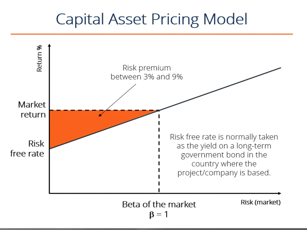
According to CAPM, beta is the only relevant measure of a stock's risk. It measures a stock's relative volatility–that is, it shows how much the price of a particular stock jumps up and down compared with how much the entire stock market jumps up and down. If a share price moves exactly in line with the market, then the stock's beta is 1. A stock with a beta of 1.5 would rise by 15% if the market rose by 10% and fall by 15% if the market fell by 10%. Beta, compared with the equity risk premium, shows the amount of compensation equity investors need for taking on additional risk. If the stock's beta is 2.0, the risk-free rate is 3%, and the market rate of return is 7%, the market's excess return is 4% (7% - 3%). Accordingly, the stock's excess return is 8% (2 x 4%, multiplying market return by the beta), and the stock's total required return is 11% (8% + 3%, the stock's excess return plus the risk-free rate). What the beta calculation shows is that a riskier investment should earn a premium over the risk-free rate. The amount over the risk-free rate is calculated by the equity market premium multiplied by its beta. In other words, it is possible, by knowing the individual parts of the CAPM, to gauge whether or not the current price of a stock is consistent with its likely return. 11<br>
slide12. 12<br>
slide13. Portfolio diversification
CAPM deals with the risks and returns on financial securities and defines them precisely, if arbitrarily. The rate of return an investor receives from buying a common stock and holding it for a given period of time is equal to the cash dividends received plus the capital gain (or minus the capital loss) during the holding period divided by the purchase price of the security.
Although investors may expect a particular return when they buy a particular stock, they may be disappointed or pleasantly surprised, because fluctuations in stock prices result in fluctuating returns. Therefore common stocks are considered risky securities. (In contrast, because the returns on some securities, such as Treasury bills, do not differ from their expected returns, they are considered riskless securities.) Financial theory defines risk as the possibility that actual returns will deviate from expected returns, and the degree of potential fluctuation determines the degree of risk.
An underpinning of CAPM is the observation that risky stocks can be combined so that the combination (the portfolio) is less risky than any of its components. Although such diversification is a familiar notion, it may be worthwhile to review the manner in which diversification reduces risk. 13<br>
slide14. The security market line
The culmination of the sequence of conceptual building blocks is CAPM’s risk/expected return relationship. This fundamental result follows from the proposition that only systematic risk, measured by beta (β), matters. Securities are priced such that:
Rs = Rf + risk premium
Rs = Rf + βs (Rm – Rf)
Where: Rs = the stock’s expected return (and the company’s cost of equity capital).
Rf = the risk-free rate.
Rm = the expected return on the stock market as a whole.
β s = the stock’s beta.
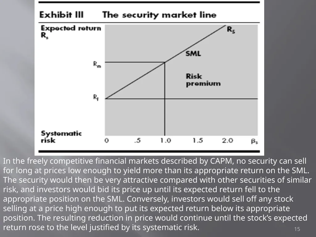
This risk/expected return relationship is called the security market line (SML). I have illustrated it graphically in Exhibit III. As I indicated before, the expected return on a security generally equals the risk-free rate plus a risk premium. In CAPM the risk premium is measured as beta times the expected return on the market minus the risk-free rate. The risk premium of a security is a function of the risk premium on the market, Rm – Rf, and varies directly with the level of beta. (No measure of unsystematic risk appears in the risk premium, of course, for in the world of CAPM diversification has eliminated it.) 14 Security Market Line Slope
The slope of the security market line represents the market risk premium, i.e. the excess return over the market return. The market risk premium compensates for the additional systematic risk associated with the security. Therefore, the higher the risk, the higher the market risk premium for the security, and the higher the expected overall return for the security.<br>
slide15. In the freely competitive financial markets described by CAPM, no security can sell for long at prices low enough to yield more than its appropriate return on the SML. The security would then be very attractive compared with other securities of similar risk, and investors would bid its price up until its expected return fell to the appropriate position on the SML. Conversely, investors would sell off any stock selling at a price high enough to put its expected return below its appropriate position. The resulting reduction in price would continue until the stock’s expected return rose to the level justified by its systematic risk. 15<br>
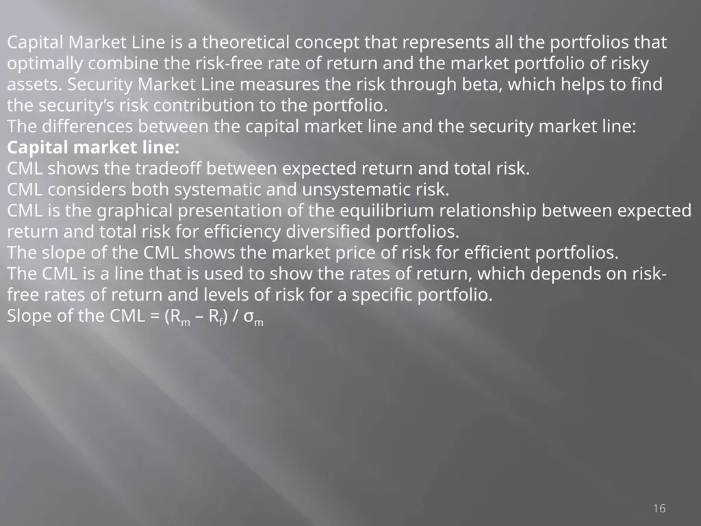
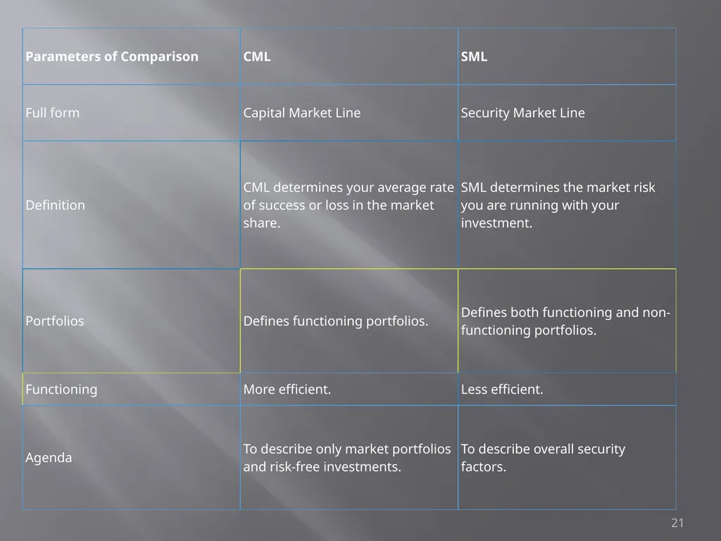
slide16. Capital Market Line is a theoretical concept that represents all the portfolios that optimally combine the risk-free rate of return and the market portfolio of risky assets. Security Market Line measures the risk through beta, which helps to find the security’s risk contribution to the portfolio.
The differences between the capital market line and the security market line:
Capital market line:
CML shows the tradeoff between expected return and total risk.
CML considers both systematic and unsystematic risk.
CML is the graphical presentation of the equilibrium relationship between expected return and total risk for efficiency diversified portfolios.
The slope of the CML shows the market price of risk for efficient portfolios.
The CML is a line that is used to show the rates of return, which depends on risk-free rates of return and levels of risk for a specific portfolio.
Slope of the CML = (Rm – Rf) / σm 16<br>
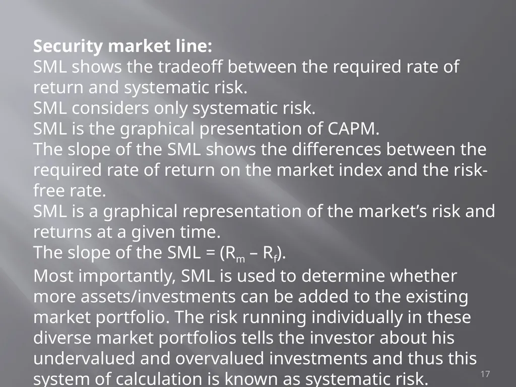
slide17. Security market line:
SML shows the tradeoff between the required rate of return and systematic risk.
SML considers only systematic risk.
SML is the graphical presentation of CAPM.
The slope of the SML shows the differences between the required rate of return on the market index and the risk-free rate.
SML is a graphical representation of the market’s risk and returns at a given time.
The slope of the SML = (Rm – Rf).
Most importantly, SML is used to determine whether more assets/investments can be added to the existing market portfolio. The risk running individually in these diverse market portfolios tells the investor about his undervalued and overvalued investments and thus this system of calculation is known as systematic risk. 17<br>
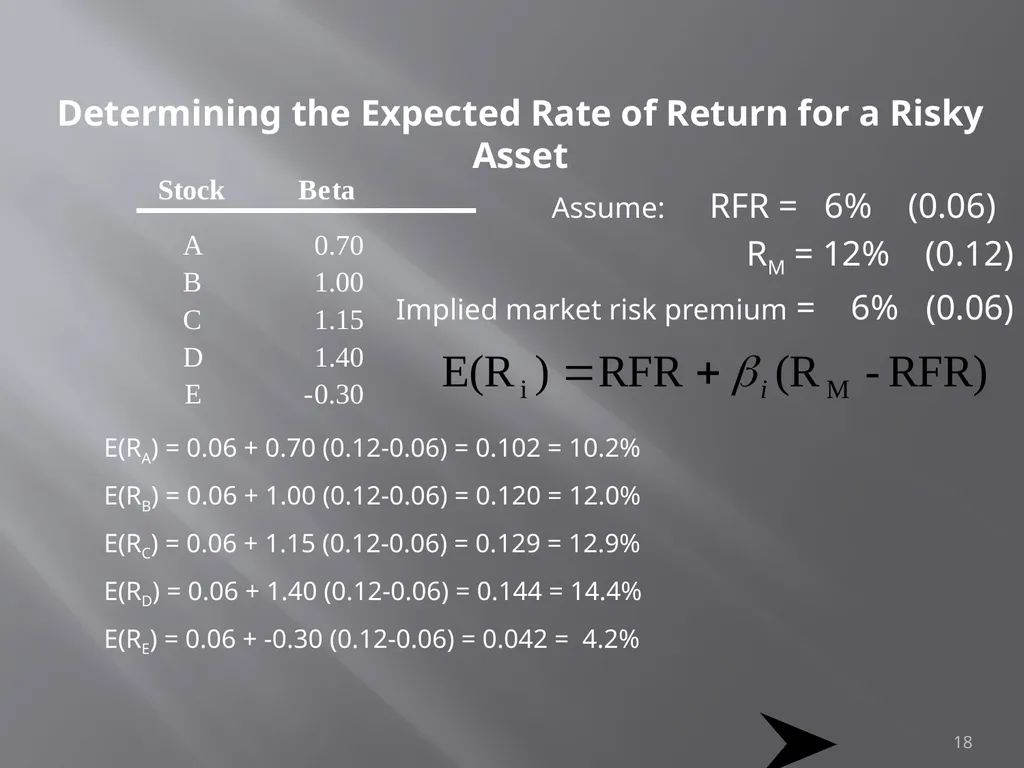
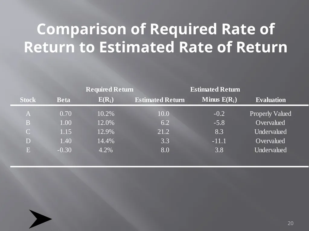
slide18. Determining the Expected Rate of Return for a Risky Asset Assume: RFR = 6% (0.06)
RM = 12% (0.12)
Implied market risk premium = 6% (0.06) 18 E(RA) = 0.06 + 0.70 (0.12-0.06) = 0.102 = 10.2%
E(RB) = 0.06 + 1.00 (0.12-0.06) = 0.120 = 12.0%
E(RC) = 0.06 + 1.15 (0.12-0.06) = 0.129 = 12.9%
E(RD) = 0.06 + 1.40 (0.12-0.06) = 0.144 = 14.4%
E(RE) = 0.06 + -0.30 (0.12-0.06) = 0.042 = 4.2%<br>
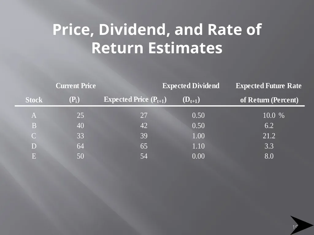
slide19. Price, Dividend, and Rate of Return Estimates 19<br>
slide20. 20 Comparison of Required Rate of Return to Estimated Rate of Return<br>
slide21. 21<br>
slide22. 22 The APT is a more flexible and complex alternative to the Capital Asset Pricing Model (CAPM). The theory provides investors and analysts with the opportunity to customize their research. However, it is more difficult to apply, as it takes a considerable amount of time to determine all the various factors that may influence the price of an asset. Assumptions in the Arbitrage Pricing Theory
The Arbitrage Pricing Theory operates with a pricing model that factors in many sources of risk and uncertainty. Unlike the Capital Asset Pricing Model (CAPM), which only takes into account the single factor of the risk level of the overall market, the APT model looks at several macroeconomic factors that, according to the theory, determine the risk and return of the specific asset.
These factors provide risk premiums for investors to consider because the factors carry systematic risk that cannot be eliminated by diversifying.
The APT suggests that investors will diversify their portfolios, but that they will also choose their own individual profile of risk and returns based on the premiums and sensitivity of the macroeconomic risk factors. Risk-taking investors will exploit the differences in expected and real returns on the asset by using arbitrage.<br>
slide23. 23 Arbitrage in the APT
The APT suggests that the returns on assets follow a linear pattern. An investor can leverage deviations in returns from the linear pattern using the arbitrage strategy. Arbitrage is the practice of the simultaneous purchase and sale of an asset on different exchanges, taking advantage of slight pricing discrepancies to lock in a risk-free profit for the trade. Mathematical Model of the APT
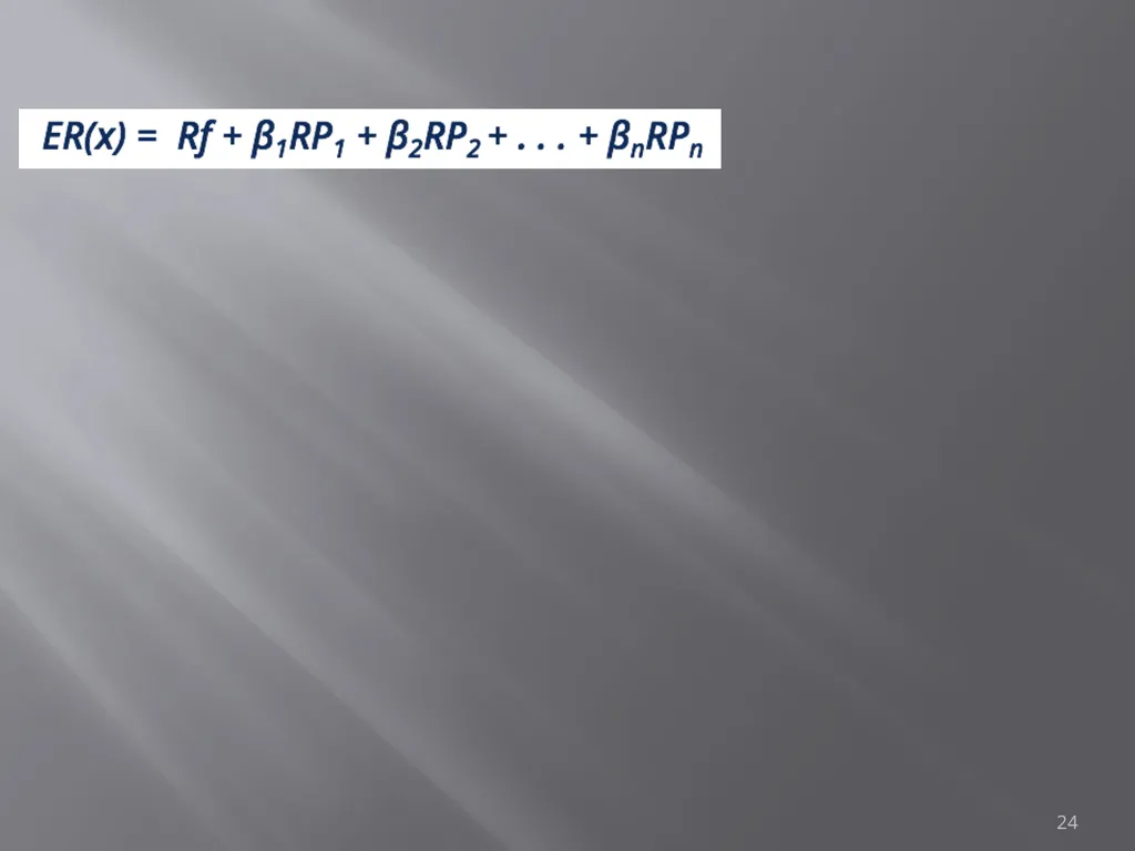
The Arbitrage Pricing Theory can be expressed as a mathematical model:
Where:
ER(x) – Expected return on asset
Rf – Riskless rate of return
βn (Beta) – The asset’s price sensitivity to factor
RPn – The risk premium associated with factor
Historical returns on securities are analyzed with linear regression analysis against the macroeconomic factor to estimate beta coefficients for the arbitrage pricing theory formula<br>
slide24. 24<br>
slide25. If thus the market index is used as a surrogate for other individual securities in the portfolio, the relation of any individual security with the Market index can be represented in a Regression line or characteristic line. This is drawn below, with the excess return on the security on the y-axis and excess return on the Market Portfolio on the x-axis.
The equation of the characteristic line is Ri – Rf = a + βim (Rm – Rf) + ei Ri is the holding period return on security i
Rf is the riskless rate of interest
Alpha is the vertical intercept on y-axis representing the return on the security when only unsystematic risk is considered and systematic risk is measured by Beta. ci is the residual component, not captured by the above variables. 25<br>
slide26. Markowitz Model had serious practical limitations due to the rigours involved in compiling the expected returns, standard deviation, variance, covariance of each security to every other security in the portfolio. Sharpe Model has simplified this process by relating the return in a security to a single Market index. Firstly, this will theoretically reflect all well traded securities in the market. Secondly, it will reduce and simplify the work involved in compiling elaborate matrices of variances as between individual securities. 26<br>
slide27. Rj = αj + βj I+ ej
Where αj is some constant, say risk free return
βj is the Beta which is a risk measure of the market called systematic risk
ADVERTISEMENTS:
I is the value or return on the stock index.
ej is the residual factor which cannot be specified. This optimal portfolio of Sharpe is called the Single Index Model. The optimal portfolio is directly related to the Beta. If Ri is expected return on stock i and Rf is Risk free Rate, then the excess return = Ri – Rf This has to be adjusted to Bi, namely,
Ri – Rf/βi which is the equation for ranking Stocks in the order of their return adjusted for risk.
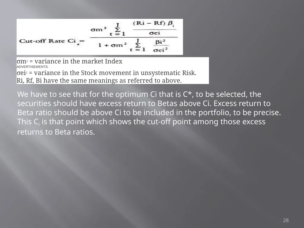
The method involves selecting a cut-off rate for inclusion of securities in a portfolio. For this purpose, excess return to Beta ratio given above has to be calculated for each stock and rank them from highest to lowest. Then only those securities which have Ri – Rf/βi, greater than cut-off point, fixed in advance can be selected.
The basis for finding the cut-off Rate Ci is as follows:
Basis for Cut-off Rate:
For a portfolio of i stocks, Ci is given by cut-off rate- 27<br>
slide28. σm2 = variance in the market Index
ADVERTISEMENTS:
σei2 = variance in the Stock movement in unsystematic Risk.
Ri, Rf, Bi have the same meanings as referred to above. We have to see that for the optimum Ci that is C*, to be selected, the securities should have excess return to Betas above Ci. Excess return to Beta ratio should be above Ci to be included in the portfolio, to be precise. This Ci is that point which shows the cut-off point among those excess returns to Beta ratios. 28<br>
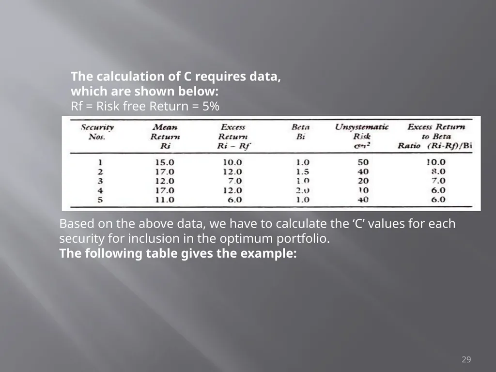
slide29. The calculation of C requires data, which are shown below:
Rf = Risk free Return = 5% Based on the above data, we have to calculate the ‘C’ values for each security for inclusion in the optimum portfolio.
The following table gives the example: 29<br>
slide30. 30<br>
slide31. All securities with excess return to Beta ratio above the cut-off rate C*, say 3.0 in the above table will be chosen in the portfolio. The calculation of cut-off point is also explained. In arriving at the optimal portfolio, the emphasis of Sharpe Model is on Beta and on the Market Index. Sharpe’s optimal portfolio would thus consist of those securities only which have excess return to Beta ratio above a cut-off point.
By this method, selection of the portfolio has become easier due to the ranking of the securities in the order of their excess return and applying the yardstick of a required cut-off point for selection of securities. That cut-off point is related to the excess return to Beta ratio on the one hand and variance of the market index σm2 and variance of the stock’s movement which is related to the unsystematic risk, namely, σei2.
It is thus seen that Sharpe’s Portfolio takes into account both the systematic market related risk and unsystematic risk and residual risk. 31<br>
slide32. The percentage to be invested in each security is- The second expression in the bracket will determine the proportion of funds to be invested in each security. The first expression simply scales the weight on each security, so that the total is summing upto 1. 32<br>
slide33. Portfolio Risk:
When two or more securities or assets are combined in a portfolio, their covariance or interactive risk is to be considered. Thus, if the returns on two assets move together, their covariance is positive and the risk is more on such portfolios. If on the other hand, the returns move independently or in opposite directions, the covariance is negative and the risk in total will be lower.
Mathematically, the covariance is defined as- 33<br>
slide34. o choose the best portfolio from a number of possible portfolios, each with different return and risk, two separate decisions are to be made, det
Determination of a set of efficient portfolios.
Selection of the best portfolio out of the efficient set. 34<br>
slide35. Efficient frontier and Capital Market Line (CML)
An efficient portfolio is one that produces the highest expected return for any given level of risk. Markowitz showed how to find the frontier of risk and returns for stocks. Only portfolios on the frontier are efficient. Sharpe added the riskless asset return and noted that returns on a line connecting rrf and the tangency point on the efficient frontier was also “feasible” in the sense that portfolios consisting of some of the riskless asset and some of the market portfolio could be developed. The introduction of a risk-free asset in the portfolio changes the Markowitz efficient frontier into a straight line. He called that straight efficient frontier line the Capital Market Line (CML), and he used indifference curves to show how investors with different degrees of risk aversion would choose portfolios with different mixes of stocks and the riskless asset. Investors who are not at all averse to risk could borrow and buy stocks on margin, and thus move out the CML beyond the tangency point. Since the line is straight, the math implies that any two assets falling on this line will be perfectly positively correlated with each other. 35<br>
slide36. 36<br>
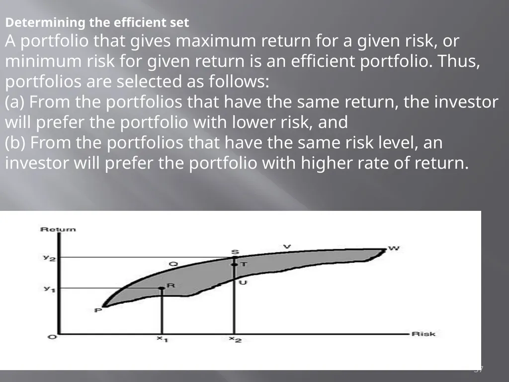
slide37. Determining the efficient set
A portfolio that gives maximum return for a given risk, or minimum risk for given return is an efficient portfolio. Thus, portfolios are selected as follows:
(a) From the portfolios that have the same return, the investor will prefer the portfolio with lower risk, and
(b) From the portfolios that have the same risk level, an investor will prefer the portfolio with higher rate of return. 37<br>
slide38. As the investor is rational, they would like to have higher return. And as they are risk averse, they want to have lower risk. In Figure 1, the shaded area PVWP includes all the possible securities an investor can invest in. The efficient portfolios are the ones that lie on the boundary of PQVW. For example, at risk level x2, there are three portfolios S, T, U. But portfolio S is called the efficient portfolio as it has the highest return, y2, compared to T and U[needs dot]. All the portfolios that lie on the boundary of PQVW are efficient portfolios for a given risk level. 38<br>
slide39. The boundary PQVW is called the Efficient Frontier. All portfolios that lie below the Efficient Frontier are not good enough because the return would be lower for the given risk. Portfolios that lie to the right of the Efficient Frontier would not be good enough, as there is higher risk for a given rate of return. All portfolios lying on the boundary of PQVW are called Efficient Portfolios. The Efficient Frontier is the same for all investors, as all investors want maximum return with the lowest possible risk and they are risk averse. 39<br>
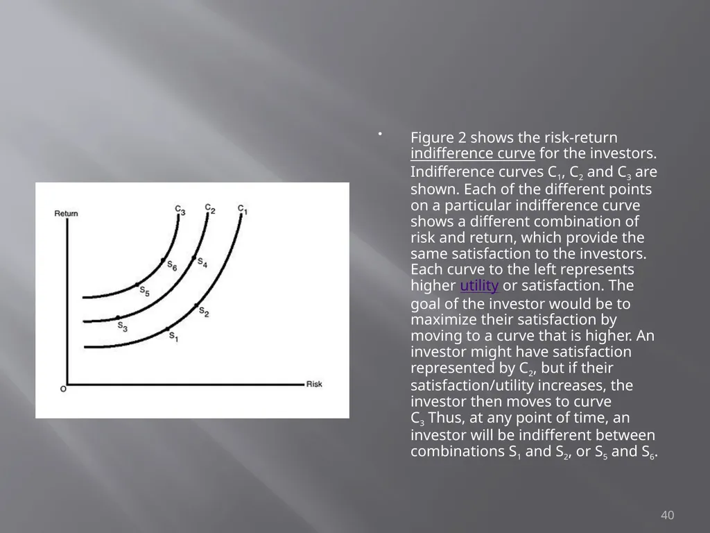
slide40. Figure 2 shows the risk-return indifference curve for the investors. Indifference curves C1, C2 and C3 are shown. Each of the different points on a particular indifference curve shows a different combination of risk and return, which provide the same satisfaction to the investors. Each curve to the left represents higher utility or satisfaction. The goal of the investor would be to maximize their satisfaction by moving to a curve that is higher. An investor might have satisfaction represented by C2, but if their satisfaction/utility increases, the investor then moves to curve C3 Thus, at any point of time, an investor will be indifferent between combinations S1 and S2, or S5 and S6. 40<br>
slide41. The investor's optimal portfolio is found at the point of tangency of the efficient frontier with the indifference curve. This point marks the highest level of satisfaction the investor can obtain. 41<br>
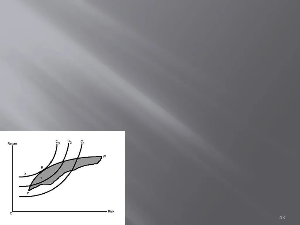
slide42. The investor's optimal portfolio is found at the point of tangency of the efficient frontier with the indifference curve. This point marks the highest level of satisfaction the investor can obtain. This is shown in Figure 3. R is the point where the efficient frontier is tangent to indifference curve C3, and is also an efficient portfolio. With this portfolio, the investor will get highest satisfaction as well as best risk-return combination (a portfolio that provides the highest possible return for a given amount of risk). Any other portfolio, say X, isn't the optimal portfolio even though it lies on the same indifference curve as it is outside the feasible portfolio available in the market. Portfolio Y is also not optimal as it does not lie on the best feasible indifference curve, even though it is a feasible market portfolio. Another investor having other sets of indifference curves might have some different portfolio 42<br>
slide43. 43<br>
slide44. 44<br>
slide45. 45<br>
slide46. 46<br>
slide47. This Exhibit demonstrates that it is possible to eliminate risk—that is, to achieve zero variance—with a portfolio of two perfectly positively correlated stocks. To do this, it is necessary to be long in one investment and short in the other in proportions that place the portfolio at point C. 47<br>
slide48. Forming a Riskless Portfolio from Two Perfectly Negatively Correlated Securities with perfect positive correlation, the standard deviation of a portfolio with positive weights on both stocks equals the portfolio-weighted average of the two standard deviations. Now, consider the case where risky investments have less than perfect correlation (p < 1).The states that the lower the correlation, the lower the portfolio variance. Therefore, the standard deviation of a portfolio with positive weights on both stocks is less than the portfolio-weighted average of the two standard deviations, which gives the curvature to the left shown in Exhibit 4.5. The degree to which this curvature occurs depends on the correlation between the returns. Consistent with Result 4.2, the smaller the correlation, p, the more distended the curvature. The ultimate in curvature is the pair of lines generated with perfect negative correlation, p = -1, which is the smallest correlation possible. 48<br>
slide49. An optimal stock portfolio refers to a stock portfolio that incorporates the stocks configured in such a manner that they yield the optimal return statistically possible at a given level of risk accepted by an investor. The modern portfolio theory stresses on the optimal portfolio concept by assuming that the investors try to minimize risk obsessively while looking for the highest return possible. As per this theory, investors should make rational decisions for achieving maximum returns at their acceptable level of risk.
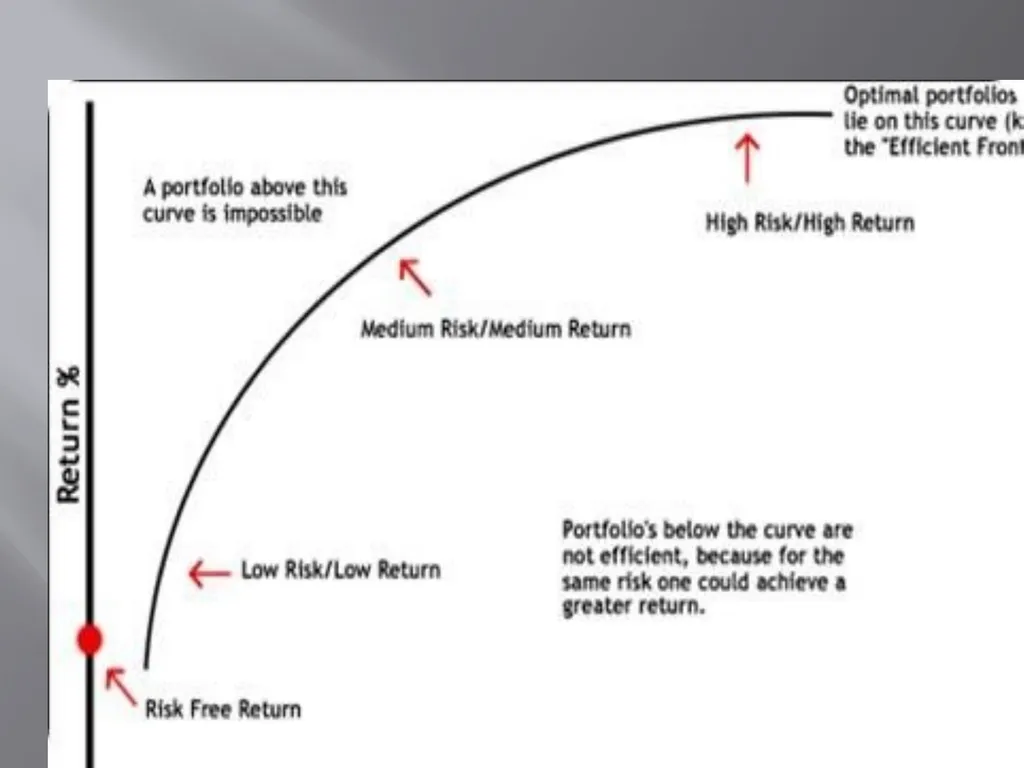
The working of the optimal portfolio can be easily understood by looking at the chart below. The optimal-risk portfolio is generally found in the middle of the curve. If one goes further higher up the curve, it will mean taking more risk proportionately for achieving lower incremental return. Similarly if one goes at lower end of the curve, it will mean low risk/low return portfolios. 49<br>
slide50. 50<br>
slide51. Sources and Types of Risk Sources of Risk:
Interest rate risk
Market risk
Inflation risk
Business risk
Financial risk
Liquidity risk
Exchange rate risk
Country risk
Broad Types:
Systematic/Market Risk
Non-systematic/Non-market/Company-specific Risk 51<br>
slide52. 52<br>
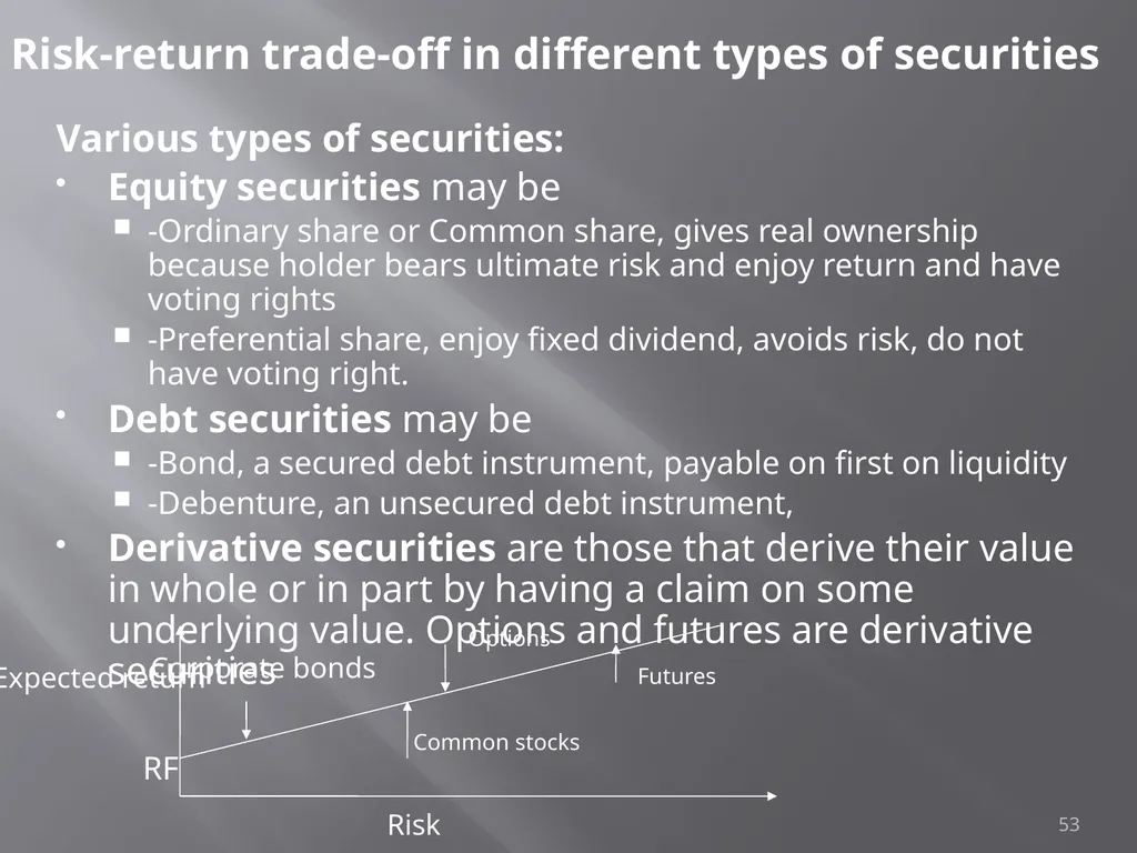
slide53. Risk-return trade-off in different types of securities Various types of securities:
Equity securities may be
-Ordinary share or Common share, gives real ownership because holder bears ultimate risk and enjoy return and have voting rights
-Preferential share, enjoy fixed dividend, avoids risk, do not have voting right.
Debt securities may be
-Bond, a secured debt instrument, payable on first on liquidity
-Debenture, an unsecured debt instrument,
Derivative securities are those that derive their value in whole or in part by having a claim on some underlying value. Options and futures are derivative securities Corporate bonds Common stocks Options Futures RF Expected return Risk 53<br>
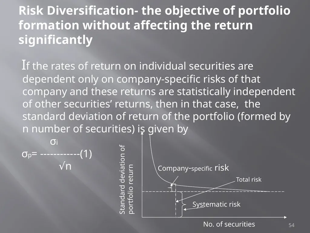
slide54. Risk Diversification- the objective of portfolio formation without affecting the return significantly If the rates of return on individual securities are dependent only on company-specific risks of that company and these returns are statistically independent of other securities’ returns, then in that case, the standard deviation of return of the portfolio (formed by n number of securities) is given by
σi
σp= ------------(1)
√n Standard deviation of portfolio return No. of securities Systematic risk Company-specific risk Total risk 54<br>
slide55. Risk Diversification Risk diversification is the key to the management of portfolio risk, because it allows investors to significantly lower the portfolio risk without adversely affecting return.
Diversification types:
Random or naive diversification
Efficient diversification 55<br>
slide56. Random or naive diversification: It refers to the act of randomly diversifying without regard to relevant investment characteristics such as expected return and industry classification. An investor simply selects relatively large number of securities randomly.
Unfortunately, in such case, the benefits of random diversification do not continue as we add more securities, the reduction becomes smaller and smaller. 56<br>
slide57. Efficient diversification Efficient diversification takes place in an efficient portfolio that has the smallest portfolio risk for a given level of expected return or the largest expected return for a given level of risk. Investors can specify a portfolio risk level they are willing to assume and maximize the expected return on the portfolio for this level of risk.
Rational investors look for efficient portfolios, because these portfolios are optimized on the two dimensions of most importance to investors- return and risk. 57<br>
slide58. Modern Portfolio Theory In 1952, Markowitz, the father of modern portfolio theory, developed the basic principle of portfolio diversification in a formal way, in quantified form, that shows why and how portfolio diversification works to reduce the risk of a portfolio to an investor. Modern Portfolio theory hypothesizes how investors should behave.
According to Markowitz, the portfolio risk is not simply a weighted average of the risks brought by individual securities in the portfolio but it also includes the risks that occurs due to correlations among the securities in the portfolio. As the no. of securities in the portfolio increases, contribution of individual security’s risk decreases due to offsetting effect of strong performing and poor performing securities in the portfolio and the importance of covariance relationships among securities increases. Thus the portfolio risk is given by
σ2p=∑wi2σi2 + ∑ ∑wiwjρijσiσj
=∑ ∑wiwjρijσiσj (the 1st term is neglected for large n) 58<br>
slide59. Efficient Frontiers Risk σ E ( R ) A Global minimum portfolio C B Portfolio on AB section are better than those on AC in risk-return perspective and so portfolios on AB are called efficient portfolios that offers best risk-return combinations to investors Graph for the risk-return trade-off according to Markowitz portfolio theory is
drawn below. 59<br>
slide60. Computing Problem with Original Markowitz Theory, and Later Simplification As n increases, n(n-1) covariances (inputs) are required to calculate under Markowitz model. Due to this complexity of computation, it was mainly used for academic purposes before simplification.
It was observed that mirror images of covariances were present in Markowitz’s model. So after excluding the mirror images in the simplified form, n(n-1)/2 unique covariances are required for using this model and since then it is being used by investors. 60<br>
slide61. How to Calculate Portfolio Standard Deviation?
Portfolio Standard Deviation calculation is a multi-step process and involves the below-mentioned process.
Portfolio Standard Deviation Formula
Assuming a Portfolio comprising of two assets only, the Standard Deviation of a Two Asset Portfolio can be computed using Portfolio Standard Deviation Formula:
Find the Standard Deviation of each asset in the portfolio
Find the weight of each asset in the overall portfolio
Find the correlation between the assets in the portfolio (in the above case between the two assets in the portfolio). Correlation can vary in the range of -1 to 1.
Apply the values in the above-mentioned to derive the Standard Deviation formula of a Two Asset Portfolio. 61<br>
slide62. What is a Portfolio ? A portfolio refers to a collection of investment tools such as stocks, shares, mutual funds, bonds, cash and so on depending on the investor’s income, budget and convenient time frame. 62<br>
slide63. What is Portfolio Management ? The art of selecting the right investment policy for the individuals in terms of minimum risk and maximum return is called as portfolio management.
Portfolio management refers to managing an individual’s investments in the form of bonds, shares, cash, mutual funds etc so that he earns the maximum profits within the stipulated time frame.
Portfolio management refers to managing money of an individual under the expert guidance of portfolio managers.
In a layman’s language, the art of managing an individual’s investment is called as portfolio management. 63<br>
slide64. Need for Portfolio Management Portfolio management presents the best investment plan to the individuals as per their income, budget, age and ability to undertake risks.
Portfolio management minimizes the risks involved in investing and also increases the chance of making profits.
Portfolio managers understand the client’s financial needs and suggest the best and unique investment policy for them with minimum risks involved.
Portfolio management enables the portfolio managers to provide customized investment solutions to clients as per their needs and requirements. 64<br>
slide65. Types of Portfolio Management Portfolio Management is further of the following types:
Active Portfolio Management: As the name suggests, in an active portfolio management service, the portfolio managers are actively involved in buying and selling of securities to ensure maximum profits to individuals.
Passive Portfolio Management: In a passive portfolio management, the portfolio manager deals with a fixed portfolio designed to match the current market scenario.
Discretionary Portfolio management services: In Discretionary portfolio management services, an individual authorizes a portfolio manager to take care of his financial needs on his behalf. The individual issues money to the portfolio manager who in turn takes care of all his investment needs, paper work, documentation, filing and so on. In discretionary portfolio management, the portfolio manager has full rights to take decisions on his client’s behalf.
Non-Discretionary Portfolio management services: In non discretionary portfolio management services, the portfolio manager can merely advise the client what is good and bad for him but the client reserves full right to take his own decisions. 65<br>
slide66. traditional portfolio analysis has been of a very subjective nature but it has provided success to some persons who have made their investments by making analysis of individual securities through evaluation of return and risk conditions in each security. The modern portfolio theory believes in the maximization of return through a combination of securities. The modern portfolio theory discusses the relationship between different securities and then draws inter-relationships of risks between them. 66<br>
slide67. Traditional theory was based on the fact that risk could be measured on each individual security through the process of finding out the standard deviation and that security should be chosen where the deviation was the lowest. Greater variability and higher deviations showed more risk than those securities which had lower variation. The modern theory is of the view that by diversification risk can be reduced. Diversification can be made by the investor either by having a large number of shares of companies in different regions,. Diversification is important but the modern theory states that there cannot be only diversification to achieve the maximum return. The theory of diversification was based on the research work by Harry Markowitz. 67<br>
slide68. Traditional theory believes that the market is inefficient and the fundamental analyst can take advantage of the situation. By analysing internal financial statements of the company, he can make superior profits through higher returns. The technical analyst believed in the market behaviour and past trends to forecast the future of the securities. These analyses were mainly under the risk and return criteria of single security analysis. Modern portfolio theory, as brought out by Markowitz and Sharpe, is the combination of the securities to get the most efficient portfolio. Combination of securities can be made in many ways. Markowitz developed the theory of diversification through scientific reasoning and method. 68<br>
slide69. Harry Markowitz’s Modern Portfolio Theory in 1952, an economist named Harry Markowitz wrote his dissertation on “Portfolio Selection”, a paper that contained theories which transformed the landscape of portfolio management—a paper which would earn him the Nobel Prize in Economics nearly four decades later.
As the philosophical antithesis of traditional stock selection, his Modern Portfolio Theory (MPT) continues to be a popular investment strategy, and this portfolio management tool—if used correctly—can result in a diverse, profitable investment portfolio.
Instead of focusing on the risk of each individual asset, Markowitz demonstrated that a diversified portfolio is less volatile than the total sum of its individual parts. While each asset itself might be quite volatile, the volatility of the entire portfolio can actually be quite low.
More than 60 years after its introduction, the fundamentals of MPT ring true. Let’s delve into this popular portfolio management strategy, and discover what makes the principles of this revolutionary theory so effective. 69<br>
slide70. Prior to the development of MPT, investing processes were centered on individual stocks; investors would look through available assets and find “sure bets”—assets that would produce decent returns without subjecting the investor to too much risk. Expected net present value (NPV) was used to distinguish these “sure bet” stocks, while securities were valued by discounting their future cash flows. Stocks that were capable of generating more money at a quicker rate were given great value. Markowitz disagreed with this thinking. The “present value” theory had shortcomings; selecting the “best” portfolio under this logic meant selecting a single stock with the highest expected NPV. That approach was risky by nature, and while economic experts believed a good portfolio was a diversified one, there was no methodology available for investors to achieve this diversity. 70<br>
slide71. 71<br>
slide72. What is MPT? Markowitz created a formula that allows an investor to mathematically trade off risk tolerance and reward expectations, resulting in the ideal portfolio.
This theory was based on two main concepts:
1. Every investor’s goal is to maximize return for any level of risk 2. Risk can be reduced by diversifying a portfolio through individual, unrelated securities
MPT works under the assumption that investors are risk-averse, preferring a portfolio with less risk for a given level of return. Under this assumption, investors will only take on high-risk investments if they can expect a larger reward. 72<br>
slide73. What is Modern Portfolio Theory?
An investment model like modern portfolio theory or MPT allows investors to choose from a variety of investment options comprising of a single portfolio for earning maximum benefits and that too at a market risk which is way lower than the various underlying investments or assets.
Explanation
Modern Portfolio Theory (MPT) is an investing model in which investors invest with the motive of taking the minimum level of risk and earning the maximum amount of return for that level of acquired risk. The modern portfolio theory is a helpful tool for the investors as it helps them in choosing the different types of investments for the purpose of the diversification of the investment and then making one portfolio by considering all the investments.
According to the modern portfolio theory, all the investments that are selected are combined together in a way that reduces the risk in the market through the means of diversification and, at the same time, also generates a good return in the long term to the investors.
Example of the Modern Portfolio Theory (MPT)
There is an individual who wants to invest in a portfolio. He got an option of two portfolios, which are as follows:
The first portfolio consists of a mix of the bonds and different stocks that gave the return of 10 % annually on an average, but at the same time differed by the range of as much as 15 % annually (returns, in this case, usually differed between -5 % and + 25 %).
On the other hand, the second portfolio consists of a mix of the bonds and different stocks that gave the return of 10 % annually on an average, but at the same time differed by a range of only 3 % annually (returns, in this case, usually differed between 7 % and 13 %)
According to modern portfolio theory, which investment portfolio the person should consider?
Analysis
In both scenarios, the average expected return on the investment is 10 %. However, in the first portfolio, one could get the return of as much as 25 %, which sounds attractive, but at the same time, there prevails a huge risk where one might lose 5 % as well because the range usually differs between -5 % and + 25 %.
On the other side, in the case of the second portfolio, a less return range of between 7 % and 13 % may be less attractive to the investor, but in that case, it is expected that one will not lose his money, which makes the investment less risky than the first portfolio.
According to the Modern portfolio, theory investor invests with the motive of taking the minimum level of risk and earning the maximum amount of return with that minimum risk taken, so in the present case, one should choose the second portfolio as he is getting the same average expected return with the less level of risk.
Assumptions of Modern Portfolio Theory
Modern Portfolio theory has a certain assumption that is to be considered while making any decisions in order to arrive at the conclusion that risk, return, and diversification relationships hold true. The different assumptions of the modern portfolio theory are as follows:
Returns from the assets are distributed normally.
The investor making the investment is rational and will avoid all the unnecessary risk associated.
Investors will give their best in order to maximize returns for all the unique situations provided.
All investors are having access to the same information.
The cost pertaining to taxes and trading is not considered while making decisions.
All the investors are having the same views on the rate of return expected.
The single investors along are not sizeable and capable enough to influence the prices prevailing in the market.
Unlimited capital at the risk-free rate of return can be borrowed.
Advantages of the Modern Portfolio Theory (MPT)
There are several different advantages of the Modern portfolio theory providing the opportunity for the investors investing their money in the market. Some of the advantages are of the Modern portfolio theory as follows:
It helps in evaluating and managing risks and returns associated with the investments. With the help of analysis, the assets which are underperforming assets and the assets having an excessive risk with respect to returns can be scrutinized and then replaced with the new one.
The theory is an important tool for avoiding financial ruin because by following these theories, traders don’t rely on only one investment for their financial stability; rather, they diversify their portfolio in order to get the maximum return with minimum risk. 73<br>
slide74. Disadvantages of the Modern Portfolio Theory (MPT)
Along with the different advantages, there exist the limitations and drawbacks also of the Modern portfolio theory, which includes the following:
In the case of the modern portfolio theory, the past performance of the company under consideration is taken. The performance of the past never provides a guarantee for the result that could arise in the future. Considering only the past performances sometimes leads to overpassing the newer circumstances, which might not be there when historical data were considered but could play an important role in making the decision.
This theory assumes that there is a normal distribution of the return on an asset within a class of assets, which is proved to be wrong for individual equities as the correlations of asset class may change over the period of time.
In this theory, there is an assumption that securities of any of the sizes can be bought and sold, which doesn’t hold true as some of the securities have minimum order sizes, which cannot be dealt with in the fraction.
Modern Portfolio Theory even though is accepted widely all over the world and also applied by different investment institution, but at the same time it has also been criticized by different persons particularly by representatives of the behavioral economics who challenges the assumptions of the Modern portfolio theory on the parameters of investor rationality and the expectations for the return.
Conclusion
The main idea or the purpose of the Modern portfolio theory says that the risk is undertaken and return expected linked directly, which means that in order to achieve the greater rate of expected returns, an investor must have to take a higher level of risk. Also, the theory says that the overall risk of the portfolio having securities can be reduced through the means of diversification. In case two different portfolios are given to the investor having the same level of expected return, then the rational decision would be to choose the portfolio having lower total risk.
Modern Portfolio Theory, even though it is accepted widely all over the world and also applied by different investment institutions, but at the same time, it has also been criticized by different persons. However, regardless of the different criticism, Modern portfolio theory is a working strategy having a diversified investment that is implemented by different risk managers, investment institutions, and related persons. 74<br>
slide2. Systematic Risk vs. Unsystematic Risk Systematic Risk – These are market risks—that is, general perils of investing—that cannot be diversified away.
Interest rates, recessions, and wars are examples of systematic risks.
Unsystematic Risk – Also known as "specific risk," this risk relates to individual stocks. In more technical terms, it represents the
component of a stock's return that is not correlated with general market moves. Modern portfolio theory shows that specific risk can be removed or at least mitigated through diversification of a portfolio. The trouble is that diversification still does not solve the problem of systematic risk; even a portfolio holding all the shares in the stock market can't eliminate that risk. Therefore, when calculating a deserved return, systematic risk is what most plagues investors. The capital asset pricing model was developed by the financial economist (and later, Nobel laureate in economics) William Sharpe, set out in his 1970 book Portfolio Theory and Capital Markets. His model starts with the idea that individual investment contains two types of risk: 2<br>
slide3. 3<br>
slide4. The capital asset pricing model (CAPM) is the equation that describes the relationship between the expected return of a given security and systematic risk as measured by its beta coefficient. Besides risk the model considers the effect of risk-free interest rates and expected market return.
Assumptions
Basic assumptions of the CAPM model are as follows.
Markets are ideal—no transaction fees, taxes, inflation, or short selling restrictions.
All investors are averse to risk.
Markets are highly efficient. All investors have equal access to all available information.
All investors can borrow and lend unlimited amounts under a risk-free rate.
Beta coefficient is the only measure of risk.
All assets are absolutely liquid and infinitely divided.
The amount of available assets is fixed during a given period of time.
Markets are in equilibrium. All investors are price takers, not price makers.
Return of all available assets is subject to normal distribution function. 4<br>
slide5. 5<br>
slide6. The Capital Asset Pricing Model (CAPM) measures the risk of a security in relation to the portfolio. It considers the required rate of return of a security in the light of its contribution to total portfolio risk. The CAPM holds that only undiversifiable risk is relevant to the determination of expected return on any asset.
Even though the CAPM is competent to examine the risk and return of any capital asset such as individual security, an investment project or a portfolio asset 6<br>
slide7. Assumptions of Capital Asset Pricing Model
The CAPM is based on the following assumptions.
1. Risk-averse investors
The investors are basically risk averse and diversification is necessary to reduce their risks.
2. Maximising the utility of terminal wealth
An investor aims at maximizing the utility of his wealth rather than the wealth or return. The term ‘Utility’ describes the differences in individual preferences. Each increment of wealth is enjoyed less than the last as each increment is less important in satisfying the basic needs of the individual. Thus, the diminishing marginal utility is most applicable to wealth.
There are also other forms of utility functions. Some investors showing a preference for larger risks are those who have increasing marginal utility for wealth. In such cases, each increase in wealth prompts the individual to acquire more wealth. For a risk-neutral investor, each increment in wealth is equally attractive. In other words, each increment would have the same utility for him. 7<br>
slide8. 3. Choice on the basis of risk and return:
Investors make investment decisions on the basis of risk and return. Risk and return are measured by the variance and the mean of the portfolio returns. CAPM assumes that the rational investors put away their diversifiable risk, namely, unsystematic risk. But only the systematic risk remains which varies with the Beta of the security.
Some investors use the beta only to measure the risk while other investors use both beta and variance of returns as the sources of reward. As individuals have varying perceptions towards risk and reward, CAPM gives a series of efficient frontlines. 4. Similar expectations of risk and return
All investors have similar expectations of risk and return. In other words, all investors’ estimates of risk and return are the same. When the expectations of the investors differ, the estimates of mean and variance lead to different forecasts.
As a result, there will be innumerable efficient frontiers and the efficient portfolio of each will be different from that of the others. Varying preferences also imply that the price of an asset will be different for different investors. 5. Identical time horizon
The CAPM is based on the assumption that all investors have identical time horizon. The core of this assumption is that investors buy all the assets in their portfolios at one point of time and sell them at some undefined but common point in future. This assumption further implies that investors form portfolios to achieve wealth at a single common terminal rate. 8<br>
slide9. 6. Free access to all available information
One of the important assumptions of the CAPM is that investors have free access to all the available information at no cost. Supposing some investors alone are able to have access to special information which is not readily available to all, then the markets would not be regarded efficient. In other words, if the available information has not reached all, it will be difficult to draw a common efficient frontier line. 7. There is risk-free asset and there is no restriction on borrowing and lending at the risk free rate
This is a very important assumption of the CAPM. The risk free asset is essential to simplify the complex pairwise covariance of Markowitz’s theory. The risk free asset makes the curved efficient frontier of MPT to the linear efficient frontier of the CAPM simple.
As a result, the investors will not concentrate on the characteristics of individual assets. By adding a portion of risk-free assets to the portfolio and borrowing the additional funds needed at a risk free rate, the risk is either decreased or increased. 8. There are no taxes and transaction costs
According to Roll, there must be either a risk free asset or a portfolio of short sold securities. Then only the capital Market Line (CML) will be straight. When there are no risk free assets, the investor could not create a proxy risk free asset. As a result, the capital market line would not be linear and the direct linear relationship between risk and return would not exist. 9. Total availability of assets is fixed and assets are marketable and divisible
This assumption holds the view that the total asset quantity is fixed and all assets are marketable. 9<br>
slide10. Formula
The CAPM model allows you to assess the expected return of a given security using the following formula:
E(Ri) = RF + βi × (E(RM) - RF)
where E(Ri) is an expected return of a security, RF is a risk-free rate, βi is the beta coefficient of a security, and E(RM) is an expected Market risk premium (RPM) can be calculated as follows.
RPM) = E(RM) - RF
The risk premium of a given security (RPi) can be assessed as follows:RPi) = βi × (E(RM) - RF)
Example
Let’s assume an investor is thinking of buying one of three stocks: Stock A with a beta of 0.85, Stock B with a beta of 1.25, and Stock C with a beta of 1.65. If the risk-free rate is 4.50% and the expected market return is 12.35%, the expected return of each security can be assessed under CAPM. E(RA) = 4.50 + 0.85 × (12.35 - 4.50) = 11.17%
E(RB) = 4.50 + 0.85 × (12.35 - 4.50) = 14.31%
E(RC) = 4.50 + 0.85 × (12.35 - 4.50) = 17.45%
Thus, a relationship exists between risk and the expected return of a security. So, the higher the beta, the higher the expected return and vice versa. 10<br>
slide11. CAPM's starting point is the risk-free rate–typically a 10-year government bond yield. A premium is added, one that equity investors demand as compensation for the extra risk they accrue. This equity market premium consists of the expected return from the market as a whole less the risk-free rate of return. The equity risk premium is multiplied by a coefficient that Sharpe called "beta." Beta's Role in CAPM
According to CAPM, beta is the only relevant measure of a stock's risk. It measures a stock's relative volatility–that is, it shows how much the price of a particular stock jumps up and down compared with how much the entire stock market jumps up and down. If a share price moves exactly in line with the market, then the stock's beta is 1. A stock with a beta of 1.5 would rise by 15% if the market rose by 10% and fall by 15% if the market fell by 10%. Beta, compared with the equity risk premium, shows the amount of compensation equity investors need for taking on additional risk. If the stock's beta is 2.0, the risk-free rate is 3%, and the market rate of return is 7%, the market's excess return is 4% (7% - 3%). Accordingly, the stock's excess return is 8% (2 x 4%, multiplying market return by the beta), and the stock's total required return is 11% (8% + 3%, the stock's excess return plus the risk-free rate). What the beta calculation shows is that a riskier investment should earn a premium over the risk-free rate. The amount over the risk-free rate is calculated by the equity market premium multiplied by its beta. In other words, it is possible, by knowing the individual parts of the CAPM, to gauge whether or not the current price of a stock is consistent with its likely return. 11<br>
slide12. 12<br>
slide13. Portfolio diversification
CAPM deals with the risks and returns on financial securities and defines them precisely, if arbitrarily. The rate of return an investor receives from buying a common stock and holding it for a given period of time is equal to the cash dividends received plus the capital gain (or minus the capital loss) during the holding period divided by the purchase price of the security.
Although investors may expect a particular return when they buy a particular stock, they may be disappointed or pleasantly surprised, because fluctuations in stock prices result in fluctuating returns. Therefore common stocks are considered risky securities. (In contrast, because the returns on some securities, such as Treasury bills, do not differ from their expected returns, they are considered riskless securities.) Financial theory defines risk as the possibility that actual returns will deviate from expected returns, and the degree of potential fluctuation determines the degree of risk.
An underpinning of CAPM is the observation that risky stocks can be combined so that the combination (the portfolio) is less risky than any of its components. Although such diversification is a familiar notion, it may be worthwhile to review the manner in which diversification reduces risk. 13<br>
slide14. The security market line
The culmination of the sequence of conceptual building blocks is CAPM’s risk/expected return relationship. This fundamental result follows from the proposition that only systematic risk, measured by beta (β), matters. Securities are priced such that:
Rs = Rf + risk premium
Rs = Rf + βs (Rm – Rf)
Where: Rs = the stock’s expected return (and the company’s cost of equity capital).
Rf = the risk-free rate.
Rm = the expected return on the stock market as a whole.
β s = the stock’s beta.
This risk/expected return relationship is called the security market line (SML). I have illustrated it graphically in Exhibit III. As I indicated before, the expected return on a security generally equals the risk-free rate plus a risk premium. In CAPM the risk premium is measured as beta times the expected return on the market minus the risk-free rate. The risk premium of a security is a function of the risk premium on the market, Rm – Rf, and varies directly with the level of beta. (No measure of unsystematic risk appears in the risk premium, of course, for in the world of CAPM diversification has eliminated it.) 14 Security Market Line Slope
The slope of the security market line represents the market risk premium, i.e. the excess return over the market return. The market risk premium compensates for the additional systematic risk associated with the security. Therefore, the higher the risk, the higher the market risk premium for the security, and the higher the expected overall return for the security.<br>
slide15. In the freely competitive financial markets described by CAPM, no security can sell for long at prices low enough to yield more than its appropriate return on the SML. The security would then be very attractive compared with other securities of similar risk, and investors would bid its price up until its expected return fell to the appropriate position on the SML. Conversely, investors would sell off any stock selling at a price high enough to put its expected return below its appropriate position. The resulting reduction in price would continue until the stock’s expected return rose to the level justified by its systematic risk. 15<br>
slide16. Capital Market Line is a theoretical concept that represents all the portfolios that optimally combine the risk-free rate of return and the market portfolio of risky assets. Security Market Line measures the risk through beta, which helps to find the security’s risk contribution to the portfolio.
The differences between the capital market line and the security market line:
Capital market line:
CML shows the tradeoff between expected return and total risk.
CML considers both systematic and unsystematic risk.
CML is the graphical presentation of the equilibrium relationship between expected return and total risk for efficiency diversified portfolios.
The slope of the CML shows the market price of risk for efficient portfolios.
The CML is a line that is used to show the rates of return, which depends on risk-free rates of return and levels of risk for a specific portfolio.
Slope of the CML = (Rm – Rf) / σm 16<br>
slide17. Security market line:
SML shows the tradeoff between the required rate of return and systematic risk.
SML considers only systematic risk.
SML is the graphical presentation of CAPM.
The slope of the SML shows the differences between the required rate of return on the market index and the risk-free rate.
SML is a graphical representation of the market’s risk and returns at a given time.
The slope of the SML = (Rm – Rf).
Most importantly, SML is used to determine whether more assets/investments can be added to the existing market portfolio. The risk running individually in these diverse market portfolios tells the investor about his undervalued and overvalued investments and thus this system of calculation is known as systematic risk. 17<br>
slide18. Determining the Expected Rate of Return for a Risky Asset Assume: RFR = 6% (0.06)
RM = 12% (0.12)
Implied market risk premium = 6% (0.06) 18 E(RA) = 0.06 + 0.70 (0.12-0.06) = 0.102 = 10.2%
E(RB) = 0.06 + 1.00 (0.12-0.06) = 0.120 = 12.0%
E(RC) = 0.06 + 1.15 (0.12-0.06) = 0.129 = 12.9%
E(RD) = 0.06 + 1.40 (0.12-0.06) = 0.144 = 14.4%
E(RE) = 0.06 + -0.30 (0.12-0.06) = 0.042 = 4.2%<br>
slide19. Price, Dividend, and Rate of Return Estimates 19<br>
slide20. 20 Comparison of Required Rate of Return to Estimated Rate of Return<br>
slide21. 21<br>
slide22. 22 The APT is a more flexible and complex alternative to the Capital Asset Pricing Model (CAPM). The theory provides investors and analysts with the opportunity to customize their research. However, it is more difficult to apply, as it takes a considerable amount of time to determine all the various factors that may influence the price of an asset. Assumptions in the Arbitrage Pricing Theory
The Arbitrage Pricing Theory operates with a pricing model that factors in many sources of risk and uncertainty. Unlike the Capital Asset Pricing Model (CAPM), which only takes into account the single factor of the risk level of the overall market, the APT model looks at several macroeconomic factors that, according to the theory, determine the risk and return of the specific asset.
These factors provide risk premiums for investors to consider because the factors carry systematic risk that cannot be eliminated by diversifying.
The APT suggests that investors will diversify their portfolios, but that they will also choose their own individual profile of risk and returns based on the premiums and sensitivity of the macroeconomic risk factors. Risk-taking investors will exploit the differences in expected and real returns on the asset by using arbitrage.<br>
slide23. 23 Arbitrage in the APT
The APT suggests that the returns on assets follow a linear pattern. An investor can leverage deviations in returns from the linear pattern using the arbitrage strategy. Arbitrage is the practice of the simultaneous purchase and sale of an asset on different exchanges, taking advantage of slight pricing discrepancies to lock in a risk-free profit for the trade. Mathematical Model of the APT
The Arbitrage Pricing Theory can be expressed as a mathematical model:
Where:
ER(x) – Expected return on asset
Rf – Riskless rate of return
βn (Beta) – The asset’s price sensitivity to factor
RPn – The risk premium associated with factor
Historical returns on securities are analyzed with linear regression analysis against the macroeconomic factor to estimate beta coefficients for the arbitrage pricing theory formula<br>
slide24. 24<br>
slide25. If thus the market index is used as a surrogate for other individual securities in the portfolio, the relation of any individual security with the Market index can be represented in a Regression line or characteristic line. This is drawn below, with the excess return on the security on the y-axis and excess return on the Market Portfolio on the x-axis.
The equation of the characteristic line is Ri – Rf = a + βim (Rm – Rf) + ei Ri is the holding period return on security i
Rf is the riskless rate of interest
Alpha is the vertical intercept on y-axis representing the return on the security when only unsystematic risk is considered and systematic risk is measured by Beta. ci is the residual component, not captured by the above variables. 25<br>
slide26. Markowitz Model had serious practical limitations due to the rigours involved in compiling the expected returns, standard deviation, variance, covariance of each security to every other security in the portfolio. Sharpe Model has simplified this process by relating the return in a security to a single Market index. Firstly, this will theoretically reflect all well traded securities in the market. Secondly, it will reduce and simplify the work involved in compiling elaborate matrices of variances as between individual securities. 26<br>
slide27. Rj = αj + βj I+ ej
Where αj is some constant, say risk free return
βj is the Beta which is a risk measure of the market called systematic risk
ADVERTISEMENTS:
I is the value or return on the stock index.
ej is the residual factor which cannot be specified. This optimal portfolio of Sharpe is called the Single Index Model. The optimal portfolio is directly related to the Beta. If Ri is expected return on stock i and Rf is Risk free Rate, then the excess return = Ri – Rf This has to be adjusted to Bi, namely,
Ri – Rf/βi which is the equation for ranking Stocks in the order of their return adjusted for risk.
The method involves selecting a cut-off rate for inclusion of securities in a portfolio. For this purpose, excess return to Beta ratio given above has to be calculated for each stock and rank them from highest to lowest. Then only those securities which have Ri – Rf/βi, greater than cut-off point, fixed in advance can be selected.
The basis for finding the cut-off Rate Ci is as follows:
Basis for Cut-off Rate:
For a portfolio of i stocks, Ci is given by cut-off rate- 27<br>
slide28. σm2 = variance in the market Index
ADVERTISEMENTS:
σei2 = variance in the Stock movement in unsystematic Risk.
Ri, Rf, Bi have the same meanings as referred to above. We have to see that for the optimum Ci that is C*, to be selected, the securities should have excess return to Betas above Ci. Excess return to Beta ratio should be above Ci to be included in the portfolio, to be precise. This Ci is that point which shows the cut-off point among those excess returns to Beta ratios. 28<br>
slide29. The calculation of C requires data, which are shown below:
Rf = Risk free Return = 5% Based on the above data, we have to calculate the ‘C’ values for each security for inclusion in the optimum portfolio.
The following table gives the example: 29<br>
slide30. 30<br>
slide31. All securities with excess return to Beta ratio above the cut-off rate C*, say 3.0 in the above table will be chosen in the portfolio. The calculation of cut-off point is also explained. In arriving at the optimal portfolio, the emphasis of Sharpe Model is on Beta and on the Market Index. Sharpe’s optimal portfolio would thus consist of those securities only which have excess return to Beta ratio above a cut-off point.
By this method, selection of the portfolio has become easier due to the ranking of the securities in the order of their excess return and applying the yardstick of a required cut-off point for selection of securities. That cut-off point is related to the excess return to Beta ratio on the one hand and variance of the market index σm2 and variance of the stock’s movement which is related to the unsystematic risk, namely, σei2.
It is thus seen that Sharpe’s Portfolio takes into account both the systematic market related risk and unsystematic risk and residual risk. 31<br>
slide32. The percentage to be invested in each security is- The second expression in the bracket will determine the proportion of funds to be invested in each security. The first expression simply scales the weight on each security, so that the total is summing upto 1. 32<br>
slide33. Portfolio Risk:
When two or more securities or assets are combined in a portfolio, their covariance or interactive risk is to be considered. Thus, if the returns on two assets move together, their covariance is positive and the risk is more on such portfolios. If on the other hand, the returns move independently or in opposite directions, the covariance is negative and the risk in total will be lower.
Mathematically, the covariance is defined as- 33<br>
slide34. o choose the best portfolio from a number of possible portfolios, each with different return and risk, two separate decisions are to be made, det
Determination of a set of efficient portfolios.
Selection of the best portfolio out of the efficient set. 34<br>
slide35. Efficient frontier and Capital Market Line (CML)
An efficient portfolio is one that produces the highest expected return for any given level of risk. Markowitz showed how to find the frontier of risk and returns for stocks. Only portfolios on the frontier are efficient. Sharpe added the riskless asset return and noted that returns on a line connecting rrf and the tangency point on the efficient frontier was also “feasible” in the sense that portfolios consisting of some of the riskless asset and some of the market portfolio could be developed. The introduction of a risk-free asset in the portfolio changes the Markowitz efficient frontier into a straight line. He called that straight efficient frontier line the Capital Market Line (CML), and he used indifference curves to show how investors with different degrees of risk aversion would choose portfolios with different mixes of stocks and the riskless asset. Investors who are not at all averse to risk could borrow and buy stocks on margin, and thus move out the CML beyond the tangency point. Since the line is straight, the math implies that any two assets falling on this line will be perfectly positively correlated with each other. 35<br>
slide36. 36<br>
slide37. Determining the efficient set
A portfolio that gives maximum return for a given risk, or minimum risk for given return is an efficient portfolio. Thus, portfolios are selected as follows:
(a) From the portfolios that have the same return, the investor will prefer the portfolio with lower risk, and
(b) From the portfolios that have the same risk level, an investor will prefer the portfolio with higher rate of return. 37<br>
slide38. As the investor is rational, they would like to have higher return. And as they are risk averse, they want to have lower risk. In Figure 1, the shaded area PVWP includes all the possible securities an investor can invest in. The efficient portfolios are the ones that lie on the boundary of PQVW. For example, at risk level x2, there are three portfolios S, T, U. But portfolio S is called the efficient portfolio as it has the highest return, y2, compared to T and U[needs dot]. All the portfolios that lie on the boundary of PQVW are efficient portfolios for a given risk level. 38<br>
slide39. The boundary PQVW is called the Efficient Frontier. All portfolios that lie below the Efficient Frontier are not good enough because the return would be lower for the given risk. Portfolios that lie to the right of the Efficient Frontier would not be good enough, as there is higher risk for a given rate of return. All portfolios lying on the boundary of PQVW are called Efficient Portfolios. The Efficient Frontier is the same for all investors, as all investors want maximum return with the lowest possible risk and they are risk averse. 39<br>
slide40. Figure 2 shows the risk-return indifference curve for the investors. Indifference curves C1, C2 and C3 are shown. Each of the different points on a particular indifference curve shows a different combination of risk and return, which provide the same satisfaction to the investors. Each curve to the left represents higher utility or satisfaction. The goal of the investor would be to maximize their satisfaction by moving to a curve that is higher. An investor might have satisfaction represented by C2, but if their satisfaction/utility increases, the investor then moves to curve C3 Thus, at any point of time, an investor will be indifferent between combinations S1 and S2, or S5 and S6. 40<br>
slide41. The investor's optimal portfolio is found at the point of tangency of the efficient frontier with the indifference curve. This point marks the highest level of satisfaction the investor can obtain. 41<br>
slide42. The investor's optimal portfolio is found at the point of tangency of the efficient frontier with the indifference curve. This point marks the highest level of satisfaction the investor can obtain. This is shown in Figure 3. R is the point where the efficient frontier is tangent to indifference curve C3, and is also an efficient portfolio. With this portfolio, the investor will get highest satisfaction as well as best risk-return combination (a portfolio that provides the highest possible return for a given amount of risk). Any other portfolio, say X, isn't the optimal portfolio even though it lies on the same indifference curve as it is outside the feasible portfolio available in the market. Portfolio Y is also not optimal as it does not lie on the best feasible indifference curve, even though it is a feasible market portfolio. Another investor having other sets of indifference curves might have some different portfolio 42<br>
slide43. 43<br>
slide44. 44<br>
slide45. 45<br>
slide46. 46<br>
slide47. This Exhibit demonstrates that it is possible to eliminate risk—that is, to achieve zero variance—with a portfolio of two perfectly positively correlated stocks. To do this, it is necessary to be long in one investment and short in the other in proportions that place the portfolio at point C. 47<br>
slide48. Forming a Riskless Portfolio from Two Perfectly Negatively Correlated Securities with perfect positive correlation, the standard deviation of a portfolio with positive weights on both stocks equals the portfolio-weighted average of the two standard deviations. Now, consider the case where risky investments have less than perfect correlation (p < 1).The states that the lower the correlation, the lower the portfolio variance. Therefore, the standard deviation of a portfolio with positive weights on both stocks is less than the portfolio-weighted average of the two standard deviations, which gives the curvature to the left shown in Exhibit 4.5. The degree to which this curvature occurs depends on the correlation between the returns. Consistent with Result 4.2, the smaller the correlation, p, the more distended the curvature. The ultimate in curvature is the pair of lines generated with perfect negative correlation, p = -1, which is the smallest correlation possible. 48<br>
slide49. An optimal stock portfolio refers to a stock portfolio that incorporates the stocks configured in such a manner that they yield the optimal return statistically possible at a given level of risk accepted by an investor. The modern portfolio theory stresses on the optimal portfolio concept by assuming that the investors try to minimize risk obsessively while looking for the highest return possible. As per this theory, investors should make rational decisions for achieving maximum returns at their acceptable level of risk.
The working of the optimal portfolio can be easily understood by looking at the chart below. The optimal-risk portfolio is generally found in the middle of the curve. If one goes further higher up the curve, it will mean taking more risk proportionately for achieving lower incremental return. Similarly if one goes at lower end of the curve, it will mean low risk/low return portfolios. 49<br>
slide50. 50<br>
slide51. Sources and Types of Risk Sources of Risk:
Interest rate risk
Market risk
Inflation risk
Business risk
Financial risk
Liquidity risk
Exchange rate risk
Country risk
Broad Types:
Systematic/Market Risk
Non-systematic/Non-market/Company-specific Risk 51<br>
slide52. 52<br>
slide53. Risk-return trade-off in different types of securities Various types of securities:
Equity securities may be
-Ordinary share or Common share, gives real ownership because holder bears ultimate risk and enjoy return and have voting rights
-Preferential share, enjoy fixed dividend, avoids risk, do not have voting right.
Debt securities may be
-Bond, a secured debt instrument, payable on first on liquidity
-Debenture, an unsecured debt instrument,
Derivative securities are those that derive their value in whole or in part by having a claim on some underlying value. Options and futures are derivative securities Corporate bonds Common stocks Options Futures RF Expected return Risk 53<br>
slide54. Risk Diversification- the objective of portfolio formation without affecting the return significantly If the rates of return on individual securities are dependent only on company-specific risks of that company and these returns are statistically independent of other securities’ returns, then in that case, the standard deviation of return of the portfolio (formed by n number of securities) is given by
σi
σp= ------------(1)
√n Standard deviation of portfolio return No. of securities Systematic risk Company-specific risk Total risk 54<br>
slide55. Risk Diversification Risk diversification is the key to the management of portfolio risk, because it allows investors to significantly lower the portfolio risk without adversely affecting return.
Diversification types:
Random or naive diversification
Efficient diversification 55<br>
slide56. Random or naive diversification: It refers to the act of randomly diversifying without regard to relevant investment characteristics such as expected return and industry classification. An investor simply selects relatively large number of securities randomly.
Unfortunately, in such case, the benefits of random diversification do not continue as we add more securities, the reduction becomes smaller and smaller. 56<br>
slide57. Efficient diversification Efficient diversification takes place in an efficient portfolio that has the smallest portfolio risk for a given level of expected return or the largest expected return for a given level of risk. Investors can specify a portfolio risk level they are willing to assume and maximize the expected return on the portfolio for this level of risk.
Rational investors look for efficient portfolios, because these portfolios are optimized on the two dimensions of most importance to investors- return and risk. 57<br>
slide58. Modern Portfolio Theory In 1952, Markowitz, the father of modern portfolio theory, developed the basic principle of portfolio diversification in a formal way, in quantified form, that shows why and how portfolio diversification works to reduce the risk of a portfolio to an investor. Modern Portfolio theory hypothesizes how investors should behave.
According to Markowitz, the portfolio risk is not simply a weighted average of the risks brought by individual securities in the portfolio but it also includes the risks that occurs due to correlations among the securities in the portfolio. As the no. of securities in the portfolio increases, contribution of individual security’s risk decreases due to offsetting effect of strong performing and poor performing securities in the portfolio and the importance of covariance relationships among securities increases. Thus the portfolio risk is given by
σ2p=∑wi2σi2 + ∑ ∑wiwjρijσiσj
=∑ ∑wiwjρijσiσj (the 1st term is neglected for large n) 58<br>
slide59. Efficient Frontiers Risk σ E ( R ) A Global minimum portfolio C B Portfolio on AB section are better than those on AC in risk-return perspective and so portfolios on AB are called efficient portfolios that offers best risk-return combinations to investors Graph for the risk-return trade-off according to Markowitz portfolio theory is
drawn below. 59<br>
slide60. Computing Problem with Original Markowitz Theory, and Later Simplification As n increases, n(n-1) covariances (inputs) are required to calculate under Markowitz model. Due to this complexity of computation, it was mainly used for academic purposes before simplification.
It was observed that mirror images of covariances were present in Markowitz’s model. So after excluding the mirror images in the simplified form, n(n-1)/2 unique covariances are required for using this model and since then it is being used by investors. 60<br>
slide61. How to Calculate Portfolio Standard Deviation?
Portfolio Standard Deviation calculation is a multi-step process and involves the below-mentioned process.
Portfolio Standard Deviation Formula
Assuming a Portfolio comprising of two assets only, the Standard Deviation of a Two Asset Portfolio can be computed using Portfolio Standard Deviation Formula:
Find the Standard Deviation of each asset in the portfolio
Find the weight of each asset in the overall portfolio
Find the correlation between the assets in the portfolio (in the above case between the two assets in the portfolio). Correlation can vary in the range of -1 to 1.
Apply the values in the above-mentioned to derive the Standard Deviation formula of a Two Asset Portfolio. 61<br>
slide62. What is a Portfolio ? A portfolio refers to a collection of investment tools such as stocks, shares, mutual funds, bonds, cash and so on depending on the investor’s income, budget and convenient time frame. 62<br>
slide63. What is Portfolio Management ? The art of selecting the right investment policy for the individuals in terms of minimum risk and maximum return is called as portfolio management.
Portfolio management refers to managing an individual’s investments in the form of bonds, shares, cash, mutual funds etc so that he earns the maximum profits within the stipulated time frame.
Portfolio management refers to managing money of an individual under the expert guidance of portfolio managers.
In a layman’s language, the art of managing an individual’s investment is called as portfolio management. 63<br>
slide64. Need for Portfolio Management Portfolio management presents the best investment plan to the individuals as per their income, budget, age and ability to undertake risks.
Portfolio management minimizes the risks involved in investing and also increases the chance of making profits.
Portfolio managers understand the client’s financial needs and suggest the best and unique investment policy for them with minimum risks involved.
Portfolio management enables the portfolio managers to provide customized investment solutions to clients as per their needs and requirements. 64<br>
slide65. Types of Portfolio Management Portfolio Management is further of the following types:
Active Portfolio Management: As the name suggests, in an active portfolio management service, the portfolio managers are actively involved in buying and selling of securities to ensure maximum profits to individuals.
Passive Portfolio Management: In a passive portfolio management, the portfolio manager deals with a fixed portfolio designed to match the current market scenario.
Discretionary Portfolio management services: In Discretionary portfolio management services, an individual authorizes a portfolio manager to take care of his financial needs on his behalf. The individual issues money to the portfolio manager who in turn takes care of all his investment needs, paper work, documentation, filing and so on. In discretionary portfolio management, the portfolio manager has full rights to take decisions on his client’s behalf.
Non-Discretionary Portfolio management services: In non discretionary portfolio management services, the portfolio manager can merely advise the client what is good and bad for him but the client reserves full right to take his own decisions. 65<br>
slide66. traditional portfolio analysis has been of a very subjective nature but it has provided success to some persons who have made their investments by making analysis of individual securities through evaluation of return and risk conditions in each security. The modern portfolio theory believes in the maximization of return through a combination of securities. The modern portfolio theory discusses the relationship between different securities and then draws inter-relationships of risks between them. 66<br>
slide67. Traditional theory was based on the fact that risk could be measured on each individual security through the process of finding out the standard deviation and that security should be chosen where the deviation was the lowest. Greater variability and higher deviations showed more risk than those securities which had lower variation. The modern theory is of the view that by diversification risk can be reduced. Diversification can be made by the investor either by having a large number of shares of companies in different regions,. Diversification is important but the modern theory states that there cannot be only diversification to achieve the maximum return. The theory of diversification was based on the research work by Harry Markowitz. 67<br>
slide68. Traditional theory believes that the market is inefficient and the fundamental analyst can take advantage of the situation. By analysing internal financial statements of the company, he can make superior profits through higher returns. The technical analyst believed in the market behaviour and past trends to forecast the future of the securities. These analyses were mainly under the risk and return criteria of single security analysis. Modern portfolio theory, as brought out by Markowitz and Sharpe, is the combination of the securities to get the most efficient portfolio. Combination of securities can be made in many ways. Markowitz developed the theory of diversification through scientific reasoning and method. 68<br>
slide69. Harry Markowitz’s Modern Portfolio Theory in 1952, an economist named Harry Markowitz wrote his dissertation on “Portfolio Selection”, a paper that contained theories which transformed the landscape of portfolio management—a paper which would earn him the Nobel Prize in Economics nearly four decades later.
As the philosophical antithesis of traditional stock selection, his Modern Portfolio Theory (MPT) continues to be a popular investment strategy, and this portfolio management tool—if used correctly—can result in a diverse, profitable investment portfolio.
Instead of focusing on the risk of each individual asset, Markowitz demonstrated that a diversified portfolio is less volatile than the total sum of its individual parts. While each asset itself might be quite volatile, the volatility of the entire portfolio can actually be quite low.
More than 60 years after its introduction, the fundamentals of MPT ring true. Let’s delve into this popular portfolio management strategy, and discover what makes the principles of this revolutionary theory so effective. 69<br>
slide70. Prior to the development of MPT, investing processes were centered on individual stocks; investors would look through available assets and find “sure bets”—assets that would produce decent returns without subjecting the investor to too much risk. Expected net present value (NPV) was used to distinguish these “sure bet” stocks, while securities were valued by discounting their future cash flows. Stocks that were capable of generating more money at a quicker rate were given great value. Markowitz disagreed with this thinking. The “present value” theory had shortcomings; selecting the “best” portfolio under this logic meant selecting a single stock with the highest expected NPV. That approach was risky by nature, and while economic experts believed a good portfolio was a diversified one, there was no methodology available for investors to achieve this diversity. 70<br>
slide71. 71<br>
slide72. What is MPT? Markowitz created a formula that allows an investor to mathematically trade off risk tolerance and reward expectations, resulting in the ideal portfolio.
This theory was based on two main concepts:
1. Every investor’s goal is to maximize return for any level of risk 2. Risk can be reduced by diversifying a portfolio through individual, unrelated securities
MPT works under the assumption that investors are risk-averse, preferring a portfolio with less risk for a given level of return. Under this assumption, investors will only take on high-risk investments if they can expect a larger reward. 72<br>
slide73. What is Modern Portfolio Theory?
An investment model like modern portfolio theory or MPT allows investors to choose from a variety of investment options comprising of a single portfolio for earning maximum benefits and that too at a market risk which is way lower than the various underlying investments or assets.
Explanation
Modern Portfolio Theory (MPT) is an investing model in which investors invest with the motive of taking the minimum level of risk and earning the maximum amount of return for that level of acquired risk. The modern portfolio theory is a helpful tool for the investors as it helps them in choosing the different types of investments for the purpose of the diversification of the investment and then making one portfolio by considering all the investments.
According to the modern portfolio theory, all the investments that are selected are combined together in a way that reduces the risk in the market through the means of diversification and, at the same time, also generates a good return in the long term to the investors.
Example of the Modern Portfolio Theory (MPT)
There is an individual who wants to invest in a portfolio. He got an option of two portfolios, which are as follows:
The first portfolio consists of a mix of the bonds and different stocks that gave the return of 10 % annually on an average, but at the same time differed by the range of as much as 15 % annually (returns, in this case, usually differed between -5 % and + 25 %).
On the other hand, the second portfolio consists of a mix of the bonds and different stocks that gave the return of 10 % annually on an average, but at the same time differed by a range of only 3 % annually (returns, in this case, usually differed between 7 % and 13 %)
According to modern portfolio theory, which investment portfolio the person should consider?
Analysis
In both scenarios, the average expected return on the investment is 10 %. However, in the first portfolio, one could get the return of as much as 25 %, which sounds attractive, but at the same time, there prevails a huge risk where one might lose 5 % as well because the range usually differs between -5 % and + 25 %.
On the other side, in the case of the second portfolio, a less return range of between 7 % and 13 % may be less attractive to the investor, but in that case, it is expected that one will not lose his money, which makes the investment less risky than the first portfolio.
According to the Modern portfolio, theory investor invests with the motive of taking the minimum level of risk and earning the maximum amount of return with that minimum risk taken, so in the present case, one should choose the second portfolio as he is getting the same average expected return with the less level of risk.
Assumptions of Modern Portfolio Theory
Modern Portfolio theory has a certain assumption that is to be considered while making any decisions in order to arrive at the conclusion that risk, return, and diversification relationships hold true. The different assumptions of the modern portfolio theory are as follows:
Returns from the assets are distributed normally.
The investor making the investment is rational and will avoid all the unnecessary risk associated.
Investors will give their best in order to maximize returns for all the unique situations provided.
All investors are having access to the same information.
The cost pertaining to taxes and trading is not considered while making decisions.
All the investors are having the same views on the rate of return expected.
The single investors along are not sizeable and capable enough to influence the prices prevailing in the market.
Unlimited capital at the risk-free rate of return can be borrowed.
Advantages of the Modern Portfolio Theory (MPT)
There are several different advantages of the Modern portfolio theory providing the opportunity for the investors investing their money in the market. Some of the advantages are of the Modern portfolio theory as follows:
It helps in evaluating and managing risks and returns associated with the investments. With the help of analysis, the assets which are underperforming assets and the assets having an excessive risk with respect to returns can be scrutinized and then replaced with the new one.
The theory is an important tool for avoiding financial ruin because by following these theories, traders don’t rely on only one investment for their financial stability; rather, they diversify their portfolio in order to get the maximum return with minimum risk. 73<br>
slide74. Disadvantages of the Modern Portfolio Theory (MPT)
Along with the different advantages, there exist the limitations and drawbacks also of the Modern portfolio theory, which includes the following:
In the case of the modern portfolio theory, the past performance of the company under consideration is taken. The performance of the past never provides a guarantee for the result that could arise in the future. Considering only the past performances sometimes leads to overpassing the newer circumstances, which might not be there when historical data were considered but could play an important role in making the decision.
This theory assumes that there is a normal distribution of the return on an asset within a class of assets, which is proved to be wrong for individual equities as the correlations of asset class may change over the period of time.
In this theory, there is an assumption that securities of any of the sizes can be bought and sold, which doesn’t hold true as some of the securities have minimum order sizes, which cannot be dealt with in the fraction.
Modern Portfolio Theory even though is accepted widely all over the world and also applied by different investment institution, but at the same time it has also been criticized by different persons particularly by representatives of the behavioral economics who challenges the assumptions of the Modern portfolio theory on the parameters of investor rationality and the expectations for the return.
Conclusion
The main idea or the purpose of the Modern portfolio theory says that the risk is undertaken and return expected linked directly, which means that in order to achieve the greater rate of expected returns, an investor must have to take a higher level of risk. Also, the theory says that the overall risk of the portfolio having securities can be reduced through the means of diversification. In case two different portfolios are given to the investor having the same level of expected return, then the rational decision would be to choose the portfolio having lower total risk.
Modern Portfolio Theory, even though it is accepted widely all over the world and also applied by different investment institutions, but at the same time, it has also been criticized by different persons. However, regardless of the different criticism, Modern portfolio theory is a working strategy having a diversified investment that is implemented by different risk managers, investment institutions, and related persons. 74<br>