
Region-based Segmentation Image Segmentation 2
Description: Region-based Segmentation Image Segmentation 2 Group similar components (such as, pixels in an image, image frames in a video) to obtain a compact representation. Applications: Finding tumors, veins, etc. in medical images, finding targets
Related Topics
Download Presentation
"Region-based Segmentation Image Segmentation 2" is the property of its rightful owner. Permission is granted to download and print the materials on this website for personal, non-commercial use only, and to display it on your personal computer provided you do not modify the materials and that you retain all copyright notices contained in the materials. By downloading content from our website, you accept the terms of this agreement.
Presentation Transcript
slide1. Region-based Segmentation<br>
slide2. Image Segmentation 2 Group similar components (such as, pixels in an image, image frames in a video) to obtain a compact representation.
Applications: Finding tumors, veins, etc. in medical images, finding targets in satellite/aerial images, finding people in surveillance images, summarizing video, etc.
Methods: Thresholding, K-means clustering, etc.<br>
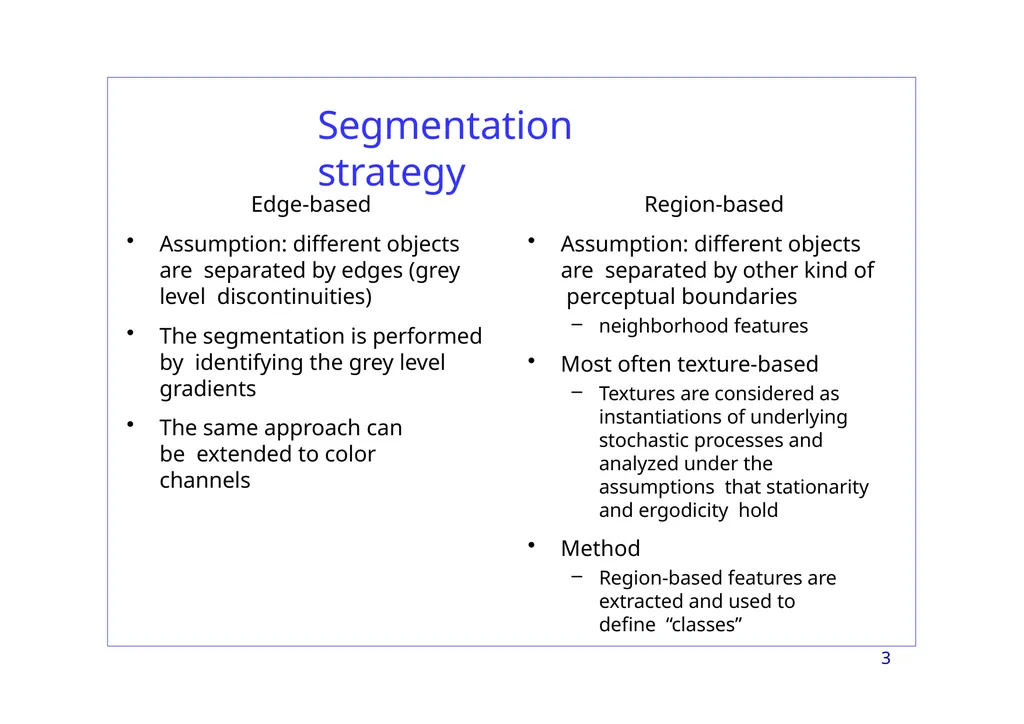
slide3. Segmentation strategy 3 Edge-based
Assumption: different objects are separated by edges (grey level discontinuities)
The segmentation is performed by identifying the grey level gradients
The same approach can be extended to color channels Region-based
Assumption: different objects are separated by other kind of perceptual boundaries
neighborhood features
Most often texture-based
Textures are considered as instantiations of underlying stochastic processes and analyzed under the assumptions that stationarity and ergodicity hold
Method
Region-based features are extracted and used to define “classes”<br>
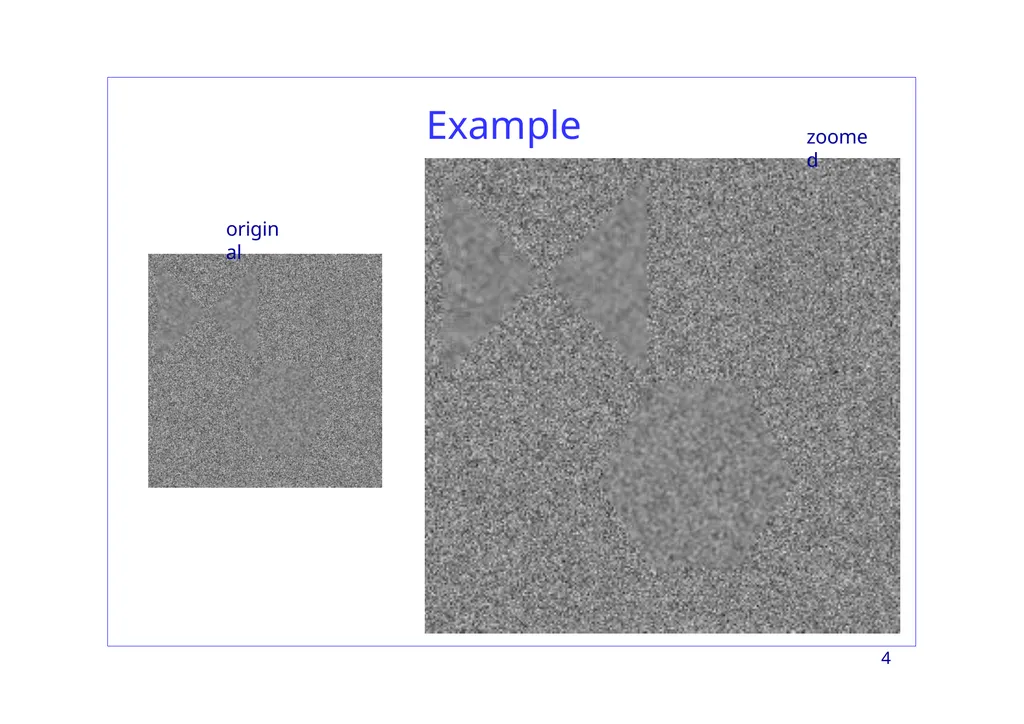
slide4. Examples original 4 zoomed<br>
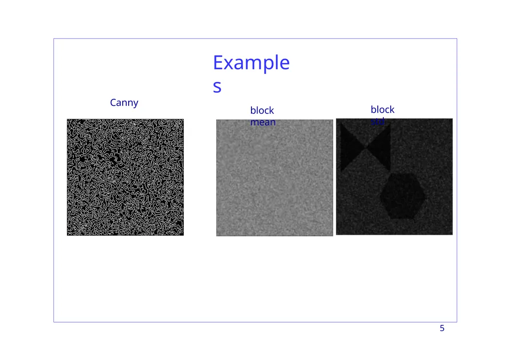
slide5. Examples Canny 5 block mean block std<br>
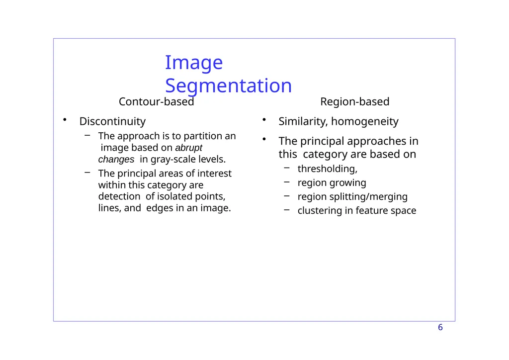
slide6. Image Segmentation 6 Contour-based
Discontinuity
The approach is to partition an image based on abrupt changes in gray-scale levels.
The principal areas of interest within this category are detection of isolated points, lines, and edges in an image. Region-based
Similarity, homogeneity
The principal approaches in this category are based on
thresholding,
region growing
region splitting/merging
clustering in feature space<br>
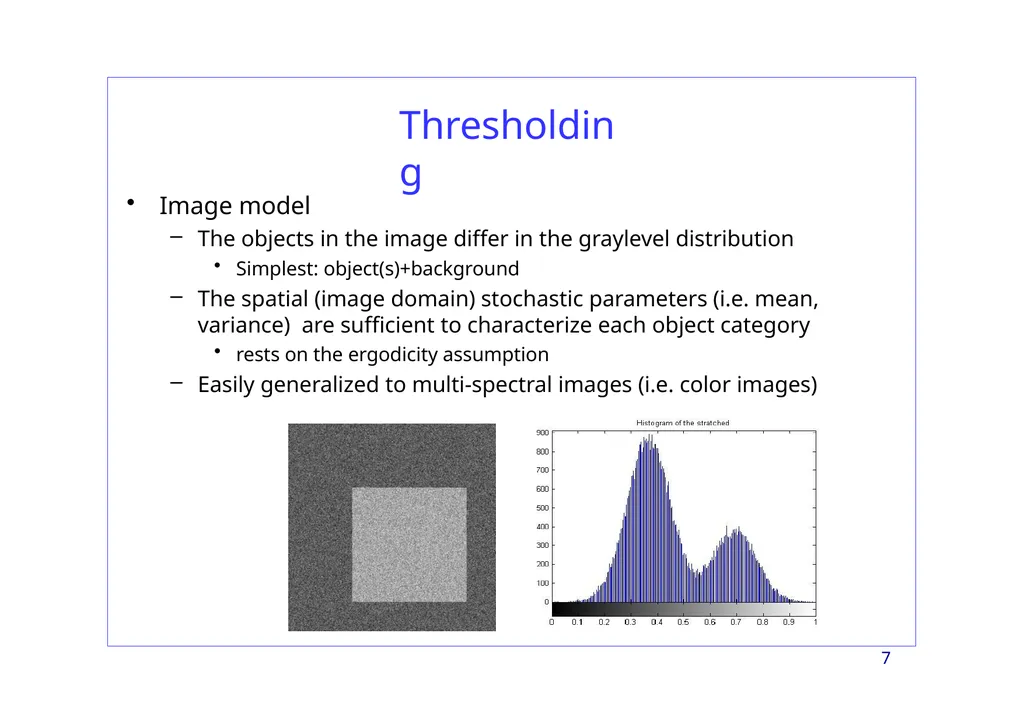
slide7. Thresholding Image model
The objects in the image differ in the graylevel distribution
Simplest: object(s)+background
The spatial (image domain) stochastic parameters (i.e. mean, variance) are sufficient to characterize each object category
rests on the ergodicity assumption
Easily generalized to multi-spectral images (i.e. color images) 7<br>
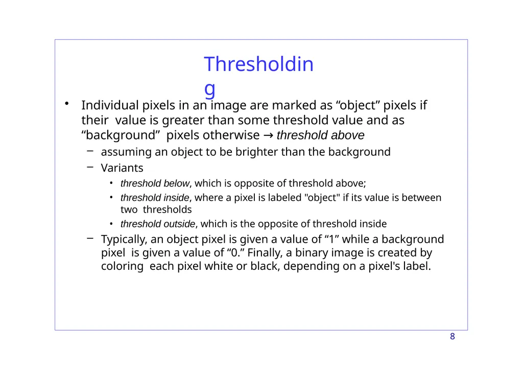
slide8. Thresholding 8 Individual pixels in an image are marked as “object” pixels if their value is greater than some threshold value and as “background” pixels otherwise → threshold above
assuming an object to be brighter than the background
Variants
threshold below, which is opposite of threshold above;
threshold inside, where a pixel is labeled "object" if its value is between two thresholds
threshold outside, which is the opposite of threshold inside
Typically, an object pixel is given a value of “1” while a background pixel is given a value of “0.” Finally, a binary image is created by coloring each pixel white or black, depending on a pixel's label.<br>
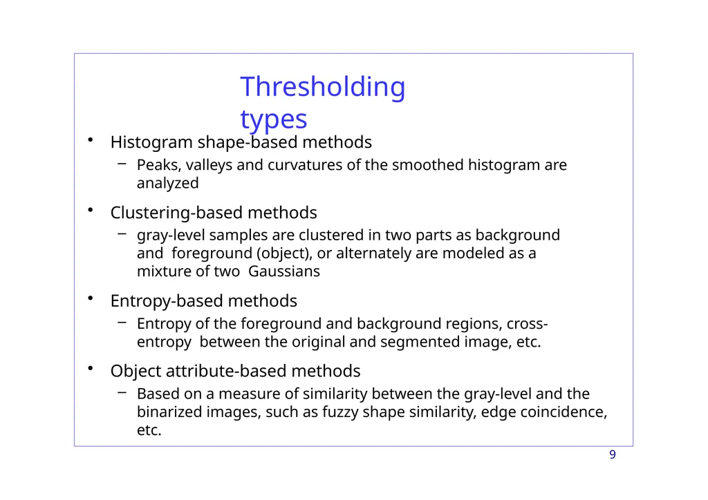
slide9. Thresholding types 9 Histogram shape-based methods
Peaks, valleys and curvatures of the smoothed histogram are analyzed
Clustering-based methods
gray-level samples are clustered in two parts as background and foreground (object), or alternately are modeled as a mixture of two Gaussians
Entropy-based methods
Entropy of the foreground and background regions, cross-entropy between the original and segmented image, etc.
Object attribute-based methods
Based on a measure of similarity between the gray-level and the binarized images, such as fuzzy shape similarity, edge coincidence, etc.<br>
slide10. Thresholding types 10 Stchastic methods using higher-order probability distributions and/or correlation between pixels
Local methods adapt the threshold value on each pixel to the local image characteristics<br>
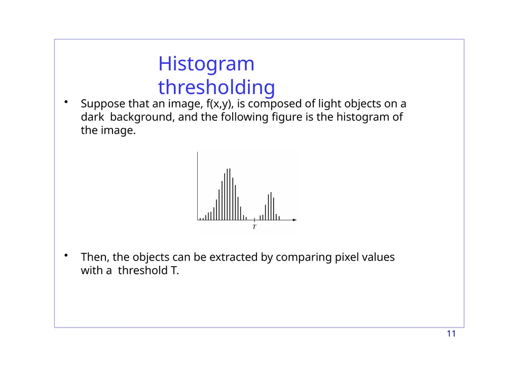
slide11. Histogram thresholding Suppose that an image, f(x,y), is composed of light objects on a dark background, and the following figure is the histogram of the image. Then, the objects can be extracted by comparing pixel values with a threshold T. 11<br>
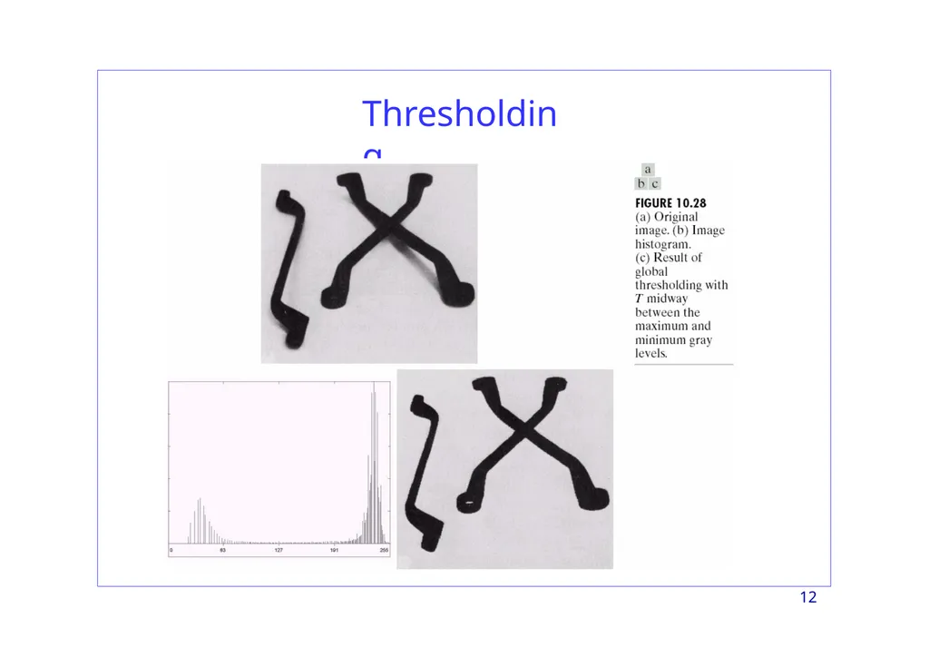
slide12. Thresholding 12<br>
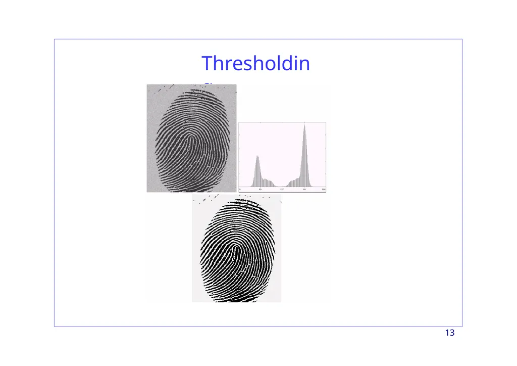
slide13. Thresholding 13<br>
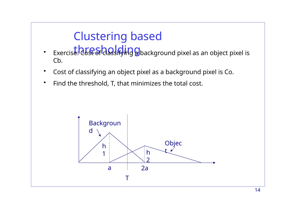
slide14. Clustering based thresholding Exercise: Cost of classifying a background pixel as an object pixel is Cb.
Cost of classifying an object pixel as a background pixel is Co.
Find the threshold, T, that minimizes the total cost. a 2a h1 h2 T Background Object 14<br>
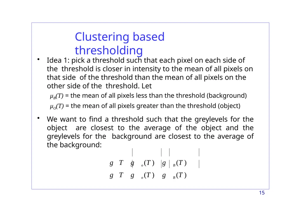
slide15. Clustering based thresholding Idea 1: pick a threshold such that each pixel on each side of the threshold is closer in intensity to the mean of all pixels on that side of the threshold than the mean of all pixels on the other side of the threshold. Let
μB(T) = the mean of all pixels less than the threshold (background)
μO(T) = the mean of all pixels greater than the threshold (object)
We want to find a threshold such that the greylevels for the object are closest to the average of the object and the greylevels for the background are closest to the average of the background:
g T g o (T ) g B (T )
g T g o (T ) g B (T ) 15<br>
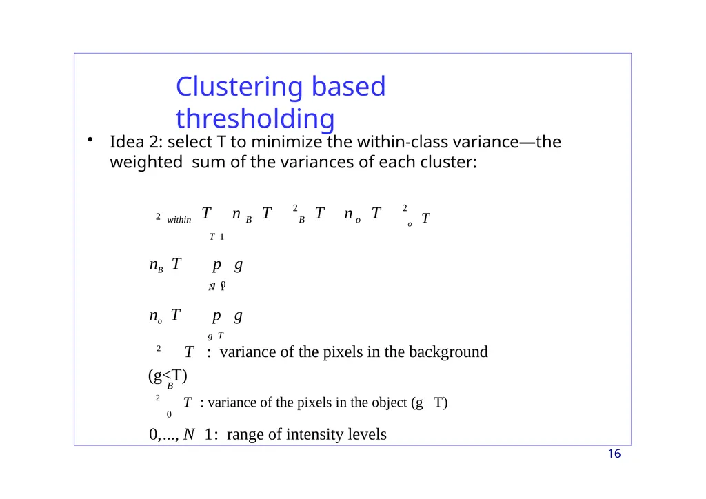
slide16. Clustering based thresholding 16 Idea 2: select T to minimize the within-class variance—the weighted sum of the variances of each cluster: 2 2 within B B o o T 2 T 1 N 1 T n T T n T nB T p g
g 0 no T p g
g T
2 T : variance of the pixels in the background (g<T)
B
2 T : variance of the pixels in the object (g T)
0
0,..., N 1: range of intensity levels<br>
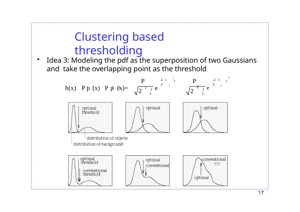
slide17. Clustering based thresholding Idea 3: Modeling the pdf as the superposition of two Gaussians and take the overlapping point as the threshold 1 1 2 2 2
1 2
2 P P 2 2 1 x 2 1 x 2 1 2 2 1 2 2 h(x) P p (x) P p (x)= 1 e 2 e 17<br>
slide18. Thresholding 18 Non-uniform illumination may change the histogram in a way that it becomes impossible to segment the image using a single global threshold.
Choosing local threshold values may help.<br>
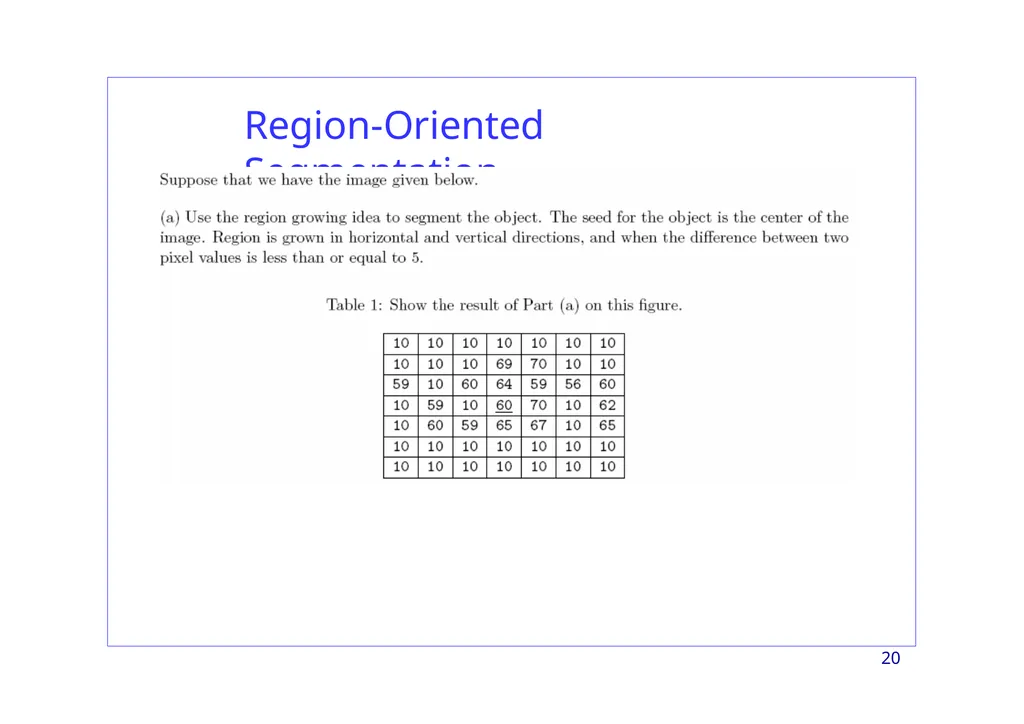
slide19. Region-Oriented Segmentation 19 Region Growing
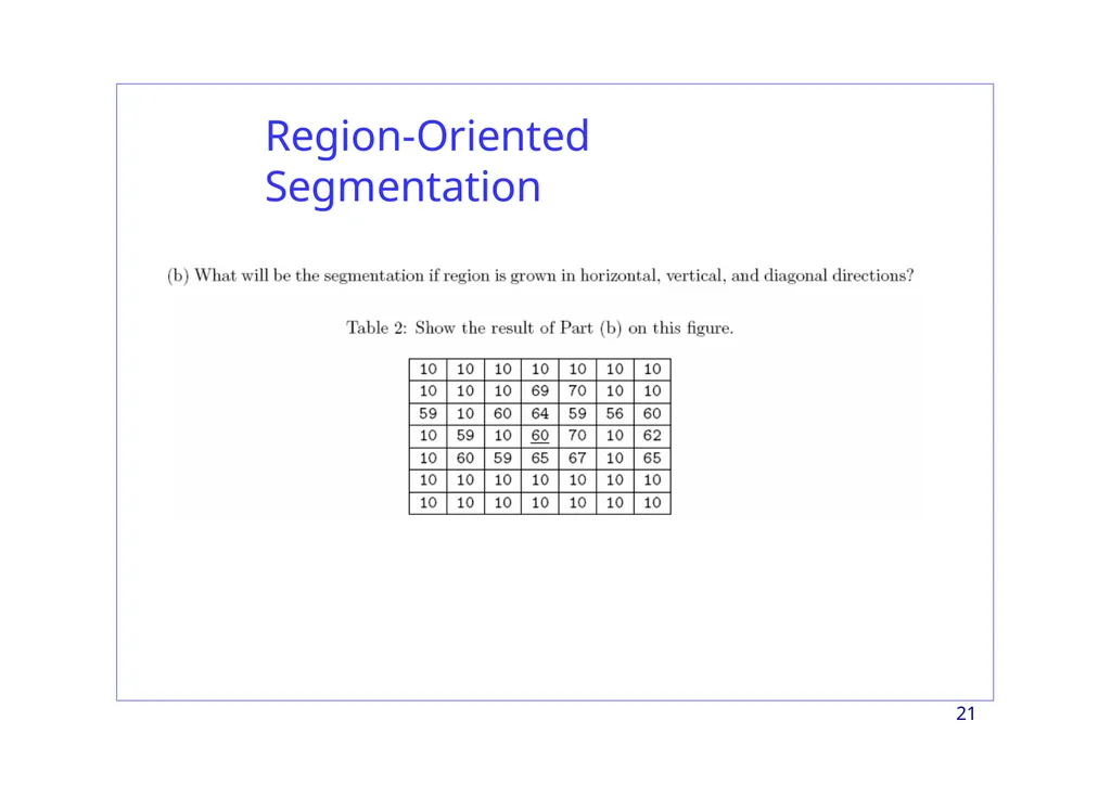
Region growing is a procedure that groups pixels or subregions into larger regions.
The simplest of these approaches is pixel aggregation, which starts with a set of “seed” points and from these grows regions by appending to each seed points those neighboring pixels that have similar properties (such as gray level, texture, color, shape).
Region growing based techniques are better than the edge-based techniques in noisy images where edges are difficult to detect.<br>
slide20. Region-Oriented Segmentation 20<br>
slide21. Region-Oriented Segmentation 21<br>
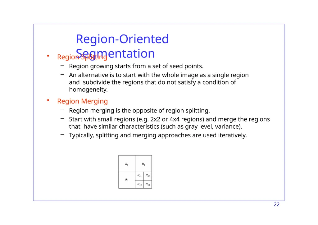
slide22. Region-Oriented Segmentation Region Splitting
Region growing starts from a set of seed points.
An alternative is to start with the whole image as a single region and subdivide the regions that do not satisfy a condition of homogeneity.
Region Merging
Region merging is the opposite of region splitting.
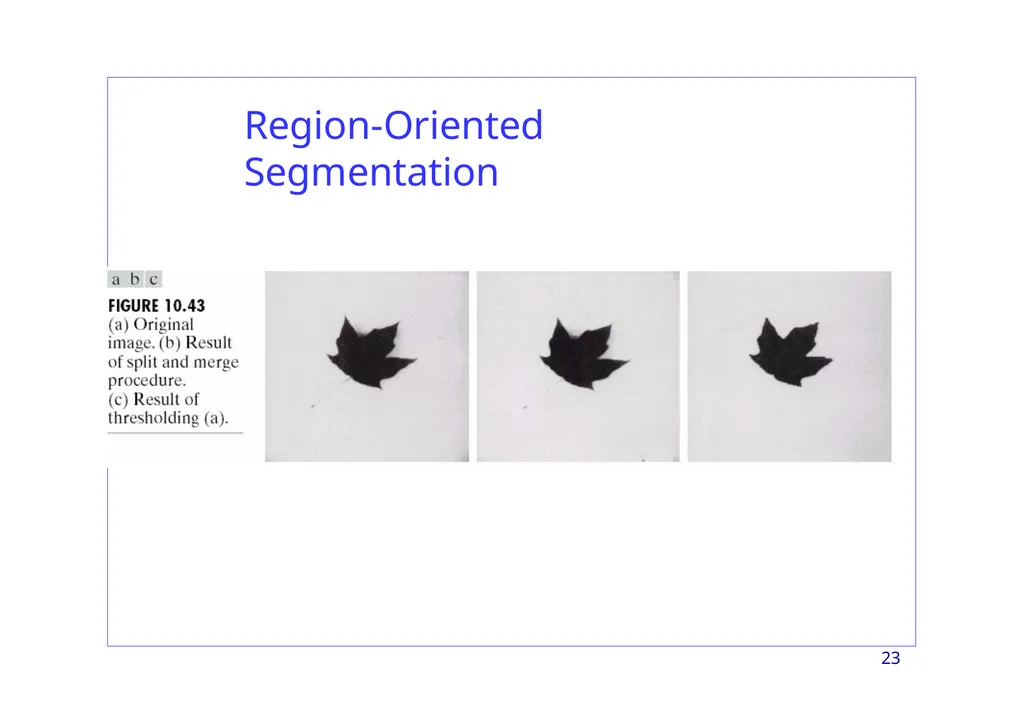
Start with small regions (e.g. 2x2 or 4x4 regions) and merge the regions that have similar characteristics (such as gray level, variance).
Typically, splitting and merging approaches are used iteratively. 22<br>
slide23. Region-Oriented Segmentation 23<br>
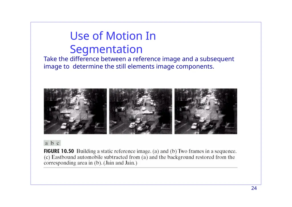
slide24. Take the difference between a reference image and a subsequent image to determine the still elements image components. Use of Motion In Segmentation 24<br>
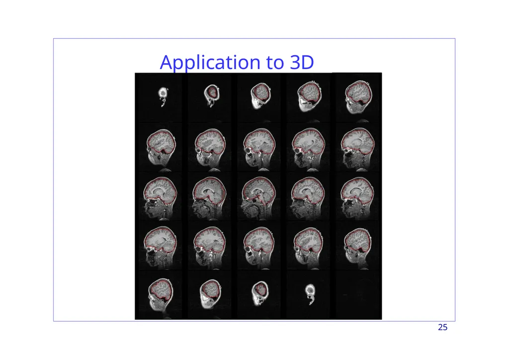
slide25. Application to 3D data 25<br>
slide26. Clustering and Classification<br>
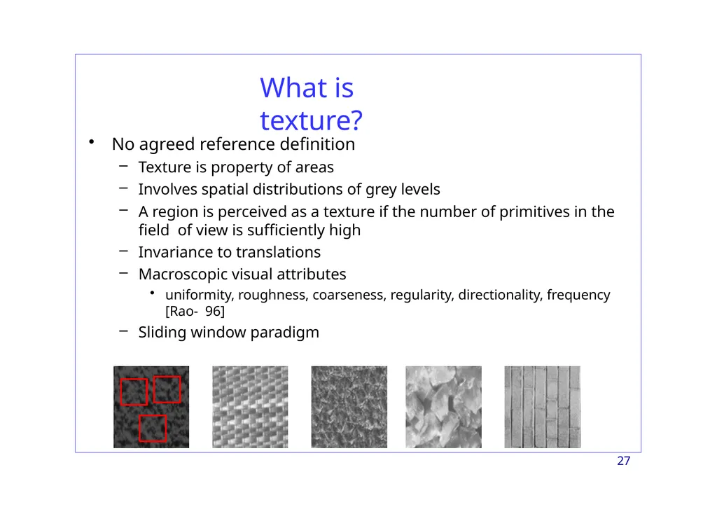
slide27. What is texture? No agreed reference definition
Texture is property of areas
Involves spatial distributions of grey levels
A region is perceived as a texture if the number of primitives in the field of view is sufficiently high
Invariance to translations
Macroscopic visual attributes
uniformity, roughness, coarseness, regularity, directionality, frequency [Rao- 96]
Sliding window paradigm 27<br>
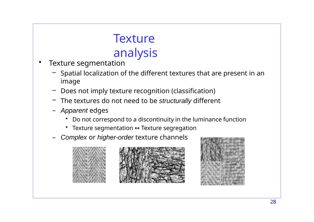
slide28. Texture analysis Texture segmentation
Spatial localization of the different textures that are present in an image
Does not imply texture recognition (classification)
The textures do not need to be structurally different
Apparent edges
Do not correspond to a discontinuity in the luminance function
Texture segmentation ↔ Texture segregation
Complex or higher-order texture channels 28<br>
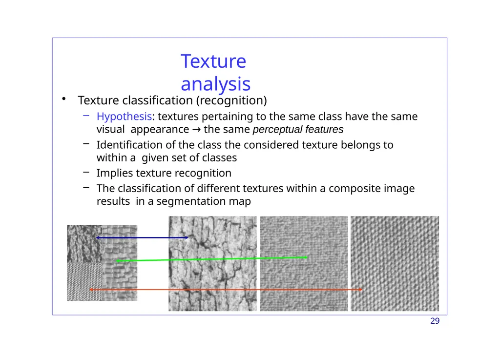
slide29. Texture analysis Texture classification (recognition)
Hypothesis: textures pertaining to the same class have the same visual appearance → the same perceptual features
Identification of the class the considered texture belongs to within a given set of classes
Implies texture recognition
The classification of different textures within a composite image results in a segmentation map 29<br>
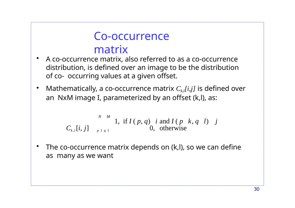
slide30. Co-occurrence matrix 30 A co-occurrence matrix, also referred to as a co-occurrence distribution, is defined over an image to be the distribution of co- occurring values at a given offset.
Mathematically, a co-occurrence matrix Ck,l[i,j] is defined over an NxM image I, parameterized by an offset (k,l), as: The co-occurrence matrix depends on (k,l), so we can define as many as we want 0, otherwise N M 1, if I ( p, q) i and I ( p k, q l) j p 1 q 1 Ck ,l [i, j] <br>
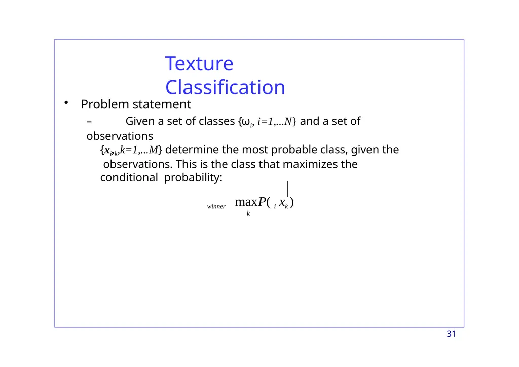
slide31. Texture Classification Problem statement
– Given a set of classes {ωi, i=1,...N} and a set of observations
{xi,k,k=1,...M} determine the most probable class, given the observations. This is the class that maximizes the conditional probability:
winner maxP(i xk )
k 31<br>
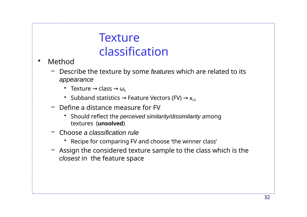
slide32. Texture classification 32 Method
Describe the texture by some features which are related to its
appearance
Texture → class → ωk
Subband statistics → Feature Vectors (FV) → xi,k
Define a distance measure for FV
Should reflect the perceived similarity/dissimilarity among textures (unsolved)
Choose a classification rule
Recipe for comparing FV and choose ‘the winner class’
Assign the considered texture sample to the class which is the closest in the feature space<br>
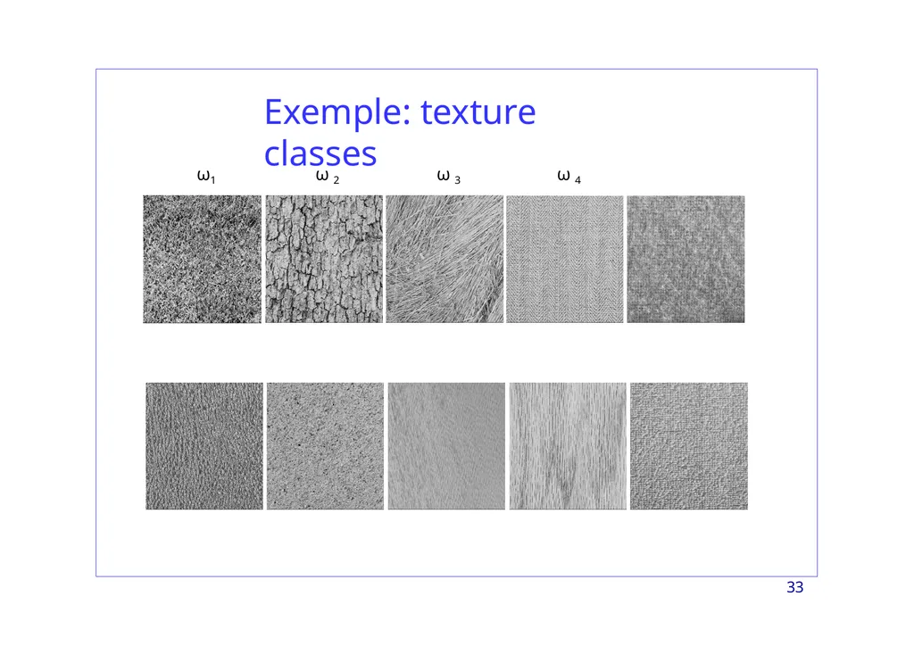
slide33. Exemple: texture classes ω1 33 ω 2 ω 3 ω 4<br>
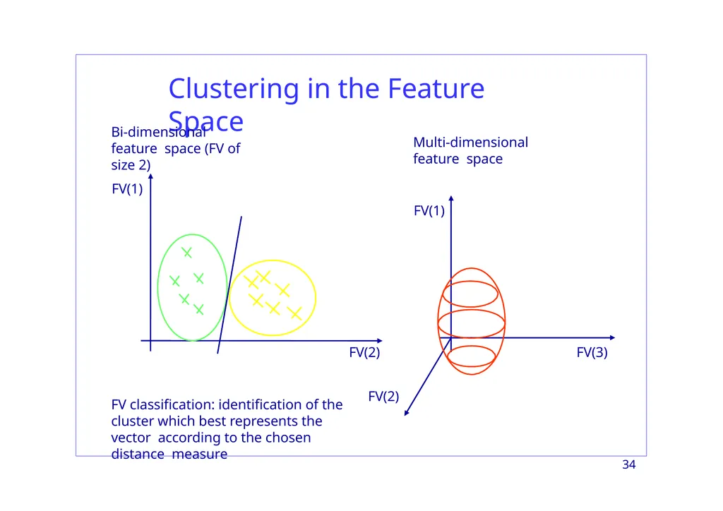
slide34. Clustering in the Feature Space Bi-dimensional feature space (FV of size 2) FV(1) FV(2) FV(3) 34 FV(2) FV(1) Multi-dimensional feature space FV classification: identification of the cluster which best represents the vector according to the chosen distance measure<br>
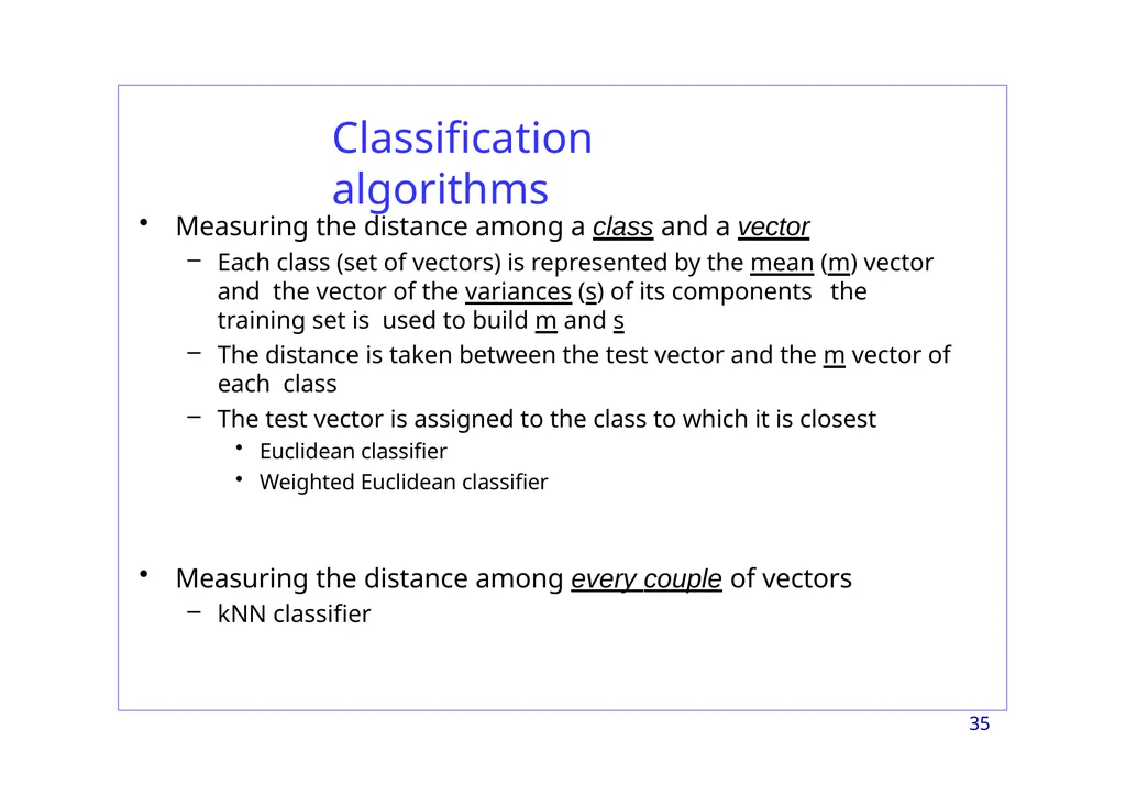
slide35. Classification algorithms 35 Measuring the distance among a class and a vector
Each class (set of vectors) is represented by the mean (m) vector and the vector of the variances (s) of its components the training set is used to build m and s
The distance is taken between the test vector and the m vector of each class
The test vector is assigned to the class to which it is closest
Euclidean classifier
Weighted Euclidean classifier
Measuring the distance among every couple of vectors
kNN classifier<br>
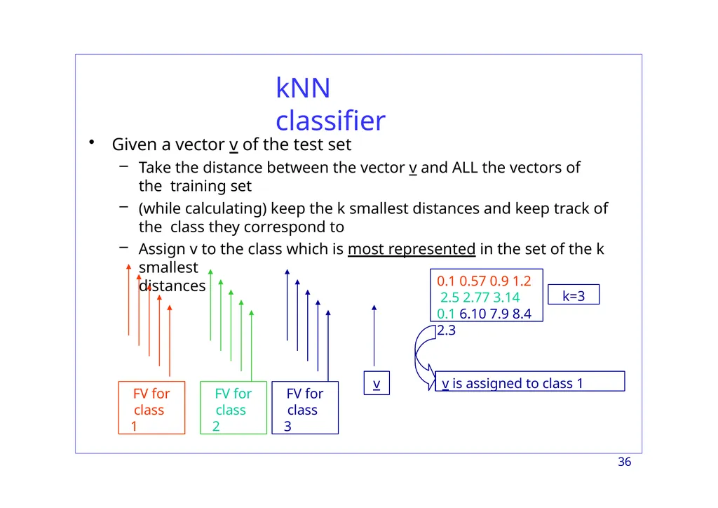
slide36. kNN classifier Given a vector v of the test set
Take the distance between the vector v and ALL the vectors of the training set
(while calculating) keep the k smallest distances and keep track of the class they correspond to
Assign v to the class which is most represented in the set of the k smallest distances FV for class 1 FV for class 2 FV for class 3 v 0.1 0.57 0.9 1.2 2.5 2.77 3.14 0.1 6.10 7.9 8.4 2.3 k=3 v is assigned to class 1 36<br>
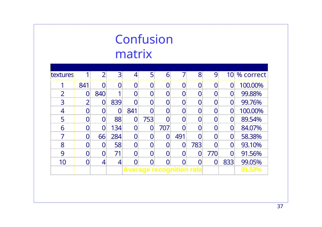
slide37. Confusion matrix 37<br>
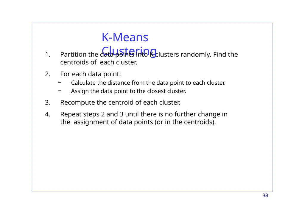
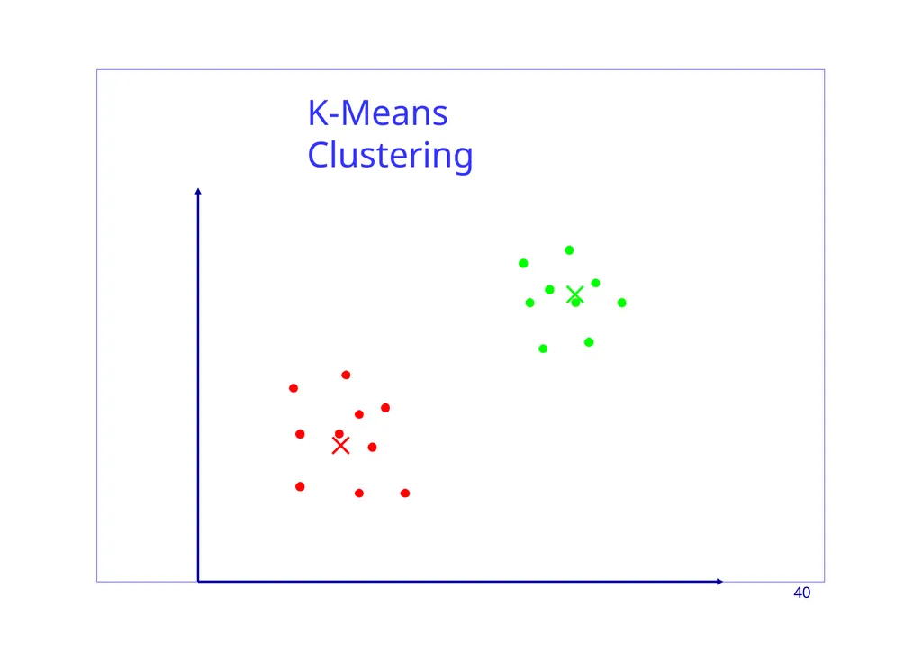
slide38. K-Means Clustering 38 Partition the data points into K clusters randomly. Find the centroids of each cluster.
For each data point:
Calculate the distance from the data point to each cluster.
Assign the data point to the closest cluster.
Recompute the centroid of each cluster.
Repeat steps 2 and 3 until there is no further change in the assignment of data points (or in the centroids).<br>
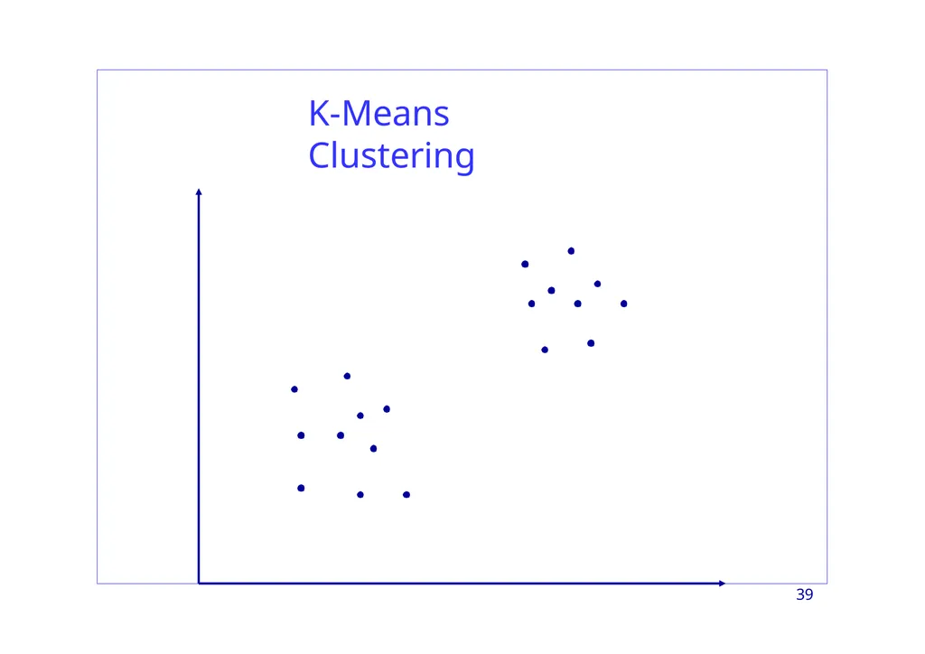
slide39. K-Means Clustering 39<br>
slide40. K-Means Clustering 40<br>
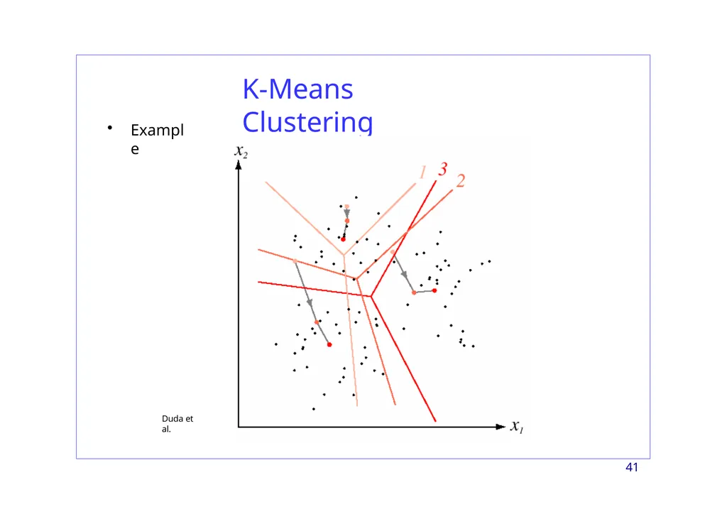
slide41. K-Means Clustering Example Duda et al. 41<br>
slide2. Image Segmentation 2 Group similar components (such as, pixels in an image, image frames in a video) to obtain a compact representation.
Applications: Finding tumors, veins, etc. in medical images, finding targets in satellite/aerial images, finding people in surveillance images, summarizing video, etc.
Methods: Thresholding, K-means clustering, etc.<br>
slide3. Segmentation strategy 3 Edge-based
Assumption: different objects are separated by edges (grey level discontinuities)
The segmentation is performed by identifying the grey level gradients
The same approach can be extended to color channels Region-based
Assumption: different objects are separated by other kind of perceptual boundaries
neighborhood features
Most often texture-based
Textures are considered as instantiations of underlying stochastic processes and analyzed under the assumptions that stationarity and ergodicity hold
Method
Region-based features are extracted and used to define “classes”<br>
slide4. Examples original 4 zoomed<br>
slide5. Examples Canny 5 block mean block std<br>
slide6. Image Segmentation 6 Contour-based
Discontinuity
The approach is to partition an image based on abrupt changes in gray-scale levels.
The principal areas of interest within this category are detection of isolated points, lines, and edges in an image. Region-based
Similarity, homogeneity
The principal approaches in this category are based on
thresholding,
region growing
region splitting/merging
clustering in feature space<br>
slide7. Thresholding Image model
The objects in the image differ in the graylevel distribution
Simplest: object(s)+background
The spatial (image domain) stochastic parameters (i.e. mean, variance) are sufficient to characterize each object category
rests on the ergodicity assumption
Easily generalized to multi-spectral images (i.e. color images) 7<br>
slide8. Thresholding 8 Individual pixels in an image are marked as “object” pixels if their value is greater than some threshold value and as “background” pixels otherwise → threshold above
assuming an object to be brighter than the background
Variants
threshold below, which is opposite of threshold above;
threshold inside, where a pixel is labeled "object" if its value is between two thresholds
threshold outside, which is the opposite of threshold inside
Typically, an object pixel is given a value of “1” while a background pixel is given a value of “0.” Finally, a binary image is created by coloring each pixel white or black, depending on a pixel's label.<br>
slide9. Thresholding types 9 Histogram shape-based methods
Peaks, valleys and curvatures of the smoothed histogram are analyzed
Clustering-based methods
gray-level samples are clustered in two parts as background and foreground (object), or alternately are modeled as a mixture of two Gaussians
Entropy-based methods
Entropy of the foreground and background regions, cross-entropy between the original and segmented image, etc.
Object attribute-based methods
Based on a measure of similarity between the gray-level and the binarized images, such as fuzzy shape similarity, edge coincidence, etc.<br>
slide10. Thresholding types 10 Stchastic methods using higher-order probability distributions and/or correlation between pixels
Local methods adapt the threshold value on each pixel to the local image characteristics<br>
slide11. Histogram thresholding Suppose that an image, f(x,y), is composed of light objects on a dark background, and the following figure is the histogram of the image. Then, the objects can be extracted by comparing pixel values with a threshold T. 11<br>
slide12. Thresholding 12<br>
slide13. Thresholding 13<br>
slide14. Clustering based thresholding Exercise: Cost of classifying a background pixel as an object pixel is Cb.
Cost of classifying an object pixel as a background pixel is Co.
Find the threshold, T, that minimizes the total cost. a 2a h1 h2 T Background Object 14<br>
slide15. Clustering based thresholding Idea 1: pick a threshold such that each pixel on each side of the threshold is closer in intensity to the mean of all pixels on that side of the threshold than the mean of all pixels on the other side of the threshold. Let
μB(T) = the mean of all pixels less than the threshold (background)
μO(T) = the mean of all pixels greater than the threshold (object)
We want to find a threshold such that the greylevels for the object are closest to the average of the object and the greylevels for the background are closest to the average of the background:
g T g o (T ) g B (T )
g T g o (T ) g B (T ) 15<br>
slide16. Clustering based thresholding 16 Idea 2: select T to minimize the within-class variance—the weighted sum of the variances of each cluster: 2 2 within B B o o T 2 T 1 N 1 T n T T n T nB T p g
g 0 no T p g
g T
2 T : variance of the pixels in the background (g<T)
B
2 T : variance of the pixels in the object (g T)
0
0,..., N 1: range of intensity levels<br>
slide17. Clustering based thresholding Idea 3: Modeling the pdf as the superposition of two Gaussians and take the overlapping point as the threshold 1 1 2 2 2
1 2
2 P P 2 2 1 x 2 1 x 2 1 2 2 1 2 2 h(x) P p (x) P p (x)= 1 e 2 e 17<br>
slide18. Thresholding 18 Non-uniform illumination may change the histogram in a way that it becomes impossible to segment the image using a single global threshold.
Choosing local threshold values may help.<br>
slide19. Region-Oriented Segmentation 19 Region Growing
Region growing is a procedure that groups pixels or subregions into larger regions.
The simplest of these approaches is pixel aggregation, which starts with a set of “seed” points and from these grows regions by appending to each seed points those neighboring pixels that have similar properties (such as gray level, texture, color, shape).
Region growing based techniques are better than the edge-based techniques in noisy images where edges are difficult to detect.<br>
slide20. Region-Oriented Segmentation 20<br>
slide21. Region-Oriented Segmentation 21<br>
slide22. Region-Oriented Segmentation Region Splitting
Region growing starts from a set of seed points.
An alternative is to start with the whole image as a single region and subdivide the regions that do not satisfy a condition of homogeneity.
Region Merging
Region merging is the opposite of region splitting.
Start with small regions (e.g. 2x2 or 4x4 regions) and merge the regions that have similar characteristics (such as gray level, variance).
Typically, splitting and merging approaches are used iteratively. 22<br>
slide23. Region-Oriented Segmentation 23<br>
slide24. Take the difference between a reference image and a subsequent image to determine the still elements image components. Use of Motion In Segmentation 24<br>
slide25. Application to 3D data 25<br>
slide26. Clustering and Classification<br>
slide27. What is texture? No agreed reference definition
Texture is property of areas
Involves spatial distributions of grey levels
A region is perceived as a texture if the number of primitives in the field of view is sufficiently high
Invariance to translations
Macroscopic visual attributes
uniformity, roughness, coarseness, regularity, directionality, frequency [Rao- 96]
Sliding window paradigm 27<br>
slide28. Texture analysis Texture segmentation
Spatial localization of the different textures that are present in an image
Does not imply texture recognition (classification)
The textures do not need to be structurally different
Apparent edges
Do not correspond to a discontinuity in the luminance function
Texture segmentation ↔ Texture segregation
Complex or higher-order texture channels 28<br>
slide29. Texture analysis Texture classification (recognition)
Hypothesis: textures pertaining to the same class have the same visual appearance → the same perceptual features
Identification of the class the considered texture belongs to within a given set of classes
Implies texture recognition
The classification of different textures within a composite image results in a segmentation map 29<br>
slide30. Co-occurrence matrix 30 A co-occurrence matrix, also referred to as a co-occurrence distribution, is defined over an image to be the distribution of co- occurring values at a given offset.
Mathematically, a co-occurrence matrix Ck,l[i,j] is defined over an NxM image I, parameterized by an offset (k,l), as: The co-occurrence matrix depends on (k,l), so we can define as many as we want 0, otherwise N M 1, if I ( p, q) i and I ( p k, q l) j p 1 q 1 Ck ,l [i, j] <br>
slide31. Texture Classification Problem statement
– Given a set of classes {ωi, i=1,...N} and a set of observations
{xi,k,k=1,...M} determine the most probable class, given the observations. This is the class that maximizes the conditional probability:
winner maxP(i xk )
k 31<br>
slide32. Texture classification 32 Method
Describe the texture by some features which are related to its
appearance
Texture → class → ωk
Subband statistics → Feature Vectors (FV) → xi,k
Define a distance measure for FV
Should reflect the perceived similarity/dissimilarity among textures (unsolved)
Choose a classification rule
Recipe for comparing FV and choose ‘the winner class’
Assign the considered texture sample to the class which is the closest in the feature space<br>
slide33. Exemple: texture classes ω1 33 ω 2 ω 3 ω 4<br>
slide34. Clustering in the Feature Space Bi-dimensional feature space (FV of size 2) FV(1) FV(2) FV(3) 34 FV(2) FV(1) Multi-dimensional feature space FV classification: identification of the cluster which best represents the vector according to the chosen distance measure<br>
slide35. Classification algorithms 35 Measuring the distance among a class and a vector
Each class (set of vectors) is represented by the mean (m) vector and the vector of the variances (s) of its components the training set is used to build m and s
The distance is taken between the test vector and the m vector of each class
The test vector is assigned to the class to which it is closest
Euclidean classifier
Weighted Euclidean classifier
Measuring the distance among every couple of vectors
kNN classifier<br>
slide36. kNN classifier Given a vector v of the test set
Take the distance between the vector v and ALL the vectors of the training set
(while calculating) keep the k smallest distances and keep track of the class they correspond to
Assign v to the class which is most represented in the set of the k smallest distances FV for class 1 FV for class 2 FV for class 3 v 0.1 0.57 0.9 1.2 2.5 2.77 3.14 0.1 6.10 7.9 8.4 2.3 k=3 v is assigned to class 1 36<br>
slide37. Confusion matrix 37<br>
slide38. K-Means Clustering 38 Partition the data points into K clusters randomly. Find the centroids of each cluster.
For each data point:
Calculate the distance from the data point to each cluster.
Assign the data point to the closest cluster.
Recompute the centroid of each cluster.
Repeat steps 2 and 3 until there is no further change in the assignment of data points (or in the centroids).<br>
slide39. K-Means Clustering 39<br>
slide40. K-Means Clustering 40<br>
slide41. K-Means Clustering Example Duda et al. 41<br>