
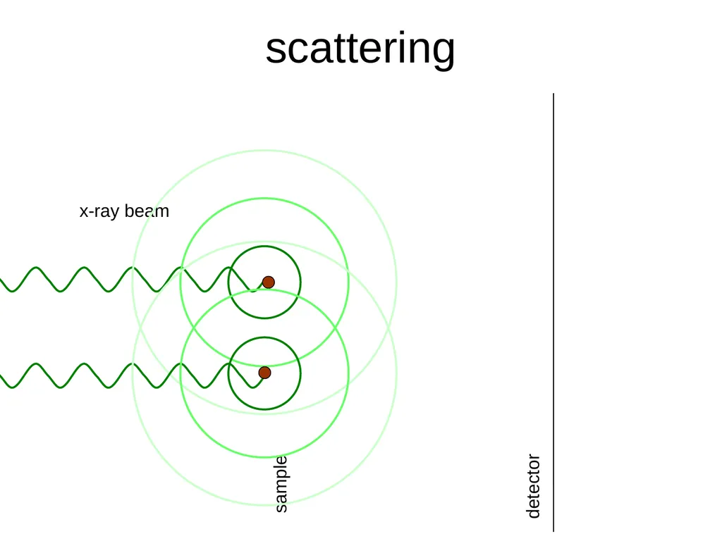
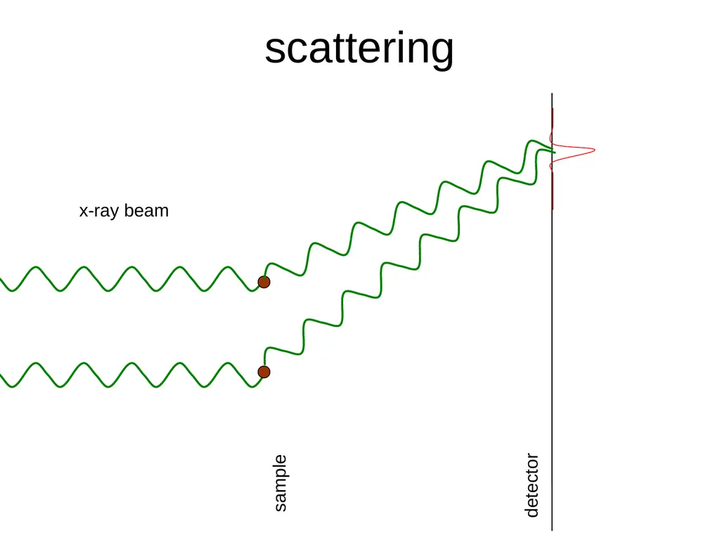
sample x-ray beam scattering sample detector x-ray
LV
Published · 48 slides · 0 views
1 / 1




Description
sample x-ray beam scattering sample detector x-ray beam scattering sample detector x-ray beam scattering sample detector x-ray beam scattering Braggs Law nλ 2d sin(θ) to source d dsin(θ) θ atom 1 atom 2 Braggs Law nλ 2d sin(θ)
Related Topics
Share
Embed code
Download this presentation From Below
"sample x-ray beam scattering sample detector x-ray" is the property of its rightful owner. Permission is granted to download and print the materials on this website for personal, non-commercial use only, and to display it on your personal computer provided you do not modify the materials and that you retain all copyright notices contained in the materials. By downloading content from our website, you accept the terms of this agreement.
Presentation Transcript
01
sample x-ray beam scattering<br>
02
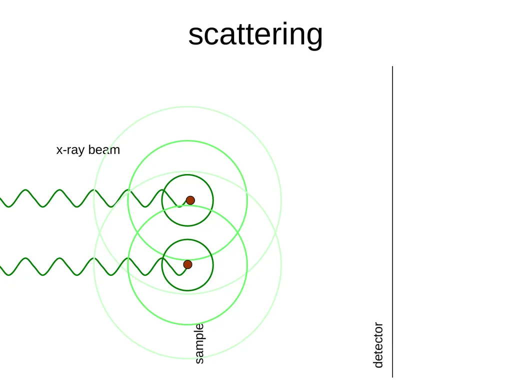
sample detector x-ray beam scattering<br>
03
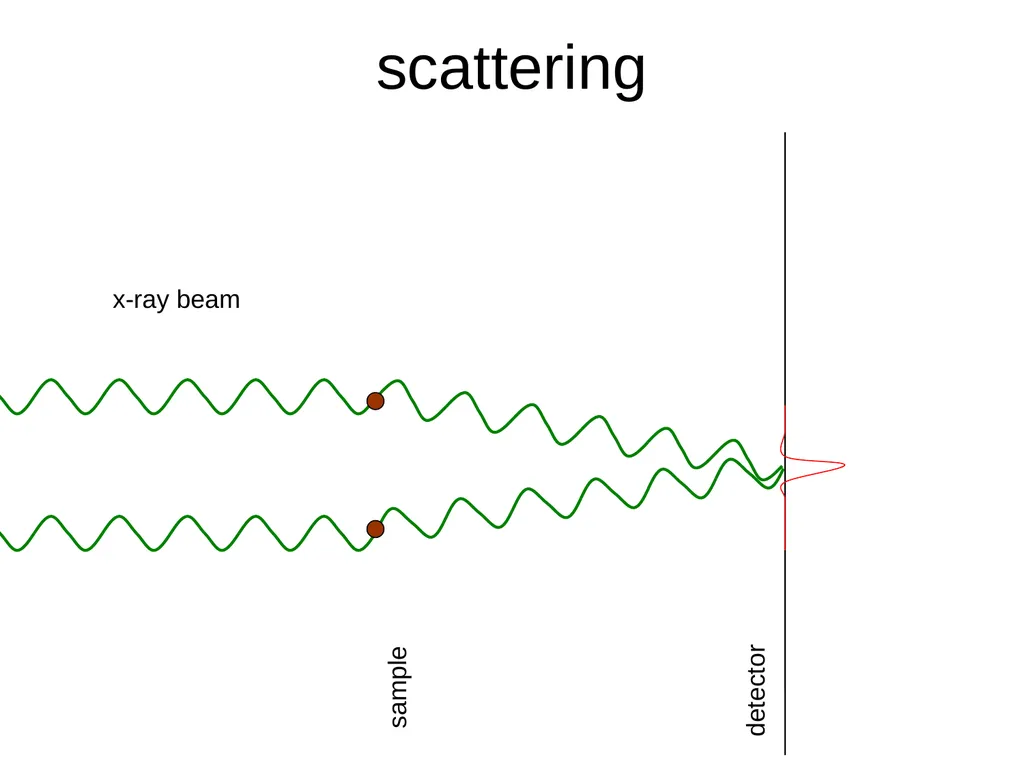
sample detector x-ray beam scattering<br>
04
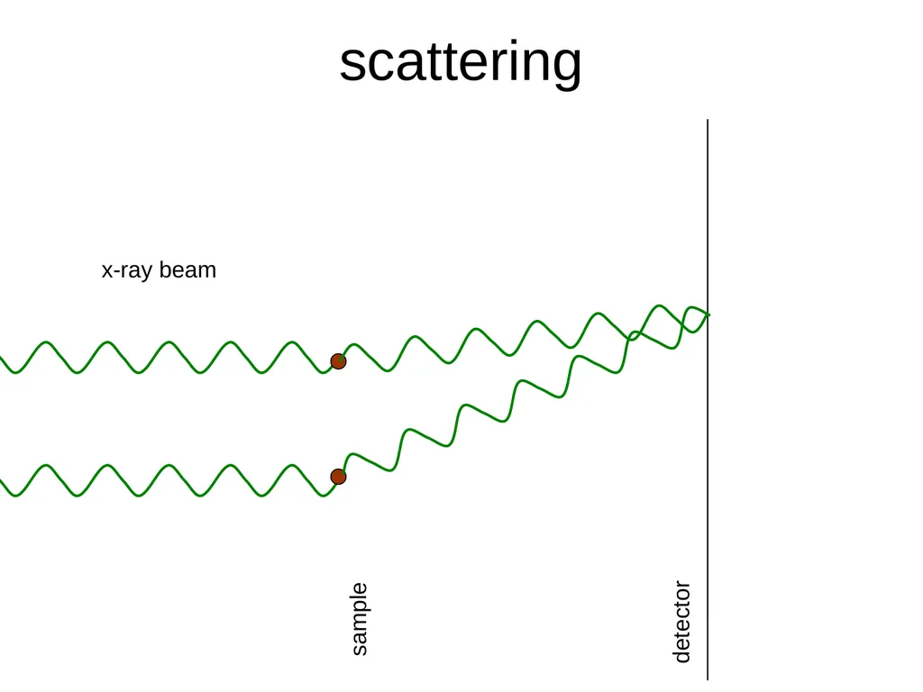
sample detector x-ray beam scattering<br>
05
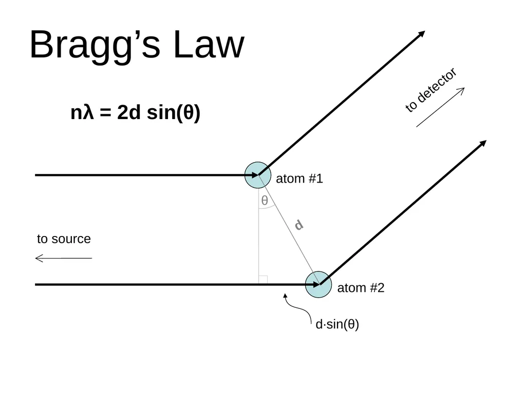
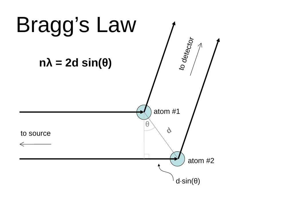
Bragg’s Law nλ = 2d sin(θ)<br>
06
to source d d∙sin(θ) θ atom #1 atom #2 Bragg’s Law nλ = 2d sin(θ)<br>
07
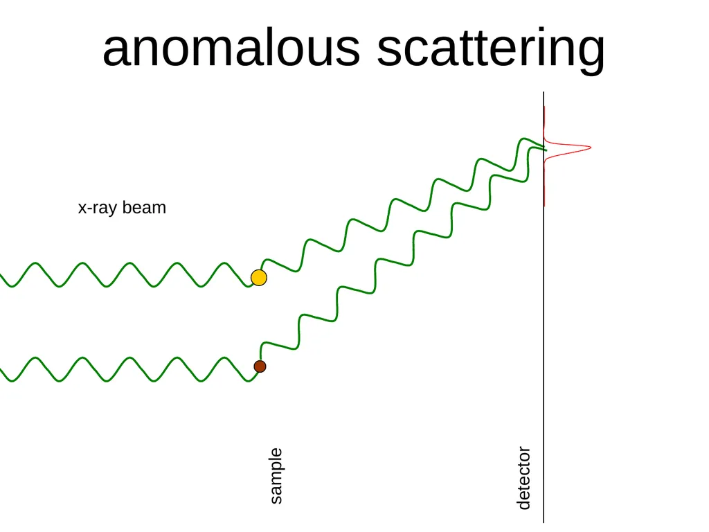
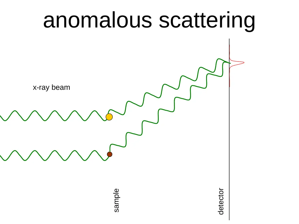
sample x-ray beam anomalous scattering<br>
08
sample detector x-ray beam anomalous scattering<br>
09
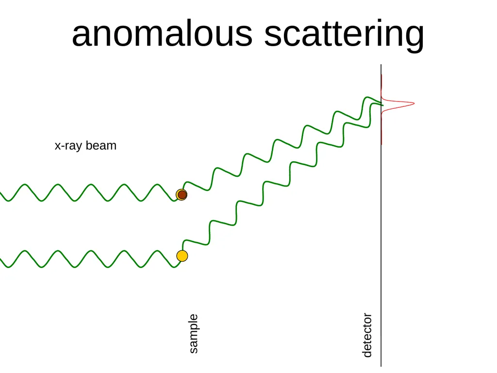
sample x-ray beam anomalous scattering<br>
10
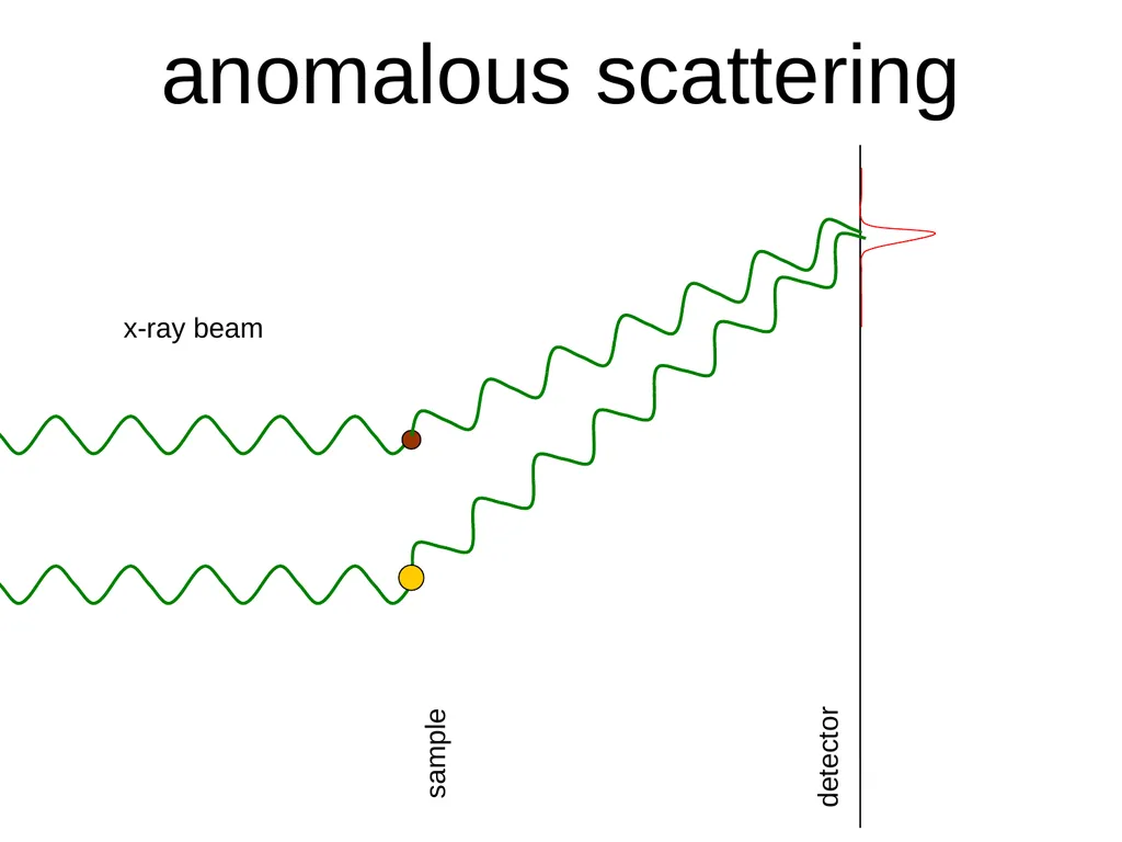
sample detector x-ray beam anomalous scattering<br>
11
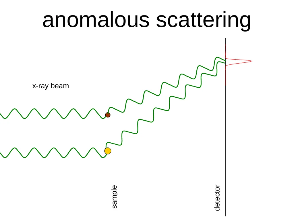
sample detector x-ray beam anomalous scattering<br>
12
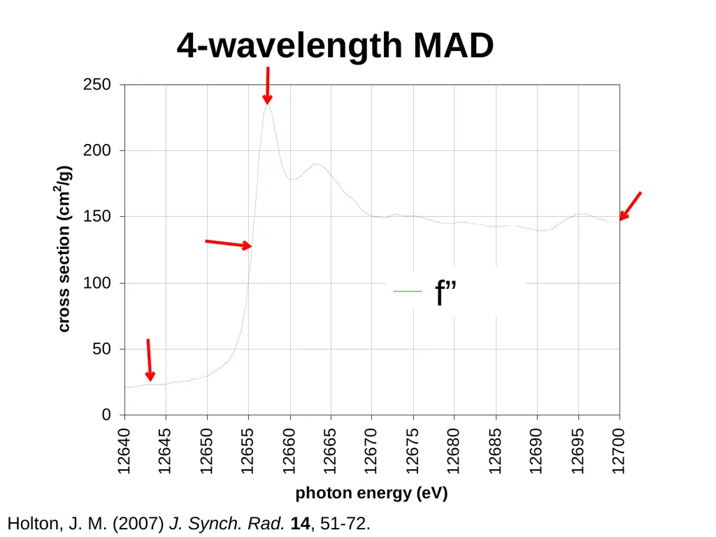
Holton, J. M. (2007) J. Synch. Rad. 14, 51-72. 4-wavelength MAD f”<br>
13
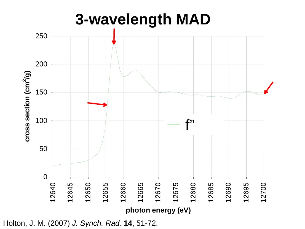
Holton, J. M. (2007) J. Synch. Rad. 14, 51-72. 3-wavelength MAD f”<br>
14
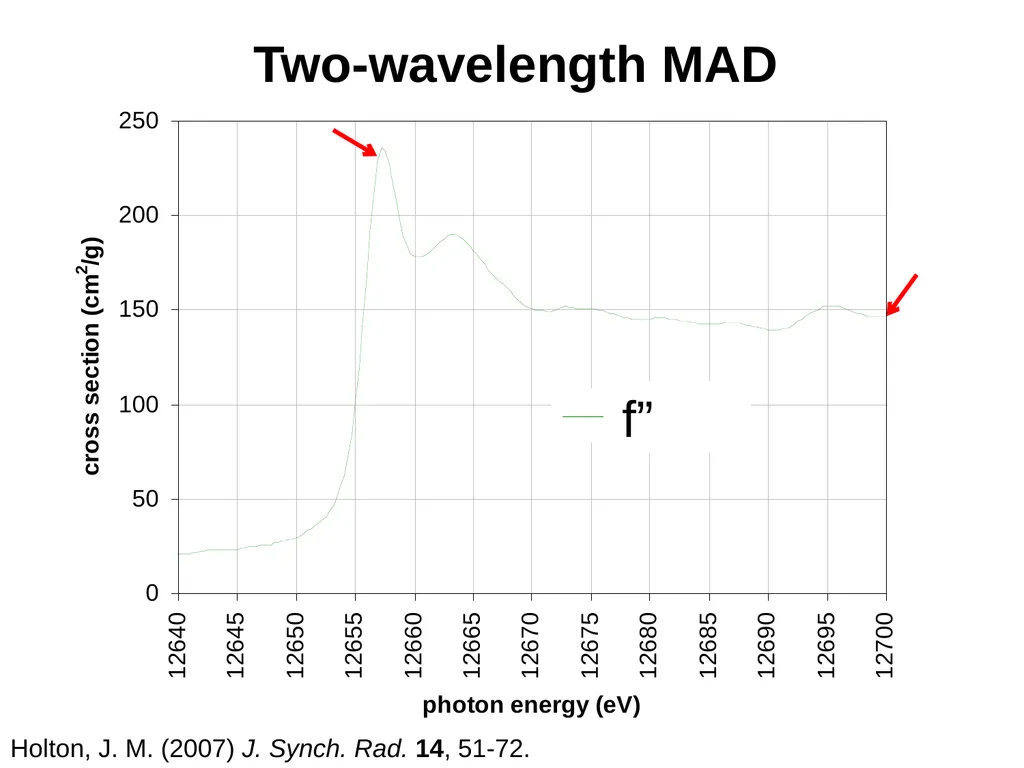
Holton, J. M. (2007) J. Synch. Rad. 14, 51-72. Two-wavelength MAD f”<br>
15
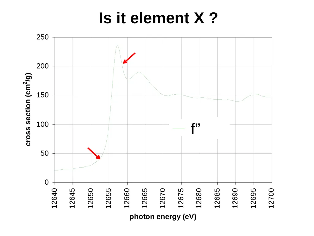
Is it element X ? f”<br>
16
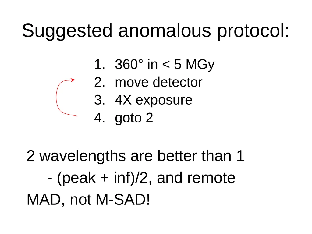
Suggested anomalous protocol: 2 wavelengths are better than 1
- (peak + inf)/2, and remote
MAD, not M-SAD! 360° in < 5 MGy
move detector
4X exposure
goto 2<br>
- (peak + inf)/2, and remote
MAD, not M-SAD! 360° in < 5 MGy
move detector
4X exposure
goto 2<br>
17
Required signal-to-noise (I/σ) Solve-able proteins (%) Phasing from native elements<br>
18
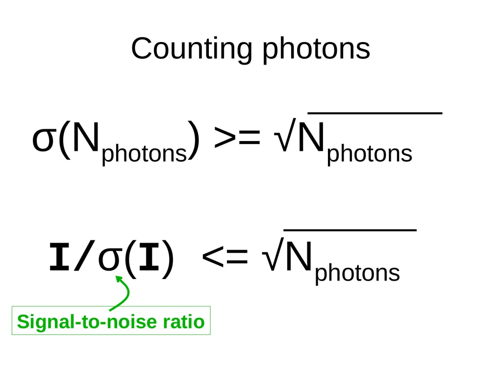
Counting photons σ(Nphotons) >= √Nphotons<br>
19
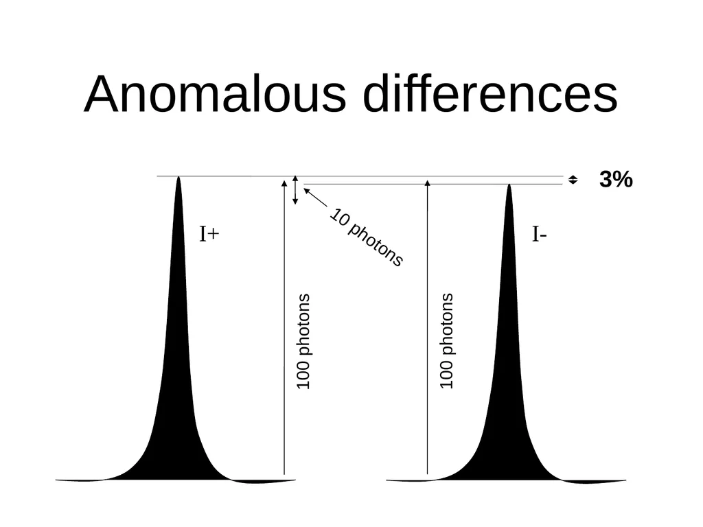
Anomalous differences I- I+ 100 photons<br>
20
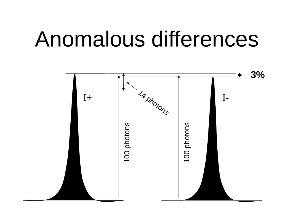
Anomalous differences I- I+<br>
21
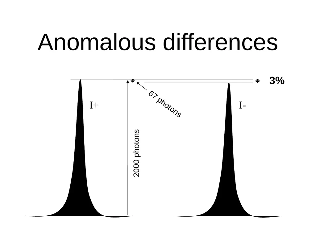
Anomalous differences 3% I- I+ 2000 photons<br>
22
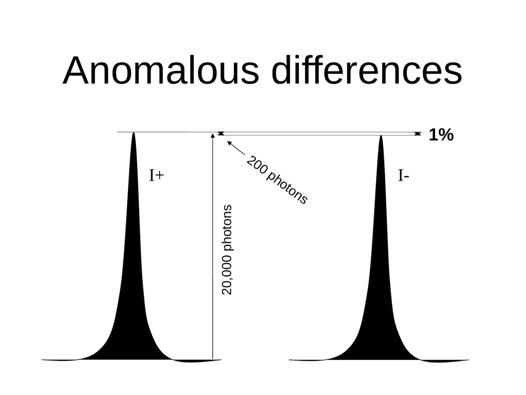
Anomalous differences 1% I- I+ 20,000 photons<br>
23
Can you count to 1,000,000 ? = 0.1% Theoretically: In reality: ISa ~ 33 Rmeas ≈ 0.1% ?<br>
24
systematic error<br>
25
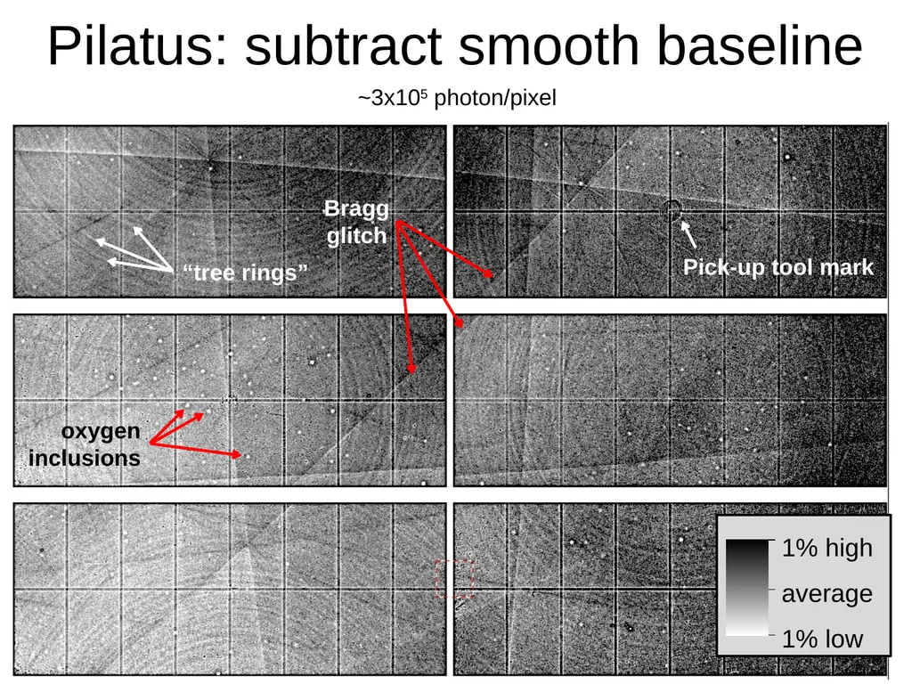
~3x10⁵ photon/pixel Pilatus: subtract smooth baseline<br>
26
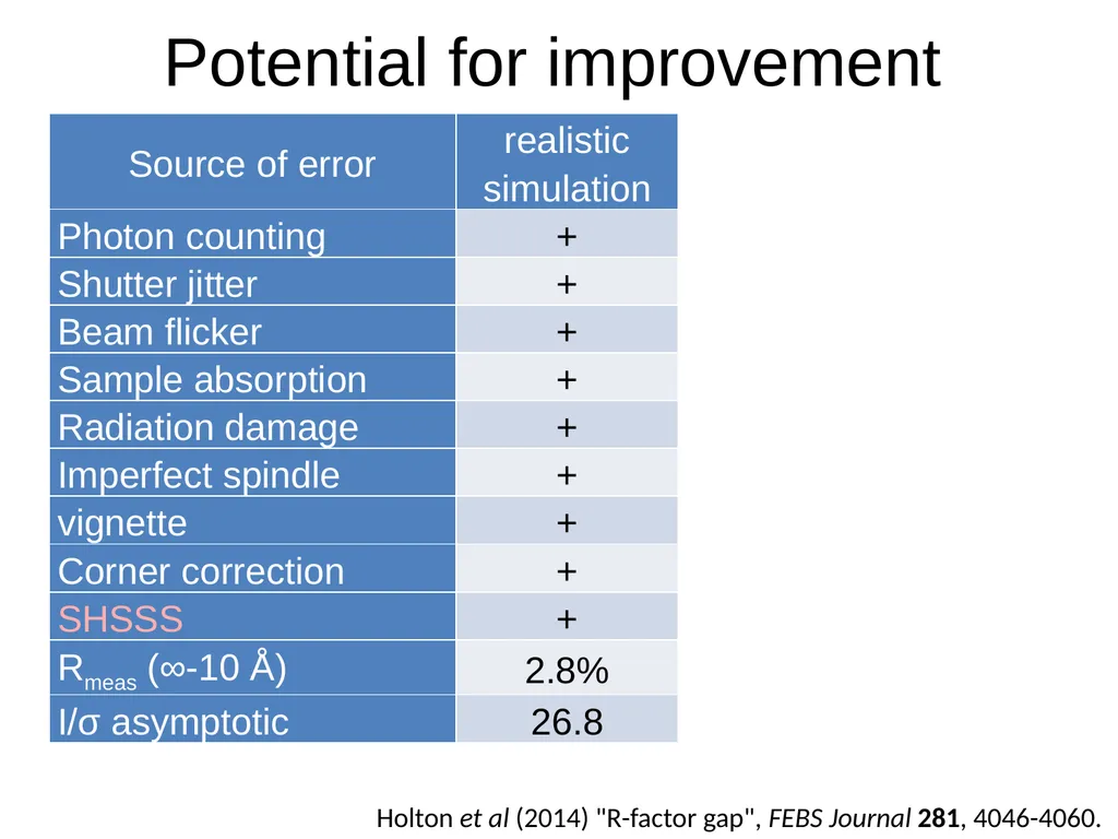
Potential for improvement Holton et al (2014) "R-factor gap", FEBS Journal 281, 4046-4060.<br>
27
Required signal-to-noise (I/σ) Solve-able proteins (%) Phasing from native elements<br>
28
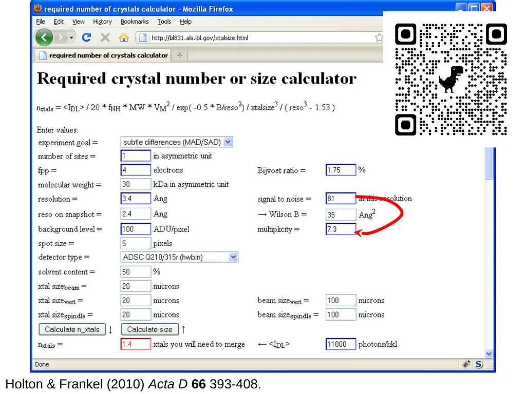
Holton & Frankel (2010) Acta D 66 393-408.<br>
29
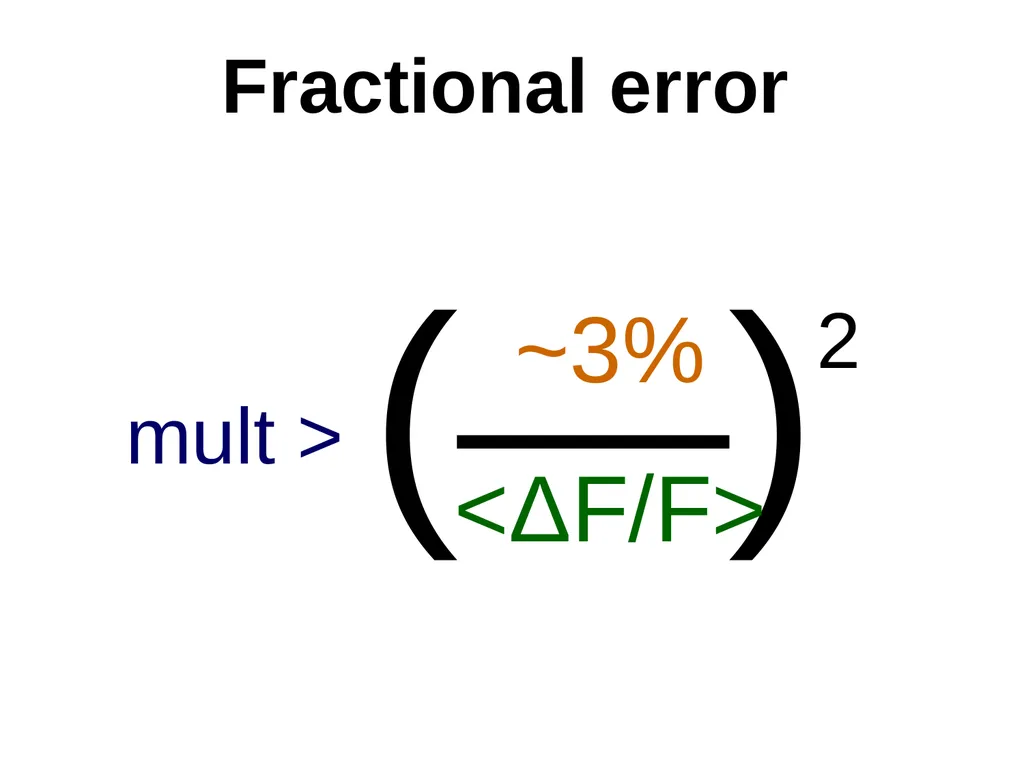
Fractional error mult > (—)2 ~3%
<ΔF/F><br>
<ΔF/F><br>
30
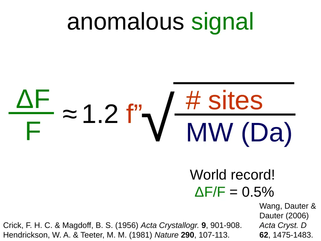
anomalous signal Crick, F. H. C. & Magdoff, B. S. (1956) Acta Crystallogr. 9, 901-908.
Hendrickson, W. A. & Teeter, M. M. (1981) Nature 290, 107-113. # sites
MW (Da) ≈ 1.2 f” World record!
ΔF/F = 0.5% Wang, Dauter & Dauter (2006) Acta Cryst. D 62, 1475-1483.<br>
Hendrickson, W. A. & Teeter, M. M. (1981) Nature 290, 107-113. # sites
MW (Da) ≈ 1.2 f” World record!
ΔF/F = 0.5% Wang, Dauter & Dauter (2006) Acta Cryst. D 62, 1475-1483.<br>
31
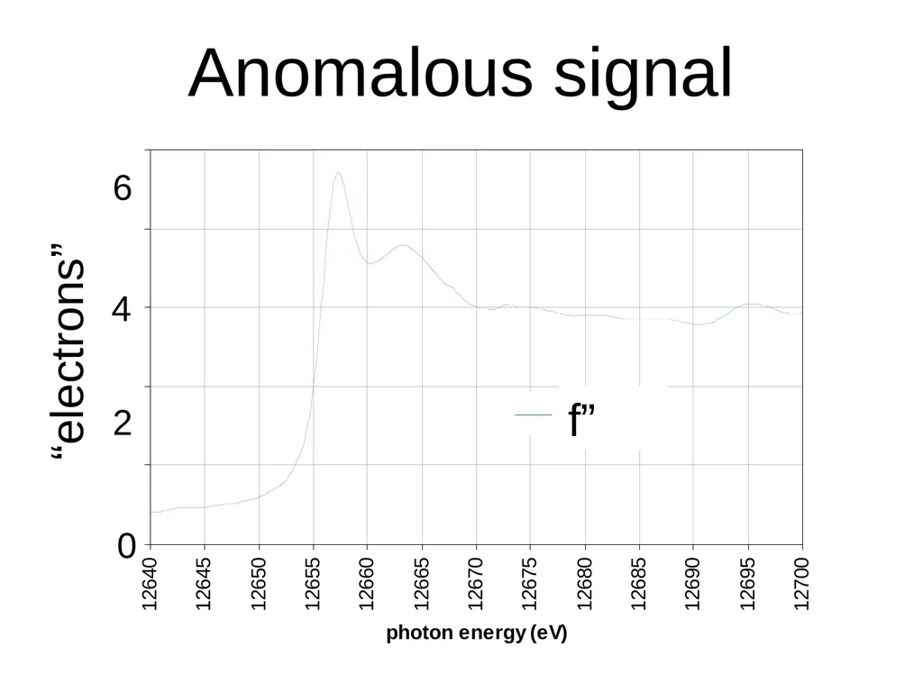
Anomalous signal 1 f” 4 6 0 2 “electrons”<br>
32
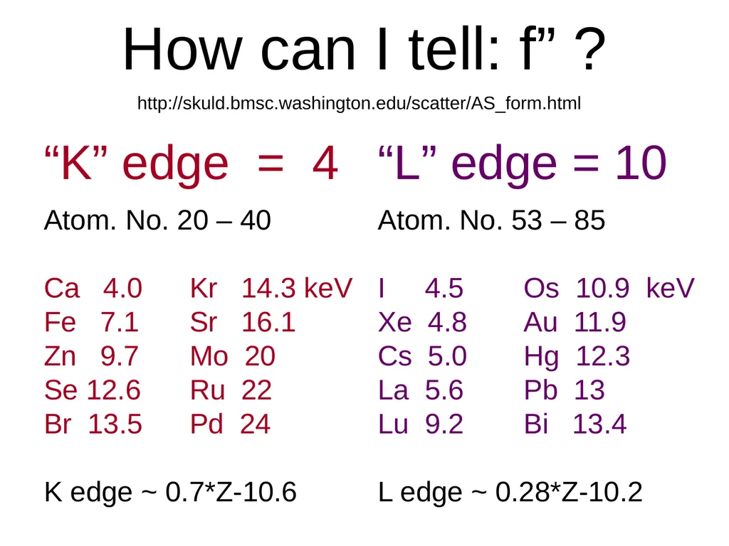
How can I tell: f” ? “K” edge = 4
Atom. No. 20 – 40
Ca 4.0 Kr 14.3 keV
Fe 7.1 Sr 16.1
Zn 9.7 Mo 20
Se 12.6 Ru 22
Br 13.5 Pd 24
K edge ~ 0.7*Z-10.6 “L” edge = 10
Atom. No. 53 – 85
I 4.5 Os 10.9 keV
Xe 4.8 Au 11.9
Cs 5.0 Hg 12.3
La 5.6 Pb 13
Lu 9.2 Bi 13.4
L edge ~ 0.28*Z-10.2 http://skuld.bmsc.washington.edu/scatter/AS_form.html<br>
Atom. No. 20 – 40
Ca 4.0 Kr 14.3 keV
Fe 7.1 Sr 16.1
Zn 9.7 Mo 20
Se 12.6 Ru 22
Br 13.5 Pd 24
K edge ~ 0.7*Z-10.6 “L” edge = 10
Atom. No. 53 – 85
I 4.5 Os 10.9 keV
Xe 4.8 Au 11.9
Cs 5.0 Hg 12.3
La 5.6 Pb 13
Lu 9.2 Bi 13.4
L edge ~ 0.28*Z-10.2 http://skuld.bmsc.washington.edu/scatter/AS_form.html<br>
33
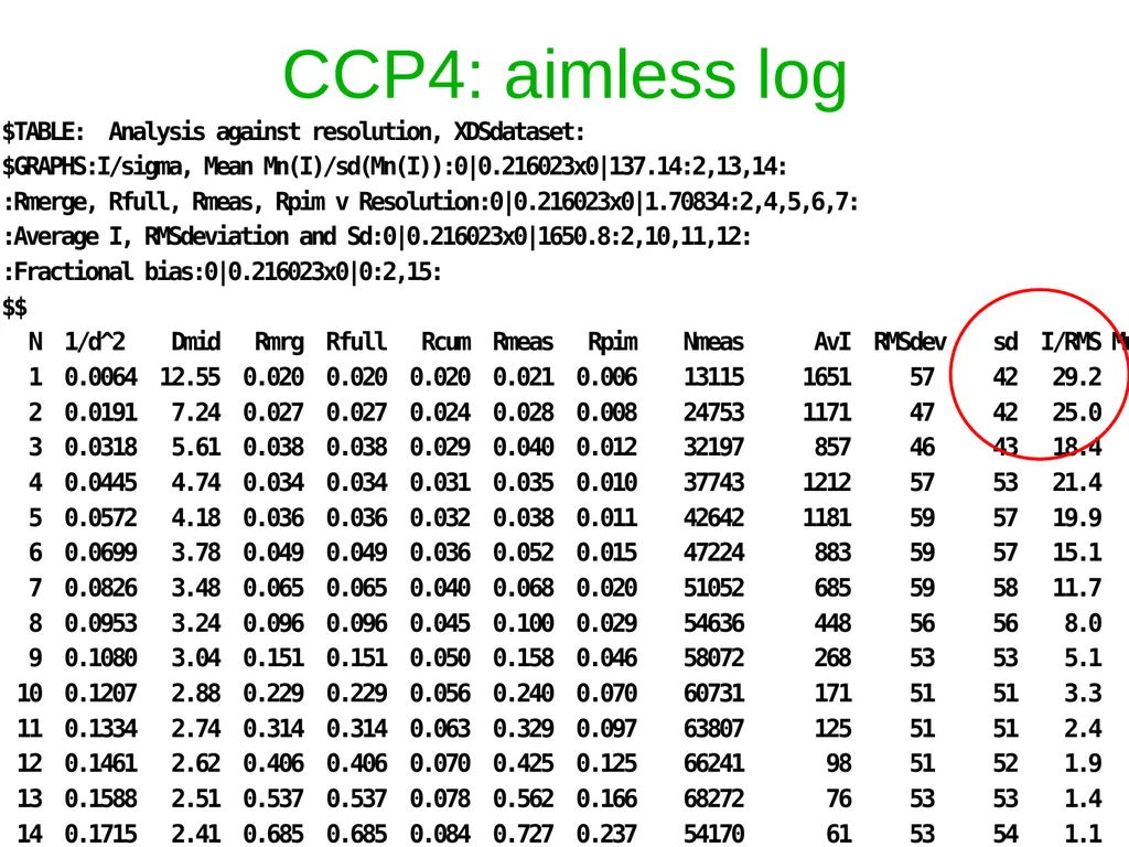
CCP4: aimless log $TABLE: Analysis against resolution, XDSdataset:
$GRAPHS:I/sigma, Mean Mn(I)/sd(Mn(I)):0|0.216023x0|137.14:2,13,14:
:Rmerge, Rfull, Rmeas, Rpim v Resolution:0|0.216023x0|1.70834:2,4,5,6,7:
:Average I, RMSdeviation and Sd:0|0.216023x0|1650.8:2,10,11,12:
:Fractional bias:0|0.216023x0|0:2,15:
$$
N 1/d^2 Dmid Rmrg Rfull Rcum Rmeas Rpim Nmeas AvI RMSdev sd I/RMS Mn(I/sd) FrcBias $$ $$
1 0.0064 12.55 0.020 0.020 0.020 0.021 0.006 13115 1651 57 42 29.2 137.1 -
2 0.0191 7.24 0.027 0.027 0.024 0.028 0.008 24753 1171 47 42 25.0 105.2 -
3 0.0318 5.61 0.038 0.038 0.029 0.040 0.012 32197 857 46 43 18.4 79.6 -
4 0.0445 4.74 0.034 0.034 0.031 0.035 0.010 37743 1212 57 53 21.4 91.2 -
5 0.0572 4.18 0.036 0.036 0.032 0.038 0.011 42642 1181 59 57 19.9 83.8 -
6 0.0699 3.78 0.049 0.049 0.036 0.052 0.015 47224 883 59 57 15.1 65.1 -
7 0.0826 3.48 0.065 0.065 0.040 0.068 0.020 51052 685 59 58 11.7 50.9 -
8 0.0953 3.24 0.096 0.096 0.045 0.100 0.029 54636 448 56 56 8.0 35.0 -
9 0.1080 3.04 0.151 0.151 0.050 0.158 0.046 58072 268 53 53 5.1 22.7 -
10 0.1207 2.88 0.229 0.229 0.056 0.240 0.070 60731 171 51 51 3.3 15.4 -
11 0.1334 2.74 0.314 0.314 0.063 0.329 0.097 63807 125 51 51 2.4 11.3 -
12 0.1461 2.62 0.406 0.406 0.070 0.425 0.125 66241 98 51 52 1.9 8.7 -
13 0.1588 2.51 0.537 0.537 0.078 0.562 0.166 68272 76 53 53 1.4 6.5 -
14 0.1715 2.41 0.685 0.685 0.084 0.727 0.237 54170 61 53 54 1.1 4.4 -
15 0.1843 2.33 0.886 0.886 0.088 0.950 0.333 39781 48 55 56 0.9 3.1 -
16 0.1970 2.25 1.249 1.249 0.092 1.355 0.508 29754 35 57 59 0.6 2.1 -<br>
$GRAPHS:I/sigma, Mean Mn(I)/sd(Mn(I)):0|0.216023x0|137.14:2,13,14:
:Rmerge, Rfull, Rmeas, Rpim v Resolution:0|0.216023x0|1.70834:2,4,5,6,7:
:Average I, RMSdeviation and Sd:0|0.216023x0|1650.8:2,10,11,12:
:Fractional bias:0|0.216023x0|0:2,15:
$$
N 1/d^2 Dmid Rmrg Rfull Rcum Rmeas Rpim Nmeas AvI RMSdev sd I/RMS Mn(I/sd) FrcBias $$ $$
1 0.0064 12.55 0.020 0.020 0.020 0.021 0.006 13115 1651 57 42 29.2 137.1 -
2 0.0191 7.24 0.027 0.027 0.024 0.028 0.008 24753 1171 47 42 25.0 105.2 -
3 0.0318 5.61 0.038 0.038 0.029 0.040 0.012 32197 857 46 43 18.4 79.6 -
4 0.0445 4.74 0.034 0.034 0.031 0.035 0.010 37743 1212 57 53 21.4 91.2 -
5 0.0572 4.18 0.036 0.036 0.032 0.038 0.011 42642 1181 59 57 19.9 83.8 -
6 0.0699 3.78 0.049 0.049 0.036 0.052 0.015 47224 883 59 57 15.1 65.1 -
7 0.0826 3.48 0.065 0.065 0.040 0.068 0.020 51052 685 59 58 11.7 50.9 -
8 0.0953 3.24 0.096 0.096 0.045 0.100 0.029 54636 448 56 56 8.0 35.0 -
9 0.1080 3.04 0.151 0.151 0.050 0.158 0.046 58072 268 53 53 5.1 22.7 -
10 0.1207 2.88 0.229 0.229 0.056 0.240 0.070 60731 171 51 51 3.3 15.4 -
11 0.1334 2.74 0.314 0.314 0.063 0.329 0.097 63807 125 51 51 2.4 11.3 -
12 0.1461 2.62 0.406 0.406 0.070 0.425 0.125 66241 98 51 52 1.9 8.7 -
13 0.1588 2.51 0.537 0.537 0.078 0.562 0.166 68272 76 53 53 1.4 6.5 -
14 0.1715 2.41 0.685 0.685 0.084 0.727 0.237 54170 61 53 54 1.1 4.4 -
15 0.1843 2.33 0.886 0.886 0.088 0.950 0.333 39781 48 55 56 0.9 3.1 -
16 0.1970 2.25 1.249 1.249 0.092 1.355 0.508 29754 35 57 59 0.6 2.1 -<br>
34
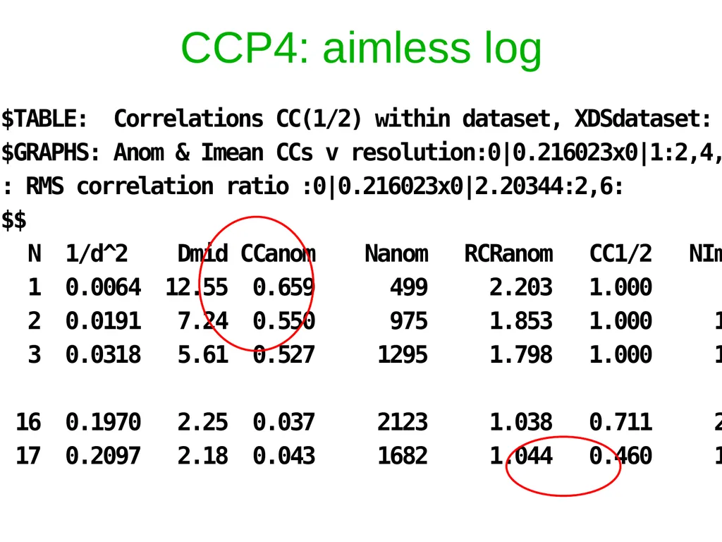
CCP4: aimless log $TABLE: Correlations CC(1/2) within dataset, XDSdataset:
$GRAPHS: Anom & Imean CCs v resolution:0|0.216023x0|1:2,4,7:
: RMS correlation ratio :0|0.216023x0|2.20344:2,6:
$$
N 1/d^2 Dmid CCanom Nanom RCRanom CC1/2 NImean $$ $$
1 0.0064 12.55 0.659 499 2.203 1.000 669
2 0.0191 7.24 0.550 975 1.853 1.000 1155
3 0.0318 5.61 0.527 1295 1.798 1.000 1479
16 0.1970 2.25 0.037 2123 1.038 0.711 2275
17 0.2097 2.18 0.043 1682 1.044 0.460 1877<br>
$GRAPHS: Anom & Imean CCs v resolution:0|0.216023x0|1:2,4,7:
: RMS correlation ratio :0|0.216023x0|2.20344:2,6:
$$
N 1/d^2 Dmid CCanom Nanom RCRanom CC1/2 NImean $$ $$
1 0.0064 12.55 0.659 499 2.203 1.000 669
2 0.0191 7.24 0.550 975 1.853 1.000 1155
3 0.0318 5.61 0.527 1295 1.798 1.000 1479
16 0.1970 2.25 0.037 2123 1.038 0.711 2275
17 0.2097 2.18 0.043 1682 1.044 0.460 1877<br>
35
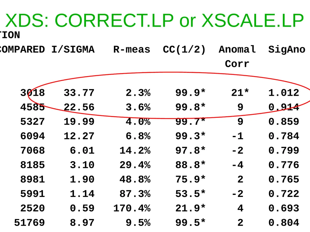
XDS: CORRECT.LP or XSCALE.LP SUBSET OF INTENSITY DATA WITH SIGNAL/NOISE >= -3.0 AS FUNCTION OF RESOLUTION
RESOLUTION NUMBER OF REFLECTIONS COMPLETENESS R-FACTOR R-FACTOR COMPARED I/SIGMA R-meas CC(1/2) Anomal SigAno Nano
LIMIT OBSERVED UNIQUE POSSIBLE OF DATA observed expected Corr
6.39 4103 2517 3135 80.3% 1.7% 1.8% 3018 33.77 2.3% 99.9* 21* 1.012 533
4.54 7339 4970 5544 89.6% 2.6% 2.6% 4585 22.56 3.6% 99.8* 9 0.914 796
3.72 9442 6724 7186 93.6% 2.8% 2.9% 5327 19.99 4.0% 99.7* 9 0.859 877
3.22 11077 7997 8486 94.2% 4.8% 4.9% 6094 12.27 6.8% 99.3* -1 0.784 913
2.88 12408 8851 9595 92.2% 10.0% 10.1% 7068 6.01 14.2% 97.8* -2 0.799 1012
2.63 13673 9561 10662 89.7% 20.8% 20.8% 8185 3.10 29.4% 88.8* -4 0.776 1274
2.44 14360 9852 11510 85.6% 34.5% 34.7% 8981 1.90 48.8% 75.9* 2 0.765 1525
2.28 9501 6495 12416 52.3% 61.8% 59.6% 5991 1.14 87.3% 53.5* -2 0.722 1031
2.15 4567 3307 13210 25.0% 120.5% 120.3% 2520 0.59 170.4% 21.9* 4 0.693 408
total 86470 60274 81744 73.7% 6.7% 6.7% 51769 8.97 9.5% 99.5* 2 0.804 8369<br>
RESOLUTION NUMBER OF REFLECTIONS COMPLETENESS R-FACTOR R-FACTOR COMPARED I/SIGMA R-meas CC(1/2) Anomal SigAno Nano
LIMIT OBSERVED UNIQUE POSSIBLE OF DATA observed expected Corr
6.39 4103 2517 3135 80.3% 1.7% 1.8% 3018 33.77 2.3% 99.9* 21* 1.012 533
4.54 7339 4970 5544 89.6% 2.6% 2.6% 4585 22.56 3.6% 99.8* 9 0.914 796
3.72 9442 6724 7186 93.6% 2.8% 2.9% 5327 19.99 4.0% 99.7* 9 0.859 877
3.22 11077 7997 8486 94.2% 4.8% 4.9% 6094 12.27 6.8% 99.3* -1 0.784 913
2.88 12408 8851 9595 92.2% 10.0% 10.1% 7068 6.01 14.2% 97.8* -2 0.799 1012
2.63 13673 9561 10662 89.7% 20.8% 20.8% 8185 3.10 29.4% 88.8* -4 0.776 1274
2.44 14360 9852 11510 85.6% 34.5% 34.7% 8981 1.90 48.8% 75.9* 2 0.765 1525
2.28 9501 6495 12416 52.3% 61.8% 59.6% 5991 1.14 87.3% 53.5* -2 0.722 1031
2.15 4567 3307 13210 25.0% 120.5% 120.3% 2520 0.59 170.4% 21.9* 4 0.693 408
total 86470 60274 81744 73.7% 6.7% 6.7% 51769 8.97 9.5% 99.5* 2 0.804 8369<br>
36
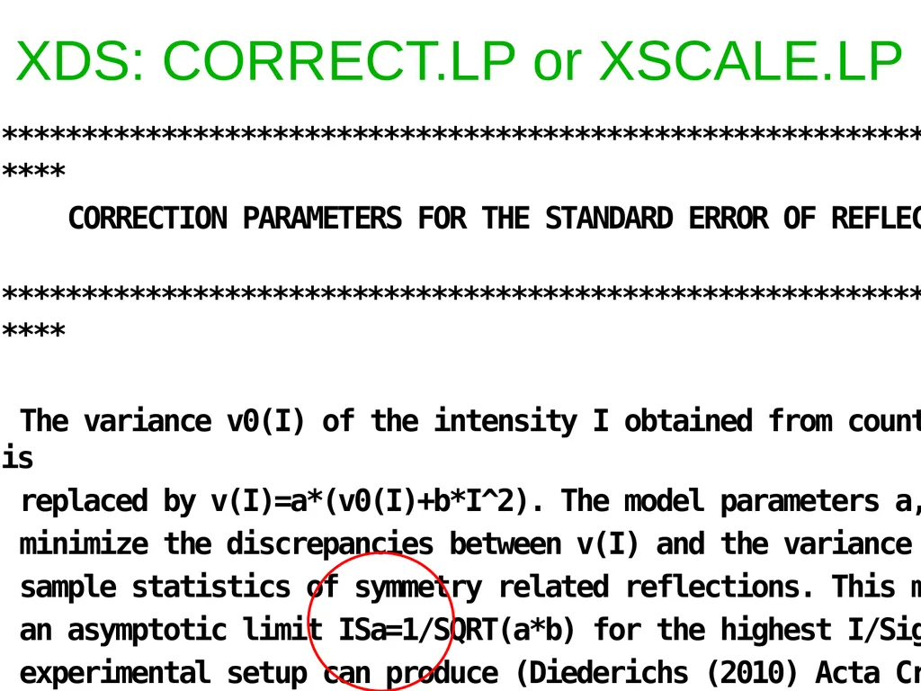
XDS: CORRECT.LP or XSCALE.LP ******************************************************************************
CORRECTION PARAMETERS FOR THE STANDARD ERROR OF REFLECTION INTENSITIES
******************************************************************************
The variance v0(I) of the intensity I obtained from counting statistics is
replaced by v(I)=a*(v0(I)+b*I^2). The model parameters a, b are chosen to
minimize the discrepancies between v(I) and the variance estimated from
sample statistics of symmetry related reflections. This model implicates
an asymptotic limit ISa=1/SQRT(a*b) for the highest I/Sigma(I) that the
experimental setup can produce (Diederichs (2010) Acta Cryst D66, 733-740).
a b ISa
3.806E+00 1.080E-04 49.32<br>
CORRECTION PARAMETERS FOR THE STANDARD ERROR OF REFLECTION INTENSITIES
******************************************************************************
The variance v0(I) of the intensity I obtained from counting statistics is
replaced by v(I)=a*(v0(I)+b*I^2). The model parameters a, b are chosen to
minimize the discrepancies between v(I) and the variance estimated from
sample statistics of symmetry related reflections. This model implicates
an asymptotic limit ISa=1/SQRT(a*b) for the highest I/Sigma(I) that the
experimental setup can produce (Diederichs (2010) Acta Cryst D66, 733-740).
a b ISa
3.806E+00 1.080E-04 49.32<br>
37
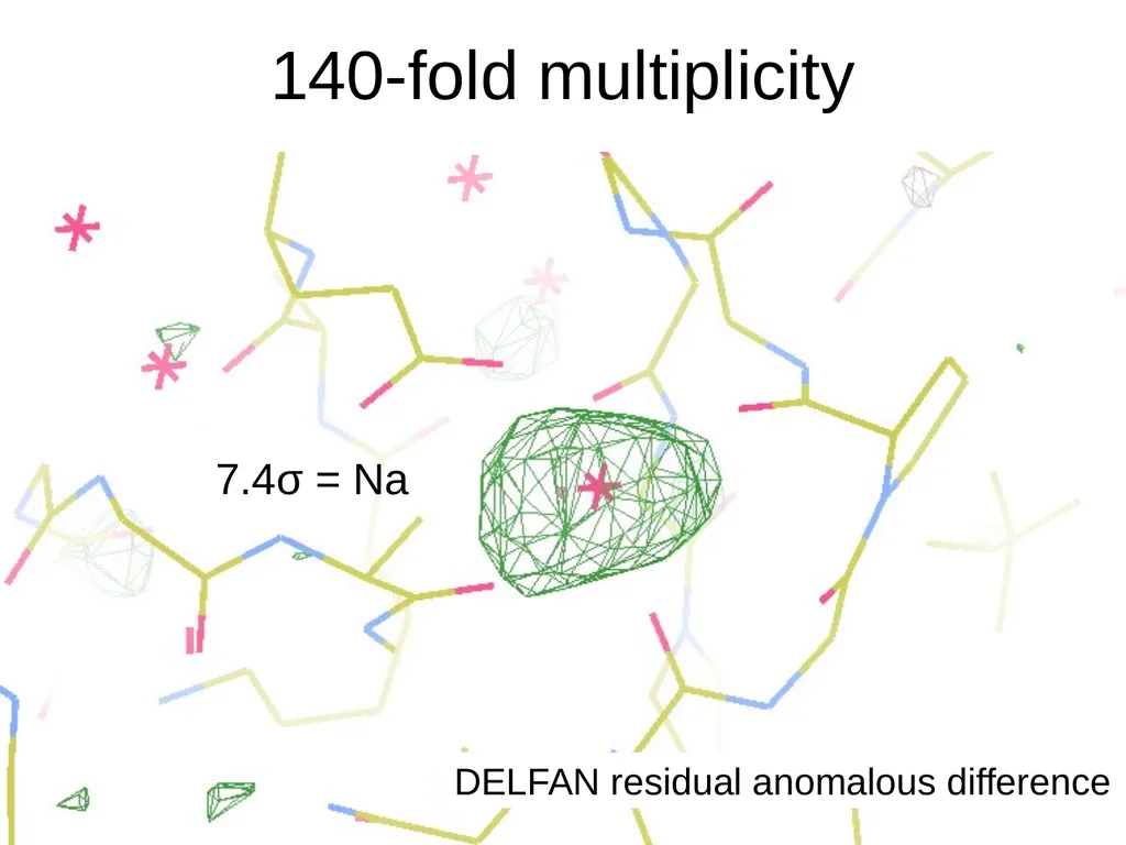
140-fold multiplicity 7.4σ = Na DELFAN residual anomalous difference<br>
38
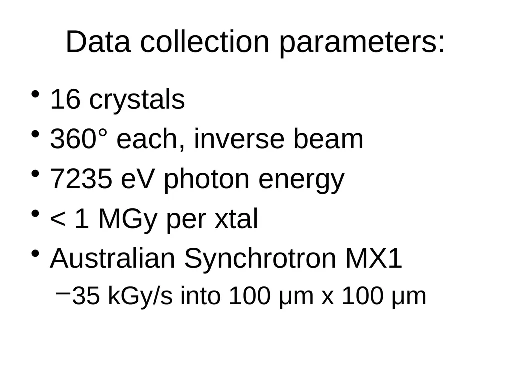
Data collection parameters: 16 crystals
360° each, inverse beam
7235 eV photon energy
< 1 MGy per xtal
Australian Synchrotron MX1
35 kGy/s into 100 μm x 100 μm<br>
360° each, inverse beam
7235 eV photon energy
< 1 MGy per xtal
Australian Synchrotron MX1
35 kGy/s into 100 μm x 100 μm<br>
39
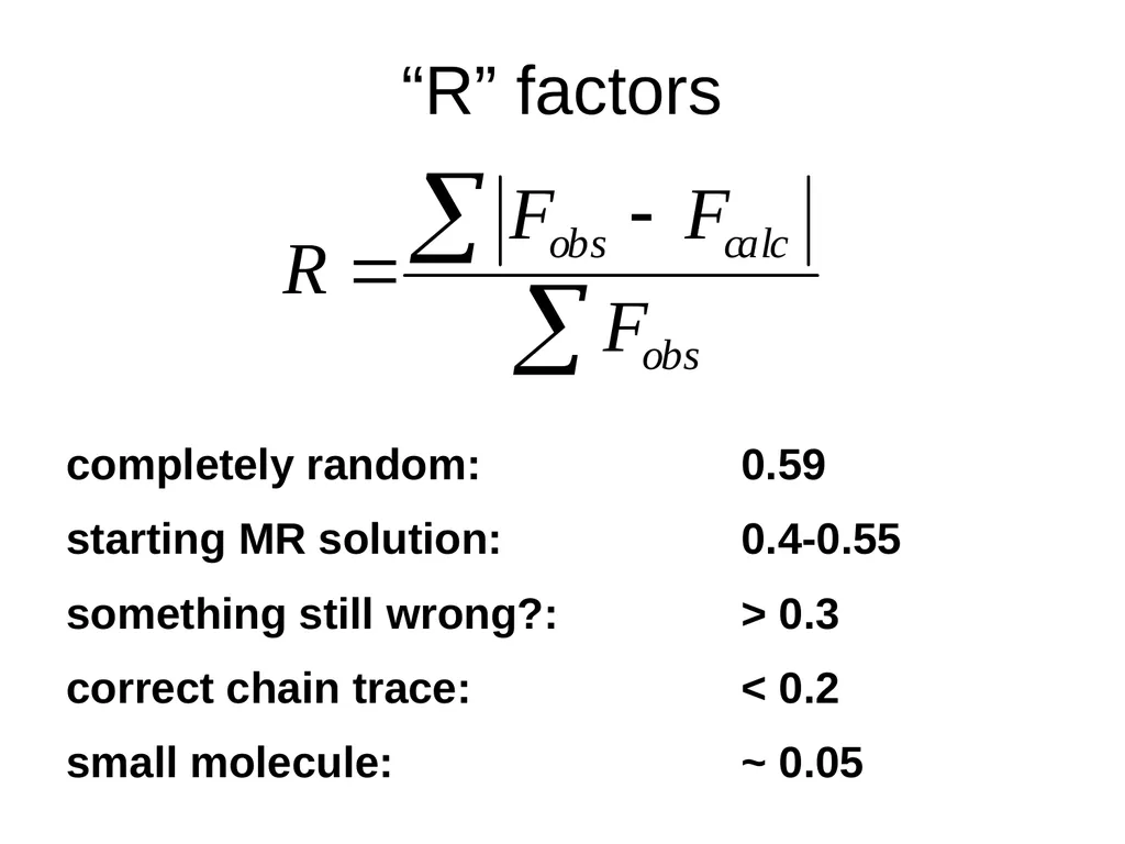
“R” factors R = % error<br>
40
“R” factors completely random: 0.59
starting MR solution: 0.4-0.55
something still wrong?: > 0.3
correct chain trace: < 0.2
small molecule: ~ 0.05<br>
starting MR solution: 0.4-0.55
something still wrong?: > 0.3
correct chain trace: < 0.2
small molecule: ~ 0.05<br>
41
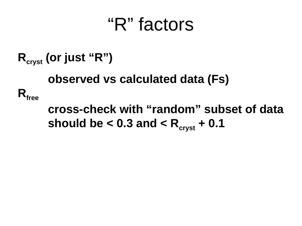
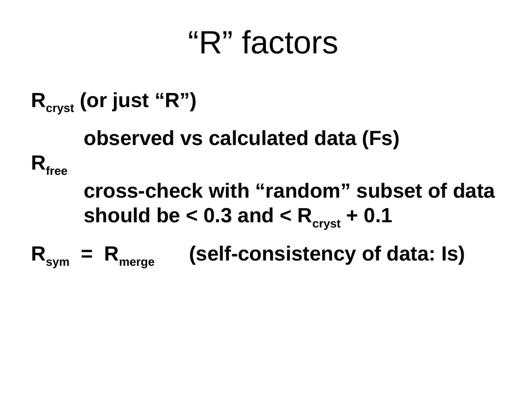
“R” factors Rcryst (or just “R”)
observed vs calculated data (Fs)
Rfree
cross-check with “random” subset of data
should be < 0.3 and < Rcryst + 0.1<br>
observed vs calculated data (Fs)
Rfree
cross-check with “random” subset of data
should be < 0.3 and < Rcryst + 0.1<br>
42
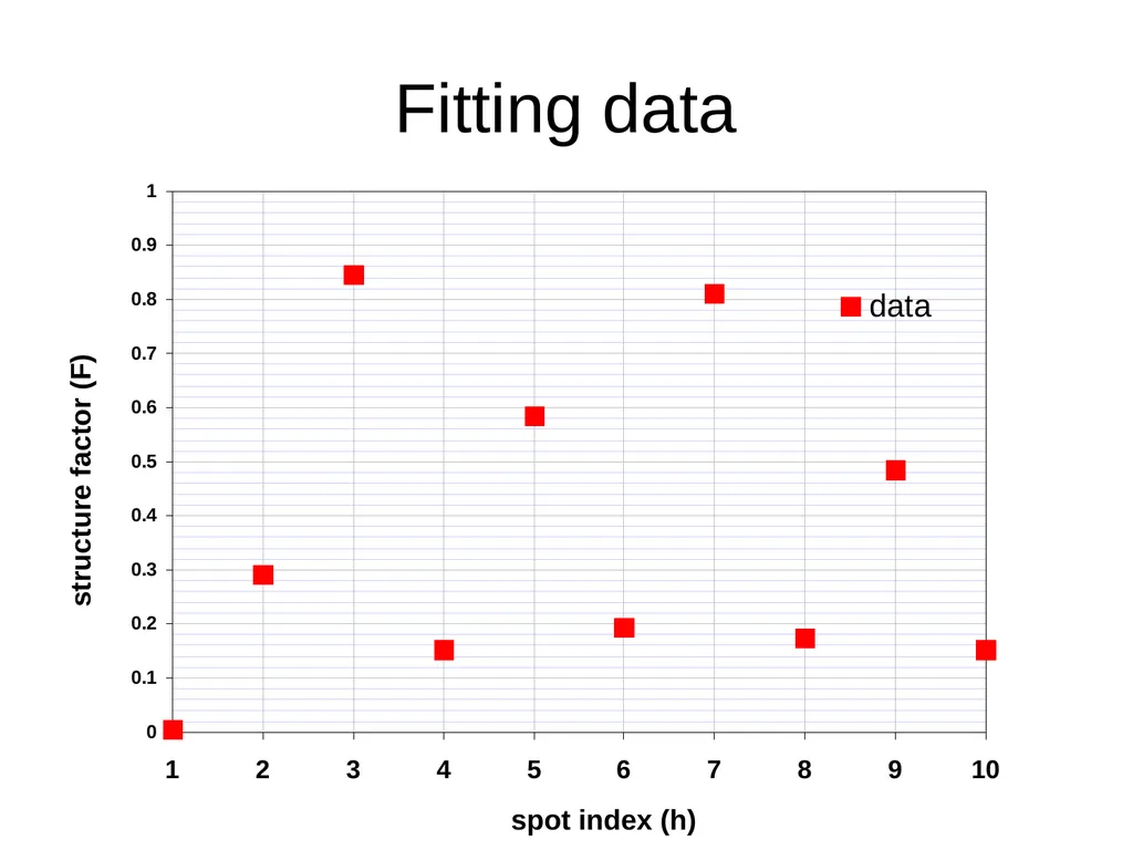
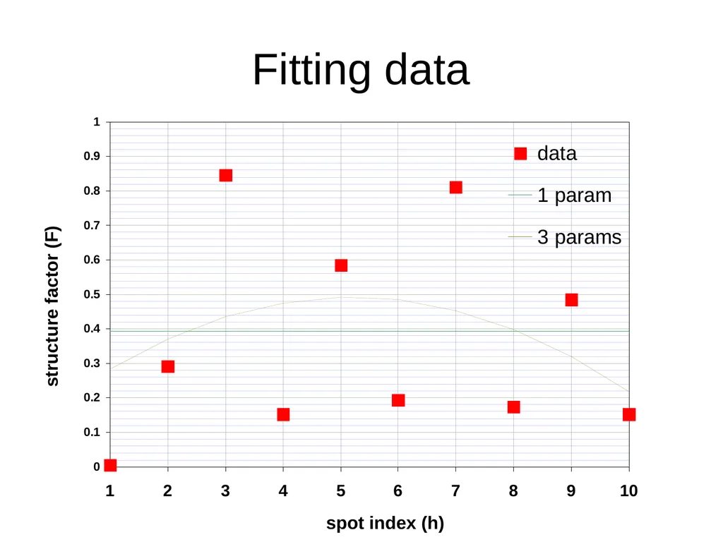
structure factor (F) spot index (h) Fitting data<br>
43
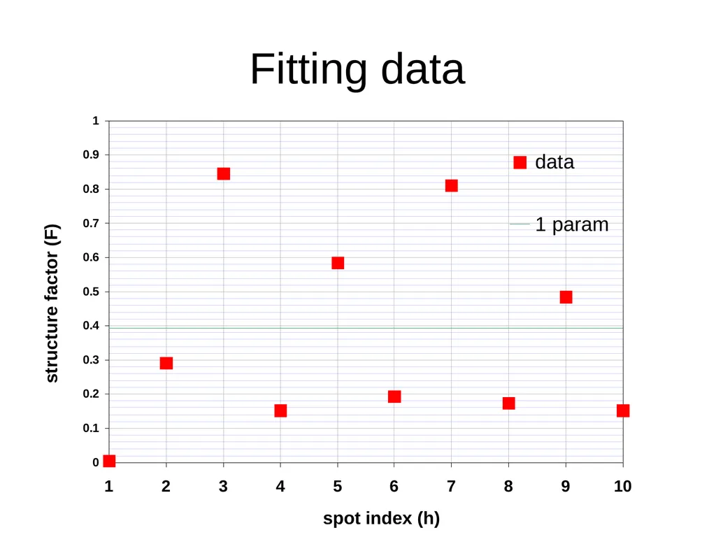
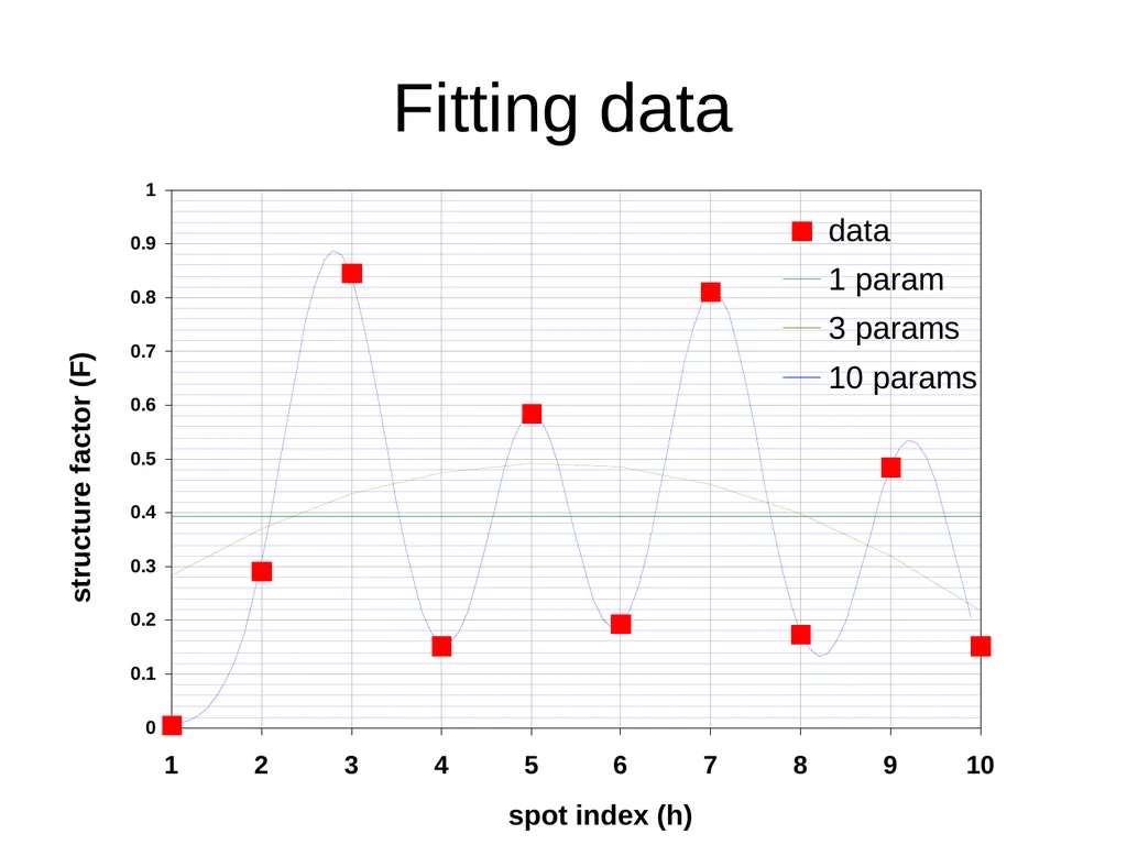
structure factor (F) spot index (h) Fitting data<br>
44
structure factor (F) spot index (h) Fitting data<br>
45
structure factor (F) spot index (h) Fitting data<br>
46
“R” factors Rcryst (or just “R”)
observed vs calculated data (Fs)
Rfree
cross-check with “random” subset of data
should be < 0.3 and < Rcryst + 0.1
Rsym = Rmerge (self-consistency of data: Is)<br>
observed vs calculated data (Fs)
Rfree
cross-check with “random” subset of data
should be < 0.3 and < Rcryst + 0.1
Rsym = Rmerge (self-consistency of data: Is)<br>
47
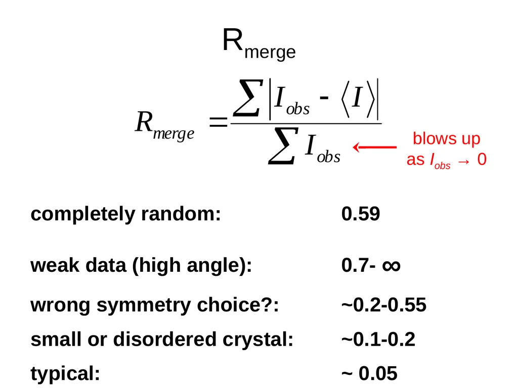
Rmerge completely random: 0.59
weak data (high angle): 0.7- ∞
wrong symmetry choice?: ~0.2-0.55
small or disordered crystal: ~0.1-0.2
typical: ~ 0.05<br>
weak data (high angle): 0.7- ∞
wrong symmetry choice?: ~0.2-0.55
small or disordered crystal: ~0.1-0.2
typical: ~ 0.05<br>
48
“R” factors Rcryst (or just “R”)
observed vs calculated data (Fs)
Rfree
cross-check with “random” subset of data
should be < 0.3 and < Rcryst + 0.1
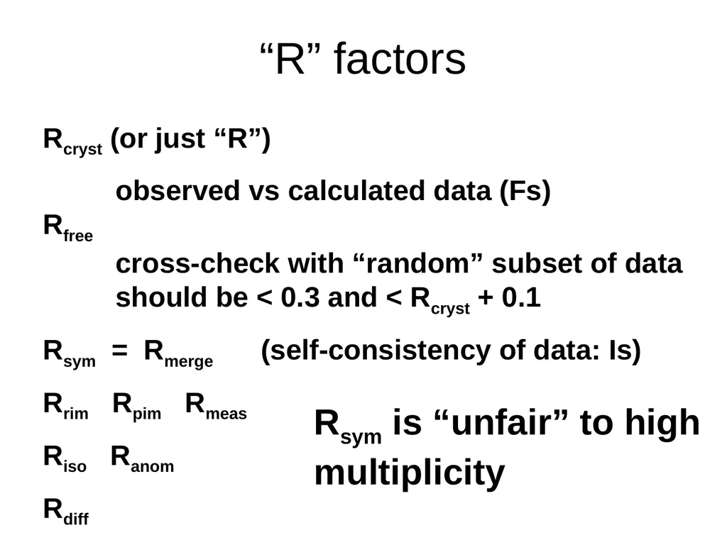
Rsym = Rmerge (self-consistency of data: Is)
Rrim Rpim Rmeas
Riso Ranom
Rdiff Rsym is “unfair” to high multiplicity<br>
observed vs calculated data (Fs)
Rfree
cross-check with “random” subset of data
should be < 0.3 and < Rcryst + 0.1
Rsym = Rmerge (self-consistency of data: Is)
Rrim Rpim Rmeas
Riso Ranom
Rdiff Rsym is “unfair” to high multiplicity<br>