Scaling Up Machine Learning Parallel and

aaron

Published 2026-08-27 . 0 views

↓ Download

Scaling Up Machine Learning Parallel and

Scaling Up Machine Learning Parallel and - slide 1 of 114

Scaling Up Machine Learning Parallel and - slide 2 of 114

Scaling Up Machine Learning Parallel and - slide 3 of 114

Scaling Up Machine Learning Parallel and - slide 4 of 114

Scaling Up Machine Learning Parallel and - slide 5 of 114

Scaling Up Machine Learning Parallel and - slide 6 of 114

Scaling Up Machine Learning Parallel and - slide 7 of 114

Scaling Up Machine Learning Parallel and - slide 8 of 114

Scaling Up Machine Learning Parallel and - slide 9 of 114

Scaling Up Machine Learning Parallel and - slide 10 of 114

Scaling Up Machine Learning Parallel and - slide 11 of 114

Scaling Up Machine Learning Parallel and - slide 12 of 114

Scaling Up Machine Learning Parallel and - slide 13 of 114

Scaling Up Machine Learning Parallel and - slide 14 of 114

Scaling Up Machine Learning Parallel and - slide 15 of 114

Scaling Up Machine Learning Parallel and - slide 16 of 114

Scaling Up Machine Learning Parallel and - slide 17 of 114

Scaling Up Machine Learning Parallel and - slide 18 of 114

Scaling Up Machine Learning Parallel and - slide 19 of 114

Scaling Up Machine Learning Parallel and - slide 20 of 114

Scaling Up Machine Learning Parallel and - slide 21 of 114

Scaling Up Machine Learning Parallel and - slide 22 of 114

Scaling Up Machine Learning Parallel and - slide 23 of 114

Scaling Up Machine Learning Parallel and - slide 24 of 114

Scaling Up Machine Learning Parallel and - slide 25 of 114

Scaling Up Machine Learning Parallel and - slide 26 of 114

Scaling Up Machine Learning Parallel and - slide 27 of 114

Scaling Up Machine Learning Parallel and - slide 28 of 114

Scaling Up Machine Learning Parallel and - slide 29 of 114

Scaling Up Machine Learning Parallel and - slide 30 of 114

Scaling Up Machine Learning Parallel and - slide 31 of 114

Scaling Up Machine Learning Parallel and - slide 32 of 114

Scaling Up Machine Learning Parallel and - slide 33 of 114

Scaling Up Machine Learning Parallel and - slide 34 of 114

Scaling Up Machine Learning Parallel and - slide 35 of 114

Scaling Up Machine Learning Parallel and - slide 36 of 114

Scaling Up Machine Learning Parallel and - slide 37 of 114

Scaling Up Machine Learning Parallel and - slide 38 of 114

Scaling Up Machine Learning Parallel and - slide 39 of 114

Scaling Up Machine Learning Parallel and - slide 40 of 114

Scaling Up Machine Learning Parallel and - slide 41 of 114

Scaling Up Machine Learning Parallel and - slide 42 of 114

Scaling Up Machine Learning Parallel and - slide 43 of 114

Scaling Up Machine Learning Parallel and - slide 44 of 114

Scaling Up Machine Learning Parallel and - slide 45 of 114

Scaling Up Machine Learning Parallel and - slide 46 of 114

Scaling Up Machine Learning Parallel and - slide 47 of 114

Scaling Up Machine Learning Parallel and - slide 48 of 114

Scaling Up Machine Learning Parallel and - slide 49 of 114

Scaling Up Machine Learning Parallel and - slide 50 of 114

Scaling Up Machine Learning Parallel and - slide 51 of 114

Scaling Up Machine Learning Parallel and - slide 52 of 114

Scaling Up Machine Learning Parallel and - slide 53 of 114

Scaling Up Machine Learning Parallel and - slide 54 of 114

Scaling Up Machine Learning Parallel and - slide 55 of 114

Scaling Up Machine Learning Parallel and - slide 56 of 114

Scaling Up Machine Learning Parallel and - slide 57 of 114

Scaling Up Machine Learning Parallel and - slide 58 of 114

Scaling Up Machine Learning Parallel and - slide 59 of 114

Scaling Up Machine Learning Parallel and - slide 60 of 114

Scaling Up Machine Learning Parallel and - slide 61 of 114

Scaling Up Machine Learning Parallel and - slide 62 of 114

Scaling Up Machine Learning Parallel and - slide 63 of 114

Scaling Up Machine Learning Parallel and - slide 64 of 114

Scaling Up Machine Learning Parallel and - slide 65 of 114

Scaling Up Machine Learning Parallel and - slide 66 of 114

Scaling Up Machine Learning Parallel and - slide 67 of 114

Scaling Up Machine Learning Parallel and - slide 68 of 114

Scaling Up Machine Learning Parallel and - slide 69 of 114

Scaling Up Machine Learning Parallel and - slide 70 of 114

Scaling Up Machine Learning Parallel and - slide 71 of 114

Scaling Up Machine Learning Parallel and - slide 72 of 114

Scaling Up Machine Learning Parallel and - slide 73 of 114

Scaling Up Machine Learning Parallel and - slide 74 of 114

Scaling Up Machine Learning Parallel and - slide 75 of 114

Scaling Up Machine Learning Parallel and - slide 76 of 114

Scaling Up Machine Learning Parallel and - slide 77 of 114

Scaling Up Machine Learning Parallel and - slide 78 of 114

Scaling Up Machine Learning Parallel and - slide 79 of 114

Scaling Up Machine Learning Parallel and - slide 80 of 114

Scaling Up Machine Learning Parallel and - slide 81 of 114

Scaling Up Machine Learning Parallel and - slide 82 of 114

Scaling Up Machine Learning Parallel and - slide 83 of 114

Scaling Up Machine Learning Parallel and - slide 84 of 114

Scaling Up Machine Learning Parallel and - slide 85 of 114

Scaling Up Machine Learning Parallel and - slide 86 of 114

Scaling Up Machine Learning Parallel and - slide 87 of 114

Scaling Up Machine Learning Parallel and - slide 88 of 114

Scaling Up Machine Learning Parallel and - slide 89 of 114

Scaling Up Machine Learning Parallel and - slide 90 of 114

Scaling Up Machine Learning Parallel and - slide 91 of 114

Scaling Up Machine Learning Parallel and - slide 92 of 114

Scaling Up Machine Learning Parallel and - slide 93 of 114

Scaling Up Machine Learning Parallel and - slide 94 of 114

Scaling Up Machine Learning Parallel and - slide 95 of 114

Scaling Up Machine Learning Parallel and - slide 96 of 114

Scaling Up Machine Learning Parallel and - slide 97 of 114

Scaling Up Machine Learning Parallel and - slide 98 of 114

Scaling Up Machine Learning Parallel and - slide 99 of 114

Scaling Up Machine Learning Parallel and - slide 100 of 114

Scaling Up Machine Learning Parallel and - slide 101 of 114

Scaling Up Machine Learning Parallel and - slide 102 of 114

Scaling Up Machine Learning Parallel and - slide 103 of 114

Scaling Up Machine Learning Parallel and - slide 104 of 114

Scaling Up Machine Learning Parallel and - slide 105 of 114

Scaling Up Machine Learning Parallel and - slide 106 of 114

Scaling Up Machine Learning Parallel and - slide 107 of 114

Scaling Up Machine Learning Parallel and - slide 108 of 114

Scaling Up Machine Learning Parallel and - slide 109 of 114

Scaling Up Machine Learning Parallel and - slide 110 of 114

Scaling Up Machine Learning Parallel and - slide 111 of 114

Scaling Up Machine Learning Parallel and - slide 112 of 114

Scaling Up Machine Learning Parallel and - slide 113 of 114

Scaling Up Machine Learning Parallel and - slide 114 of 114

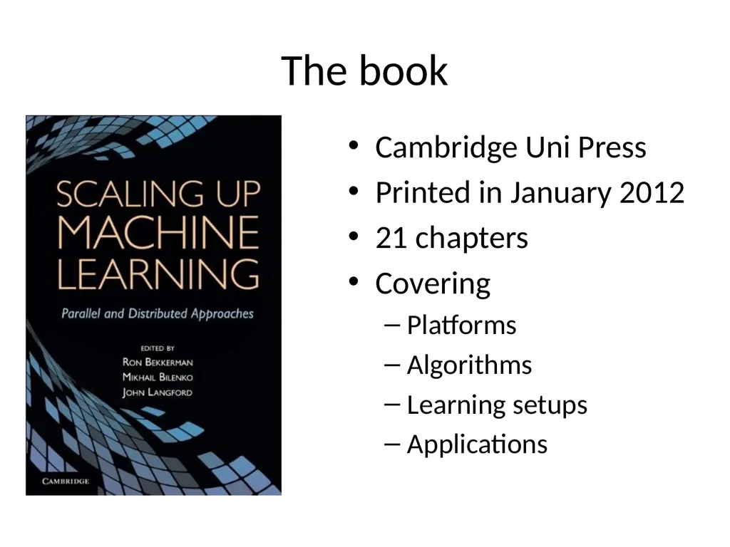
Description: Scaling Up Machine Learning Parallel and Distributed Approaches Ron Bekkerman, LinkedIn Misha Bilenko, MSR John Langford, Y!R http:hunch.netlargescalesurvey The book Cambridge Uni Press Printed in January 2012 21 chapters Covering

Download Presentation

"Scaling Up Machine Learning Parallel and" is the property of its rightful owner. Permission is granted to download and print the materials on this website for personal, non-commercial use only, and to display it on your personal computer provided you do not modify the materials and that you retain all copyright notices contained in the materials. By downloading content from our website, you accept the terms of this agreement.

Presentation Transcript

slide1. Scaling Up Machine Learning Parallel and Distributed Approaches Ron Bekkerman, LinkedIn
Misha Bilenko, MSR
John Langford, Y!R http://hunch.net/~large_scale_survey 
slide2. The book Cambridge Uni Press
Printed in January 2012
21 chapters
Covering
Platforms
Algorithms
Learning setups
Applications 
slide3. 10 2 Chapter contributors 3 4 5 6 7 8 9 11 12 13 14 15 16 17 18 19 20 21 
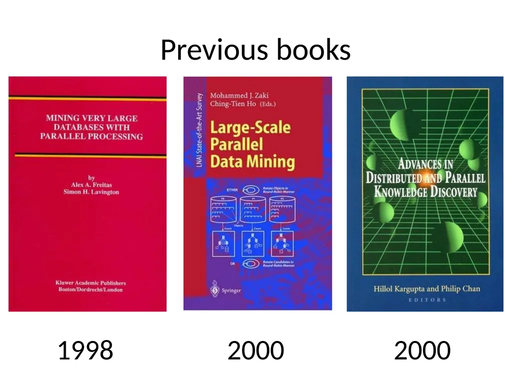
slide4. Previous books 1998 2000 2000 
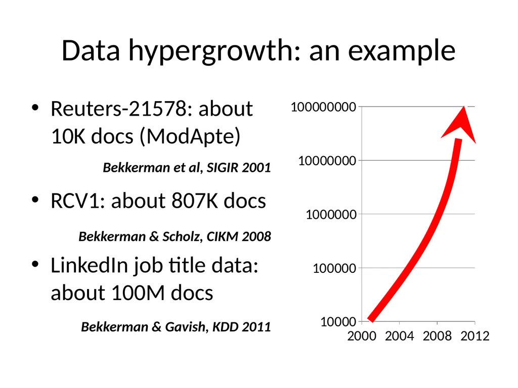
slide5. Data hypergrowth: an example Reuters-21578: about 10K docs (ModApte)

RCV1: about 807K docs

LinkedIn job title data: about 100M docs Bekkerman et al, SIGIR 2001 Bekkerman & Scholz, CIKM 2008 Bekkerman & Gavish, KDD 2011 
slide6. New age of big data The world has gone mobile
5 billion cellphones produce daily data
Social networks have gone online
Twitter produces 200M tweets a day
Crowdsourcing is the reality
Labeling of 100,000+ data instances is doable
Within a week  
slide7. Size matters One thousand data instances
One million data instances
One billion data instances
One trillion data instances

Those are not different numbers, those are different mindsets  
slide8. One thousand data instances Will process it manually within a day (a week?)
No need in an automatic approach
We shouldn’t publish main results on datasets of such size  
slide9. One million data instances Currently, the most active zone
Can be crowdsourced
Can be processed by a quadratic algorithm
Once parallelized
1M data collection cannot be too diverse
But can be too homogenous
Preprocessing / data probing is crucial 
slide10. Big datasets cannot be too sparse 1M data instances cannot belong to 1M classes
Simply because it’s not practical to have 1M classes 
Here’s a statistical experiment, in text domain:
1M documents
Each document is 100 words long
Randomly sampled from a unigram language model
No stopwords
245M pairs have word overlap of 10% or more
Real-world datasets are denser than random 
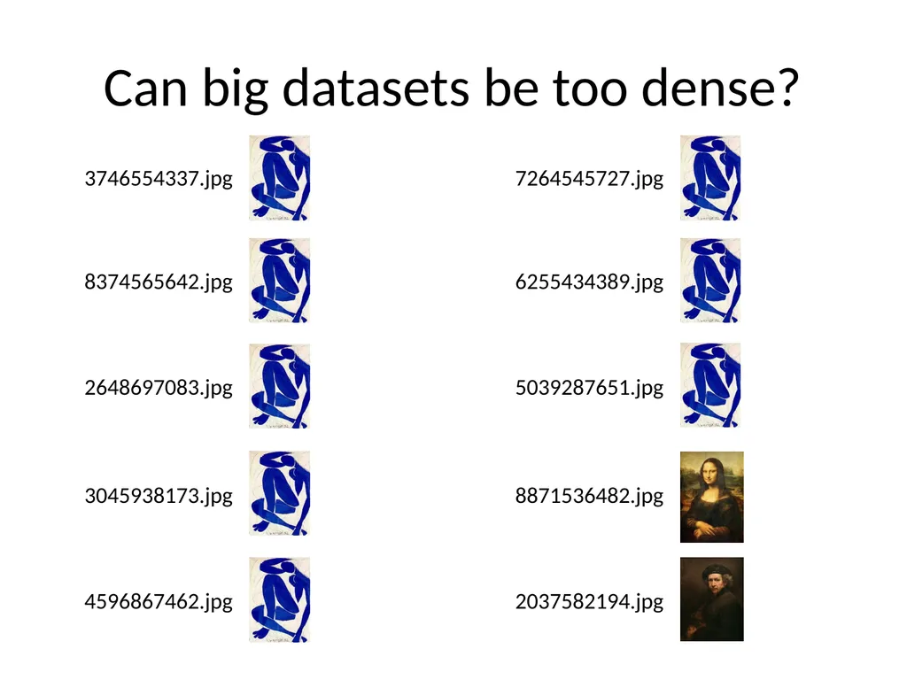
slide11. Can big datasets be too dense? 3746554337.jpg 8374565642.jpg 2648697083.jpg 7264545727.jpg 6255434389.jpg 5039287651.jpg 3045938173.jpg 4596867462.jpg 8871536482.jpg 2037582194.jpg 
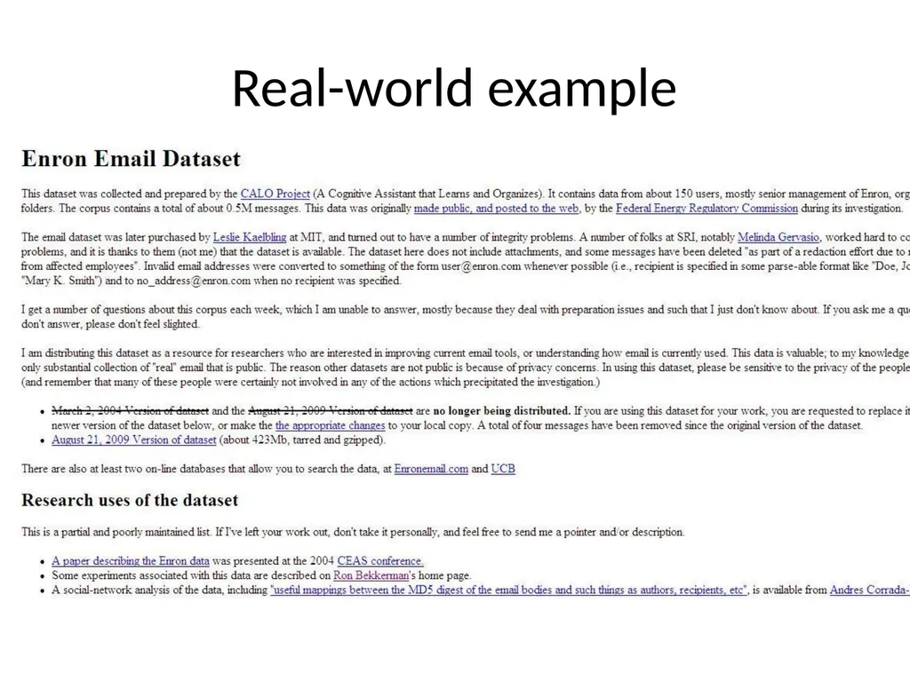
slide12. Real-world example 
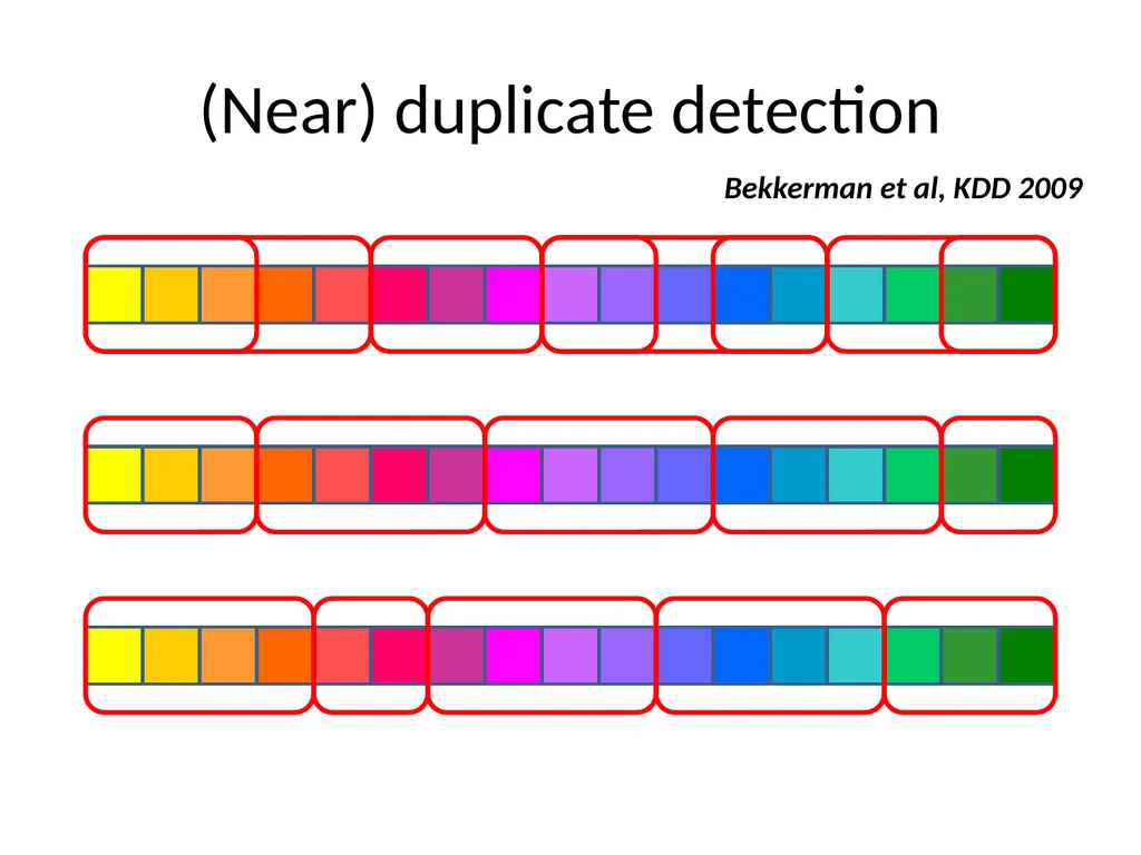
slide13. (Near) duplicate detection Bekkerman et al, KDD 2009 
slide14. One billion data instances Web-scale
Guaranteed to contain data in different formats
ASCII text, pictures, javascript code, PDF documents…
Guaranteed to contain (near) duplicates
Likely to be badly preprocessed 
Storage is an issue 
slide15. One trillion data instances Beyond the reach of the modern technology
Peer-to-peer paradigm is (arguably) the only way to process the data
Data privacy / inconsistency / skewness issues
Can’t be kept in one location
Is intrinsically hard to sample 
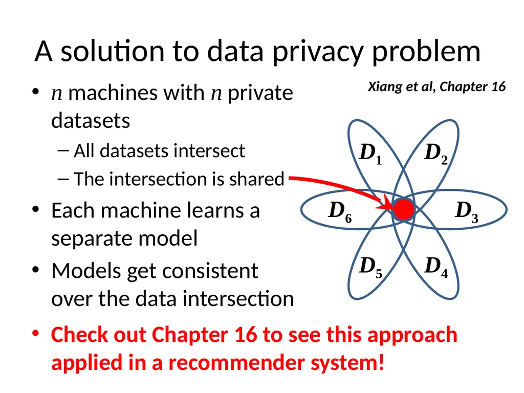
slide16. A solution to data privacy problem n machines with n private datasets
All datasets intersect
The intersection is shared
Each machine learns a separate model
Models get consistent over the data intersection Xiang et al, Chapter 16 D1 D2 D3 D4 D5 D6 Check out Chapter 16 to see this approach applied in a recommender system! 
slide17. So what model will we learn? Supervised model?
Unsupervised model?
Semi-supervised model?

Obviously, depending on the application 
But also on availability of labeled data
And its trustworthiness! 
slide18. Size of training data Say you have 1K labeled and 1M unlabeled examples
Labeled/unlabeled ratio: 0.1%
Is 1K enough to train a supervised model?
Now you have 1M labeled and 1B unlabeled examples
Labeled/unlabeled ratio: 0.1%
Is 1M enough to train a supervised model? 
slide19. Skewness of training data Usually, training data comes from users
Explicit user feedback might be misleading
Feedback providers may have various incentives
Learning from implicit feedback is a better idea
E.g. clicking on Web search results

In large-scale setups, skewness of training data is hard to detect 
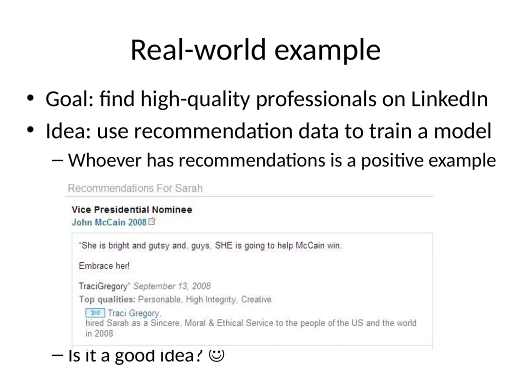
slide20. Real-world example Goal: find high-quality professionals on LinkedIn
Idea: use recommendation data to train a model
Whoever has recommendations is a positive example

Is it a good idea?  
slide21. Not enough (clean) training data? Use existing labels as a guidance rather than a directive
In a semi-supervised clustering framework
Or label more data! 
With a little help from the crowd 
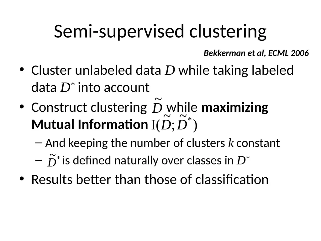
slide22. Semi-supervised clustering Cluster unlabeled data D while taking labeled data D* into account
Construct clustering while maximizing Mutual Information
And keeping the number of clusters k constant
is defined naturally over classes in D*
Results better than those of classification Bekkerman et al, ECML 2006 
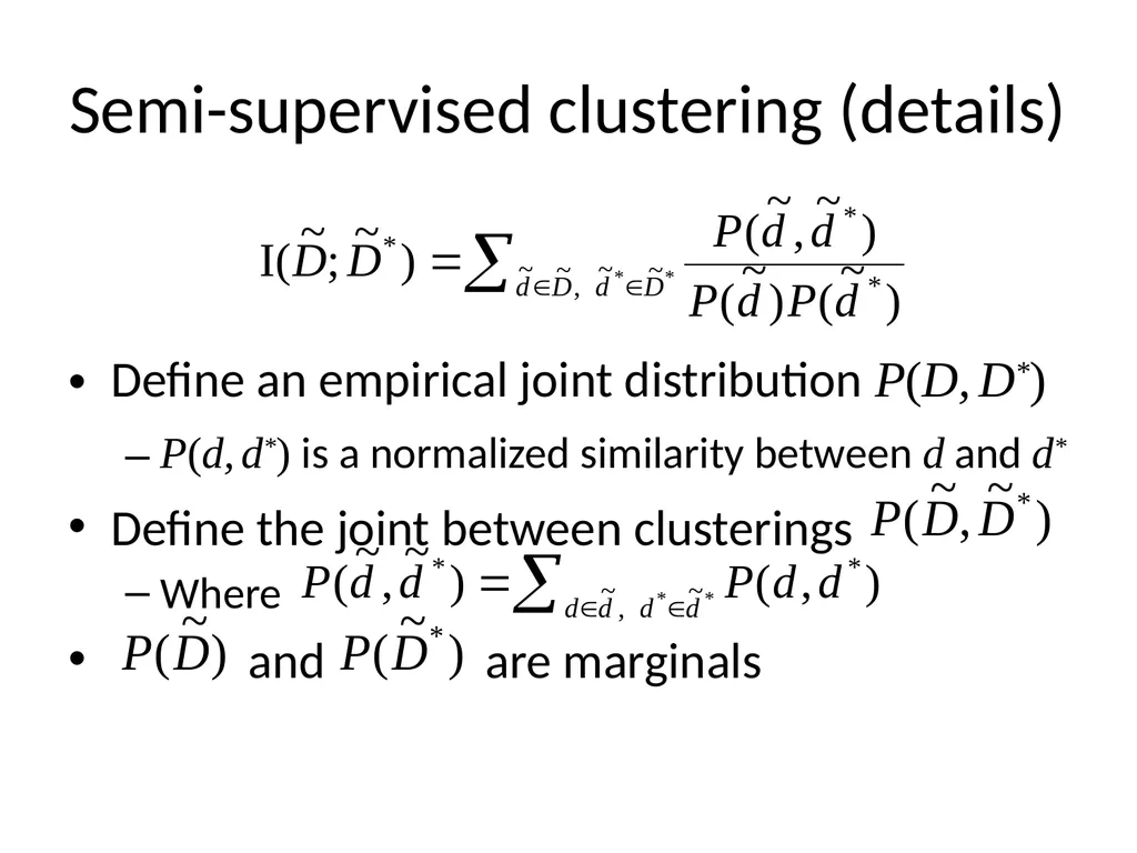
slide23. Semi-supervised clustering (details) Define an empirical joint distribution P(D, D*)
P(d, d*) is a normalized similarity between d and d*
Define the joint between clusterings
Where
and are marginals 
slide24. Crowdsourcing labeled data Crowdsourcing is a tough business 
People are not machines
Any worker who can game the system will game the system
Validation framework + qualification tests are a must
Labeling a lot of data can be fairly expensive 
slide25. How to label 1M instances Budget a month of work + about $50,000 
slide26. How to label 1M instances Hire a data annotation contractor in your town
Presumably someone you know well enough 
slide27. How to label 1M instances Offer the guy $10,000 for one month of work 
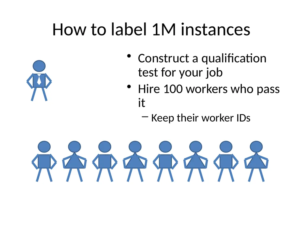
slide28. How to label 1M instances Construct a qualification test for your job
Hire 100 workers who pass it
Keep their worker IDs 
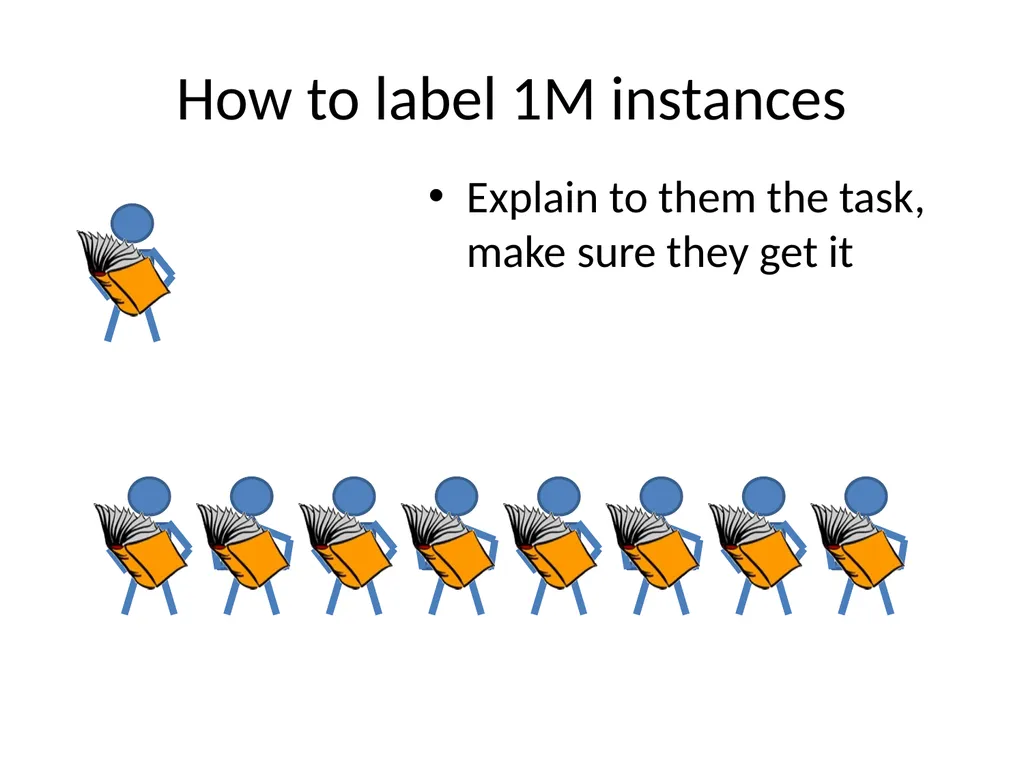
slide29. How to label 1M instances Explain to them the task, make sure they get it 
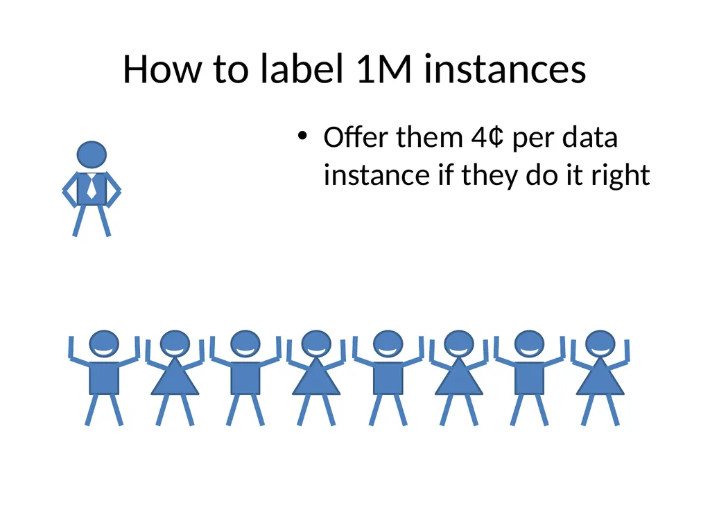
slide30. How to label 1M instances Offer them 4¢ per data instance if they do it right 
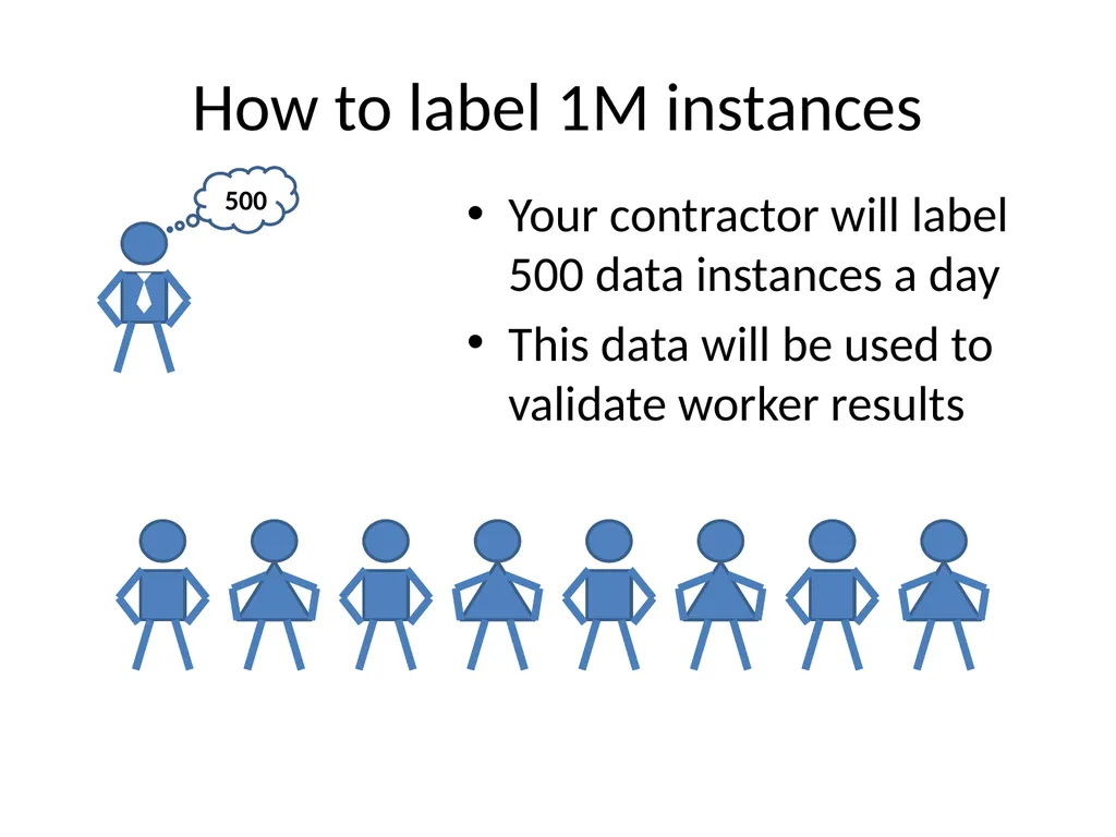
slide31. How to label 1M instances Your contractor will label 500 data instances a day
This data will be used to validate worker results 500 
slide32. How to label 1M instances You’ll need to spot-check the results 
slide33. How to label 1M instances You’ll need to spot-check the results 
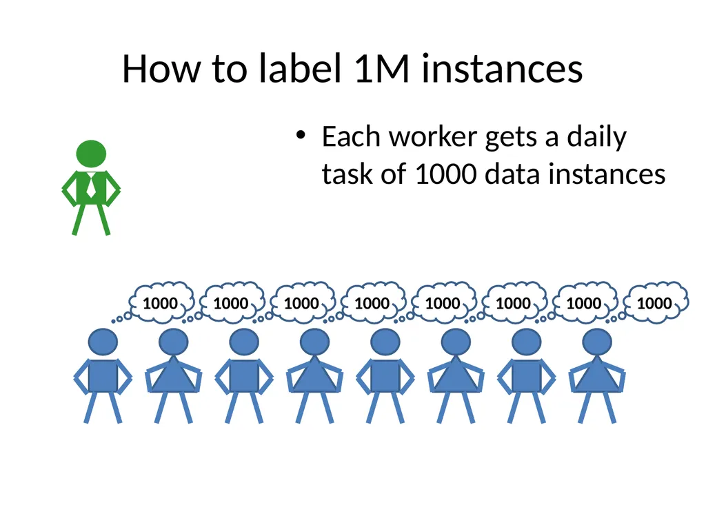
slide34. How to label 1M instances Each worker gets a daily task of 1000 data instances 1000 1000 1000 1000 1000 1000 1000 1000 
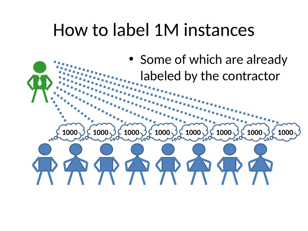
slide35. How to label 1M instances Some of which are already labeled by the contractor 1000 1000 1000 1000 1000 1000 1000 1000 
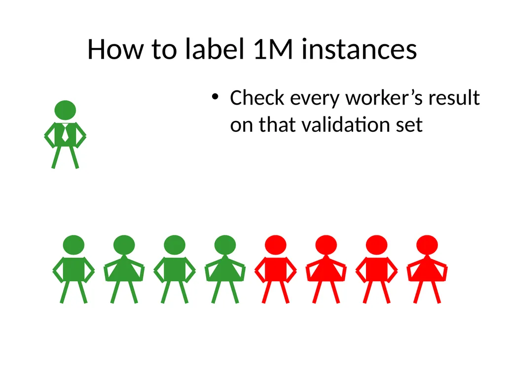
slide36. How to label 1M instances Check every worker’s result on that validation set 
slide37. How to label 1M instances Check every worker’s result on that validation set 
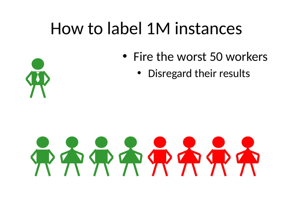
slide38. How to label 1M instances Fire the worst 50 workers
Disregard their results 
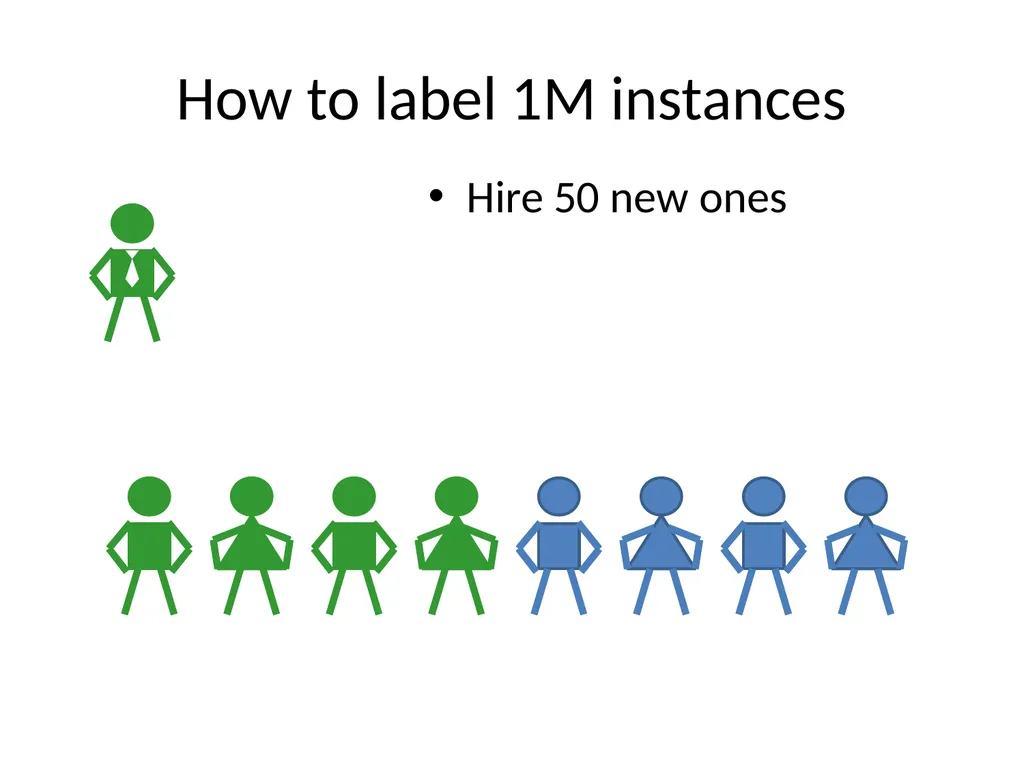
slide39. How to label 1M instances Hire 50 new ones 
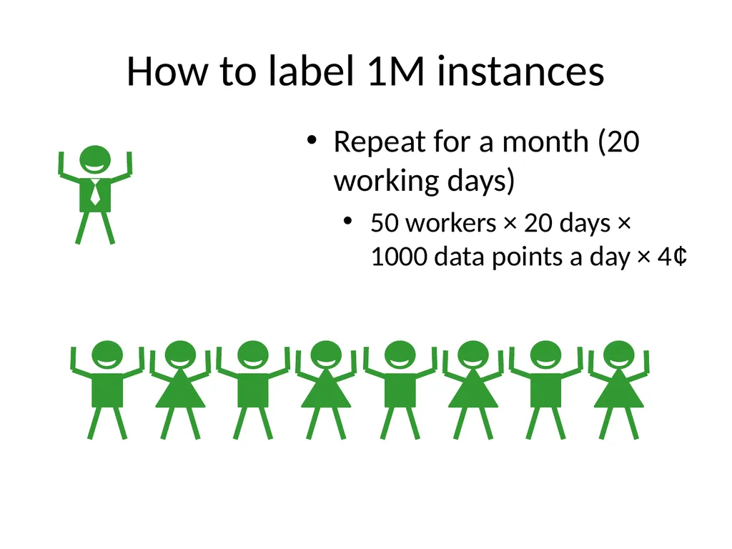
slide40. How to label 1M instances Repeat for a month (20 working days)
50 workers × 20 days × 1000 data points a day × 4¢ 
slide41. Got 1M labeled instances, now what? Now go train your model 
Rule of the thumb: heavier algorithms produce better results
Rule of the other thumb: forget about super-quadratic algorithms

Parallelization looks unavoidable 
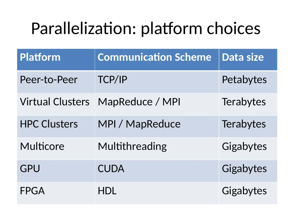
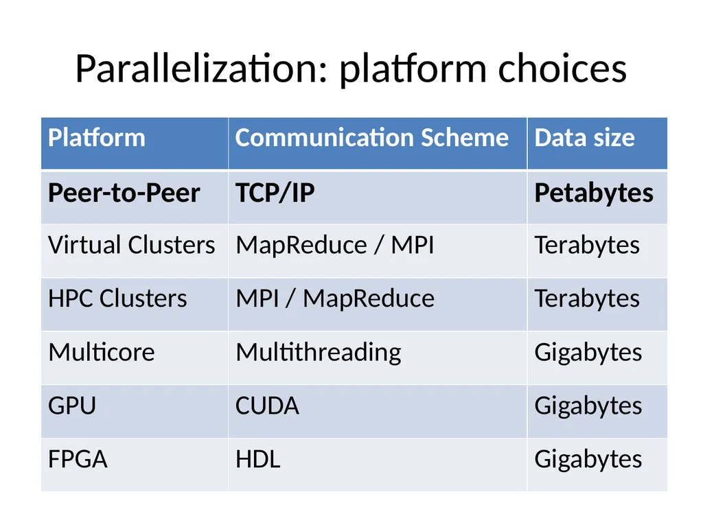
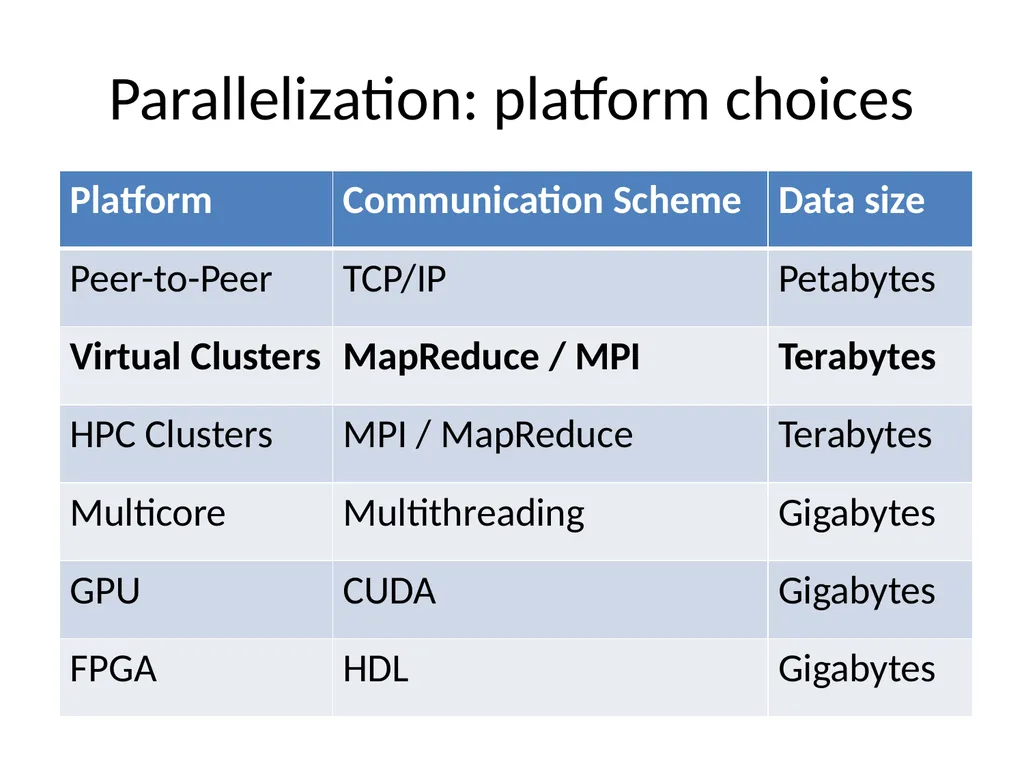
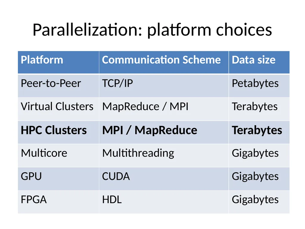
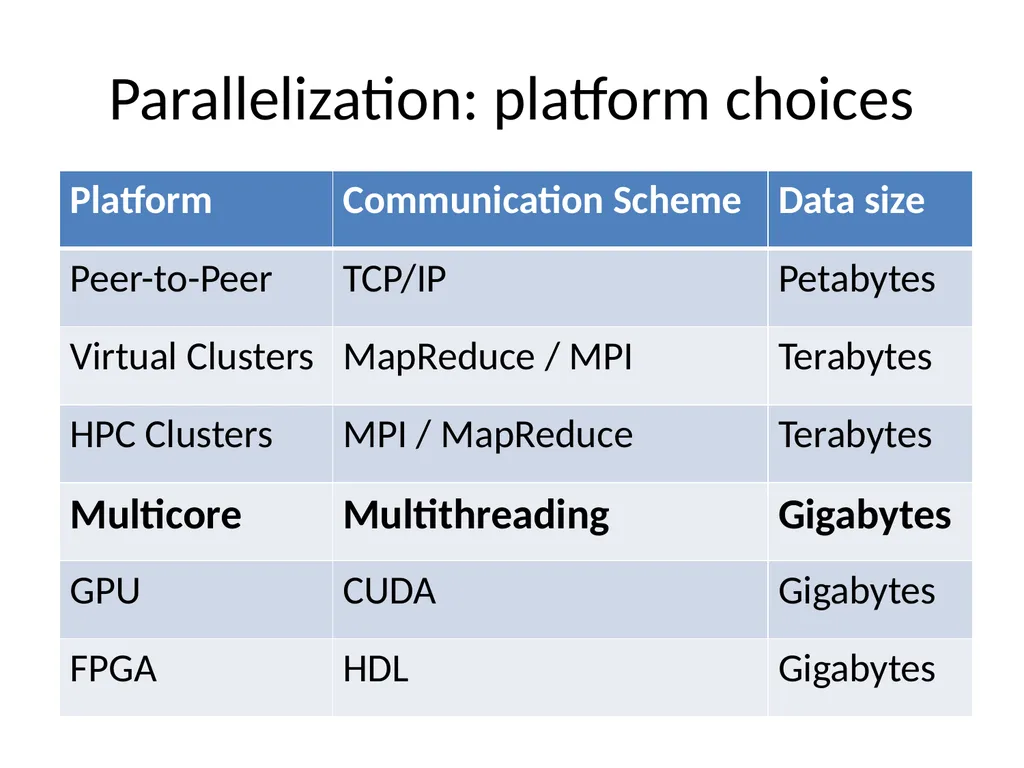
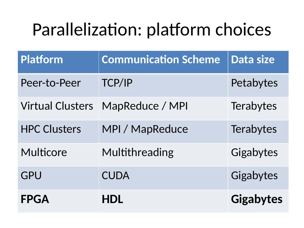
slide42. Parallelization: platform choices 
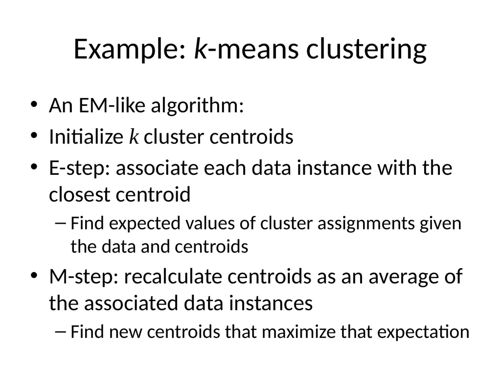
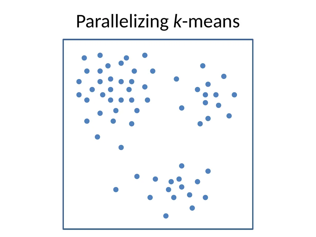
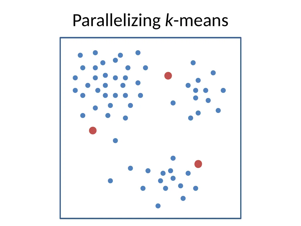
slide43. Example: k-means clustering An EM-like algorithm:
Initialize k cluster centroids
E-step: associate each data instance with the closest centroid
Find expected values of cluster assignments given the data and centroids
M-step: recalculate centroids as an average of the associated data instances
Find new centroids that maximize that expectation 
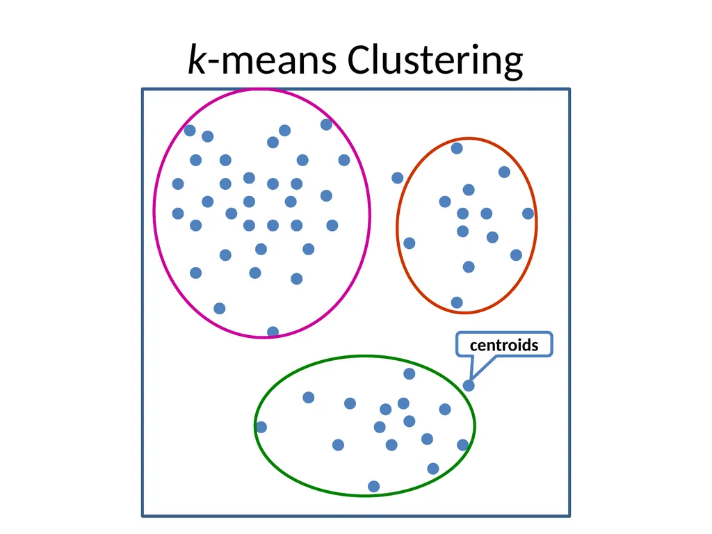
slide44. k-means Clustering centroids 
slide45. Parallelizing k-means 
slide46. Parallelizing k-means 
slide47. Parallelizing k-means 
slide48. Parallelization: platform choices 
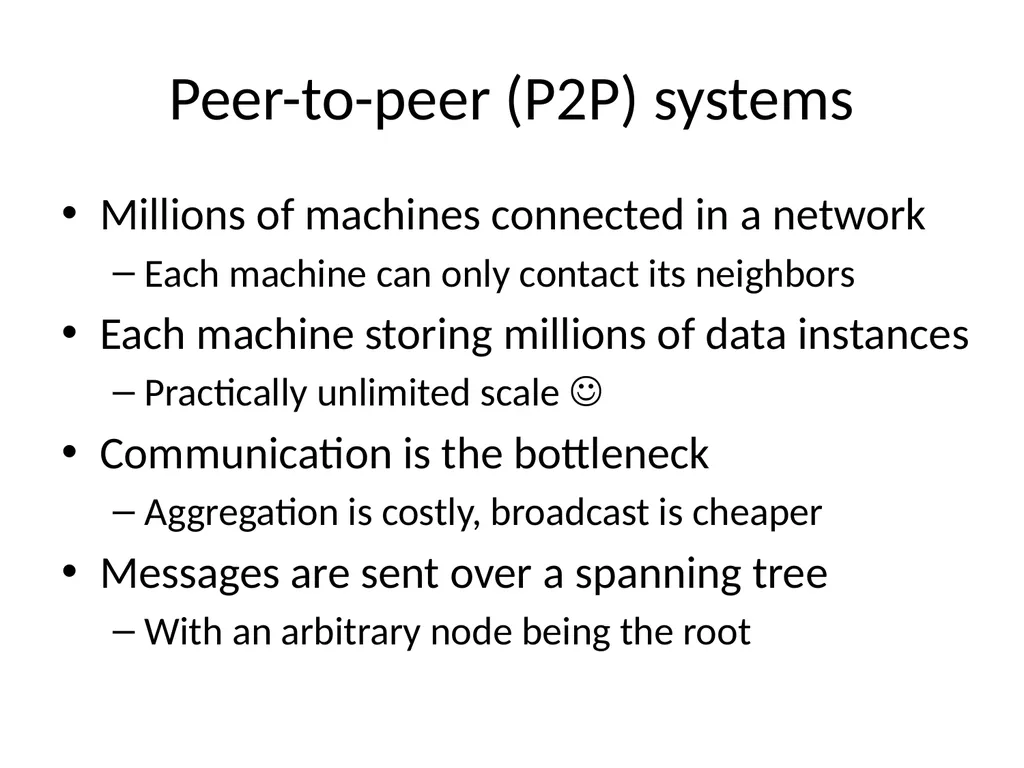
slide49. Peer-to-peer (P2P) systems Millions of machines connected in a network
Each machine can only contact its neighbors
Each machine storing millions of data instances
Practically unlimited scale 
Communication is the bottleneck
Aggregation is costly, broadcast is cheaper
Messages are sent over a spanning tree
With an arbitrary node being the root 
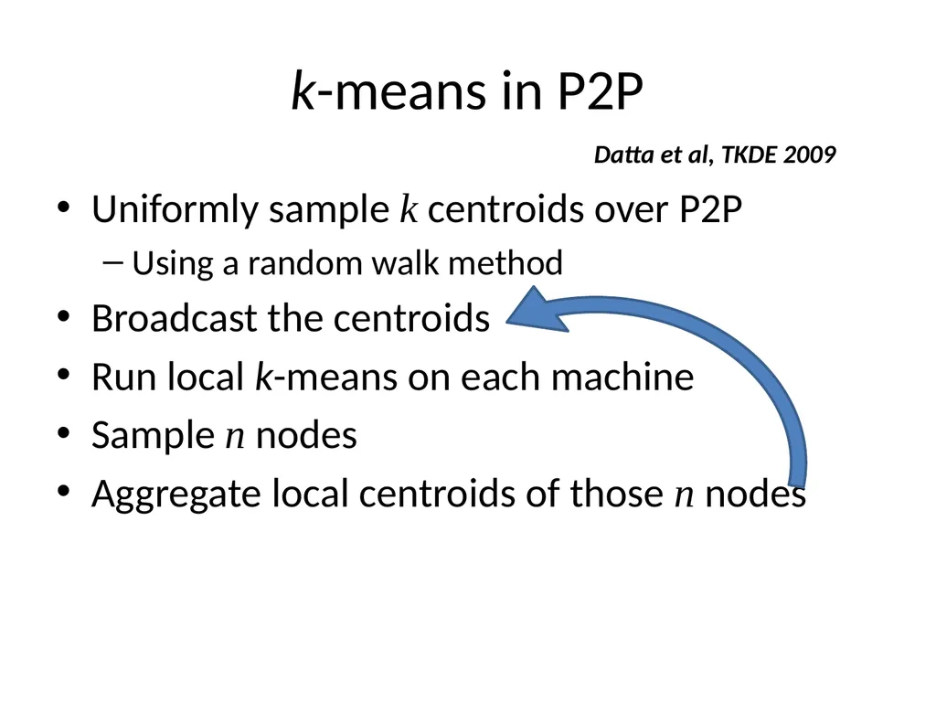
slide50. k-means in P2P Uniformly sample k centroids over P2P
Using a random walk method
Broadcast the centroids
Run local k-means on each machine
Sample n nodes
Aggregate local centroids of those n nodes Datta et al, TKDE 2009 
slide51. Parallelization: platform choices 
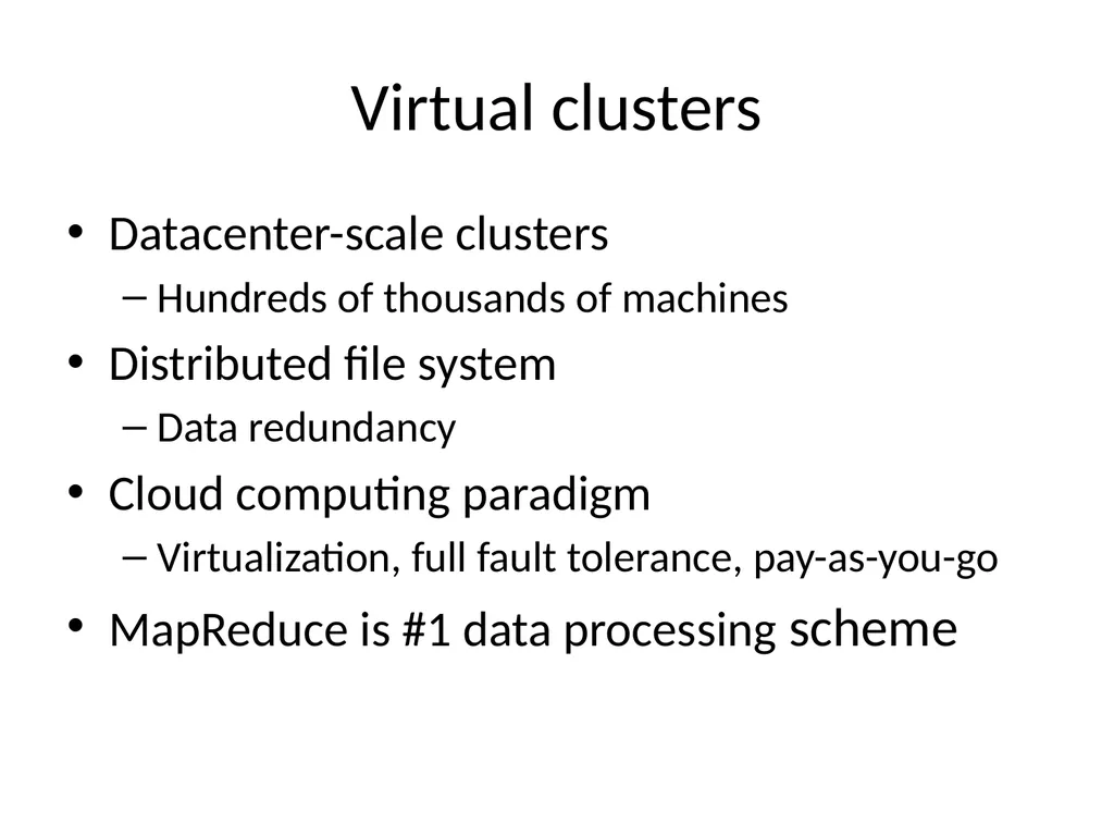
slide52. Virtual clusters Datacenter-scale clusters
Hundreds of thousands of machines
Distributed file system
Data redundancy
Cloud computing paradigm
Virtualization, full fault tolerance, pay-as-you-go
MapReduce is #1 data processing scheme 
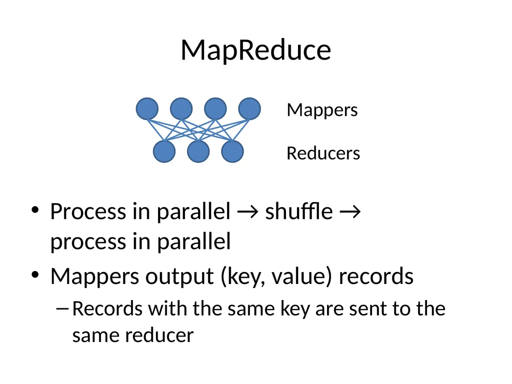
slide53. MapReduce Mappers Reducers Process in parallel → shuffle → process in parallel
Mappers output (key, value) records
Records with the same key are sent to the same reducer 
slide54. MapReduce Example: count words Given 1B docs, what are global word counts?
Split the dataset to portions
Mapper:
Over one data portion, compute local word counts
Output (word, count) pairs – words are the keys
Reducer:
Aggregate local word counts into global ones 
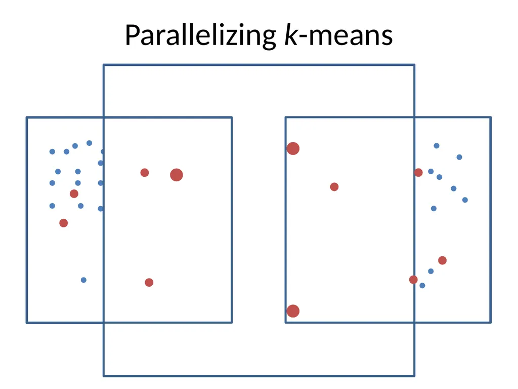
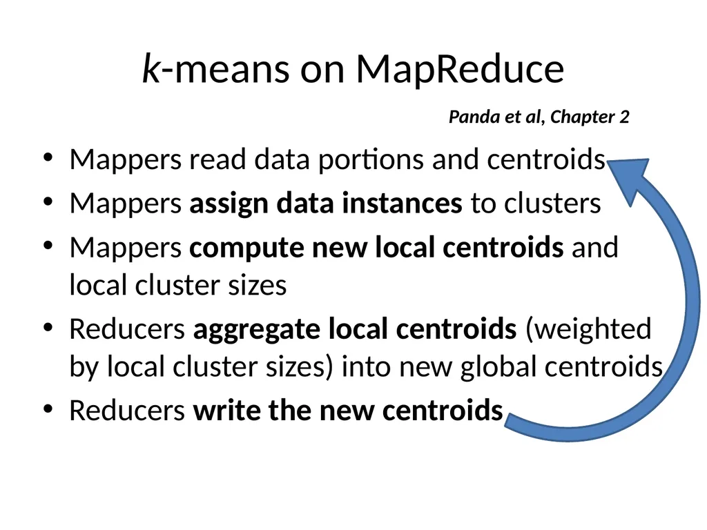
slide55. k-means on MapReduce Mappers read data portions and centroids
Mappers assign data instances to clusters
Mappers compute new local centroids and local cluster sizes
Reducers aggregate local centroids (weighted by local cluster sizes) into new global centroids
Reducers write the new centroids Panda et al, Chapter 2 
slide56. Discussion on MapReduce MapReduce is not designed for iterative processing
Mappers read the same data again and again
MapReduce looks too low-level to some people
Data analysts are traditionally SQL folks 
MapReduce looks too high-level to others
A lot of MapReduce logic is hard to adapt
Example: global word counts 
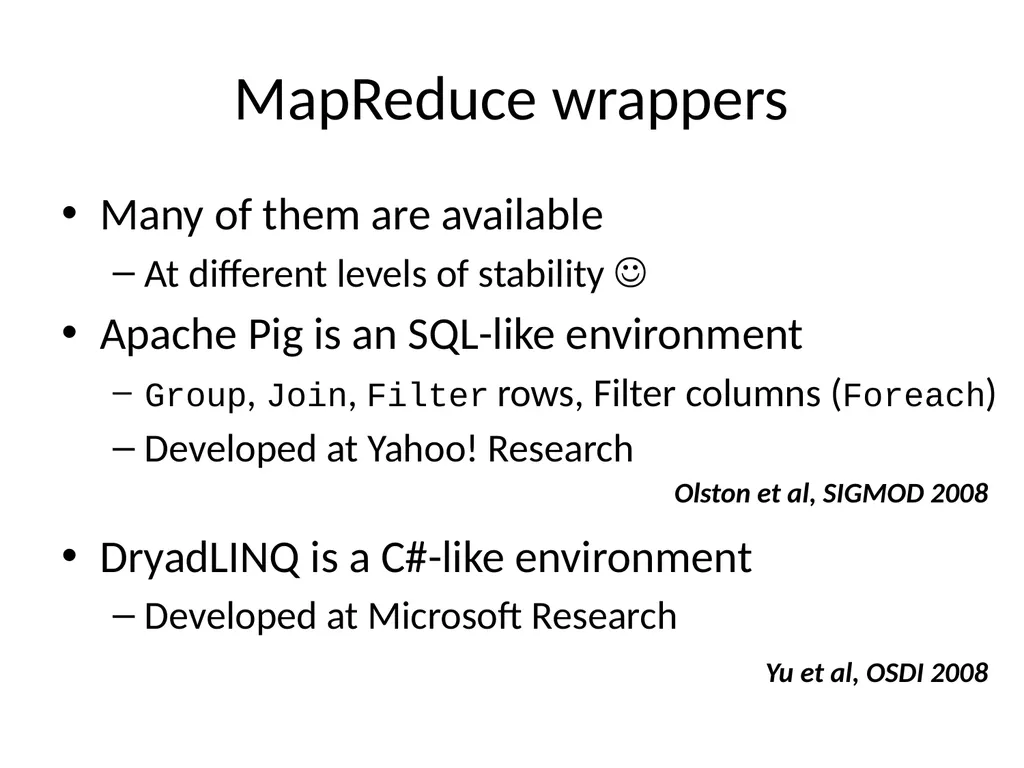
slide57. MapReduce wrappers Many of them are available
At different levels of stability 
Apache Pig is an SQL-like environment
Group, Join, Filter rows, Filter columns (Foreach)
Developed at Yahoo! Research

DryadLINQ is a C#-like environment
Developed at Microsoft Research Olston et al, SIGMOD 2008 Yu et al, OSDI 2008 
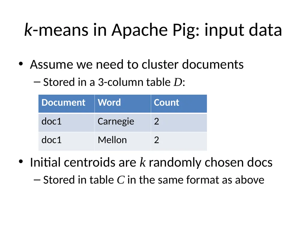
slide58. k-means in Apache Pig: input data Assume we need to cluster documents
Stored in a 3-column table D:

Initial centroids are k randomly chosen docs
Stored in table C in the same format as above 
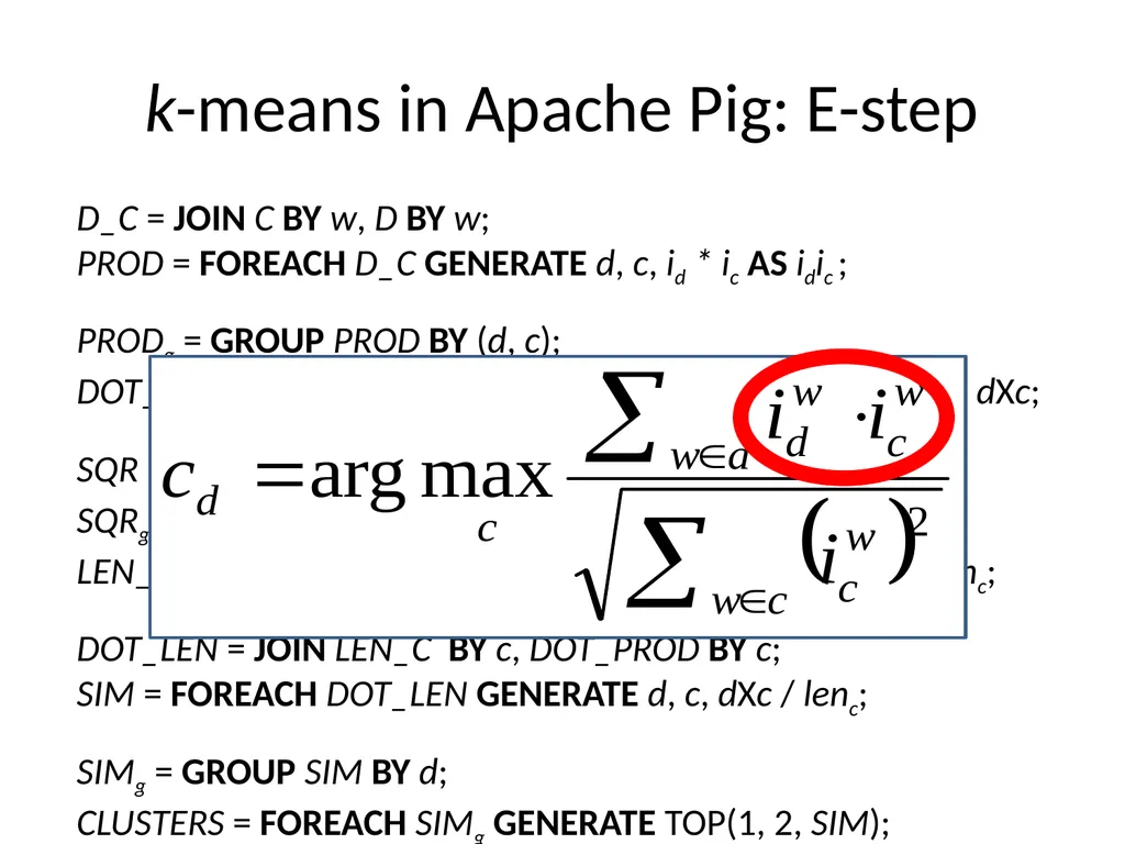
slide59. D_C = JOIN C BY w, D BY w;
PROD = FOREACH D_C GENERATE d, c, id * ic AS idic ;

PRODg = GROUP PROD BY (d, c);
DOT_PROD = FOREACH PRODg GENERATE d, c, SUM(idic) AS dXc;

SQR = FOREACH C GENERATE c, ic * ic AS ic2;
SQRg = GROUP SQR BY c;
LEN_C = FOREACH SQRg GENERATE c, SQRT(SUM(ic2)) AS lenc;

DOT_LEN = JOIN LEN_C BY c, DOT_PROD BY c;
SIM = FOREACH DOT_LEN GENERATE d, c, dXc / lenc;

SIMg = GROUP SIM BY d;
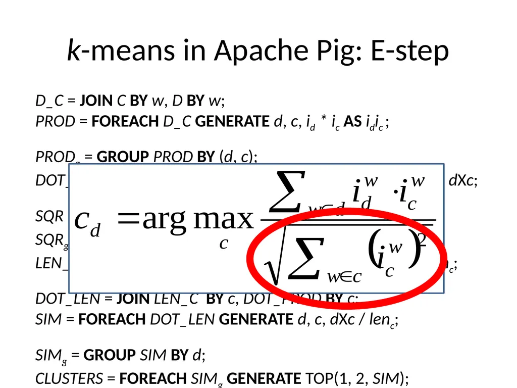
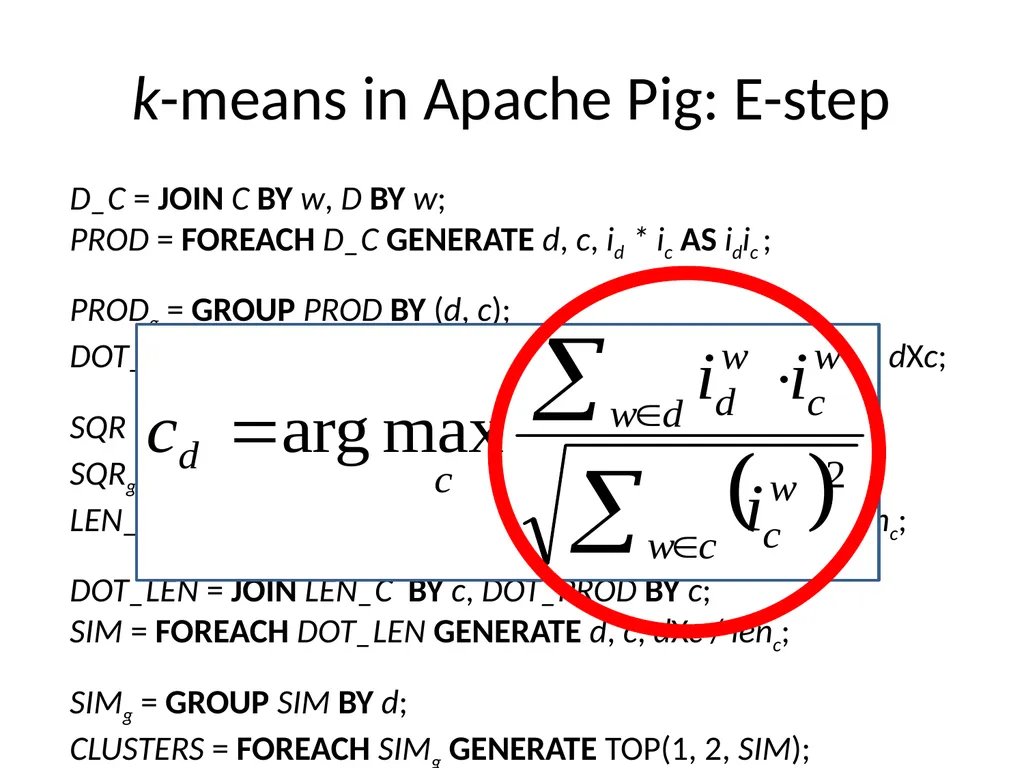
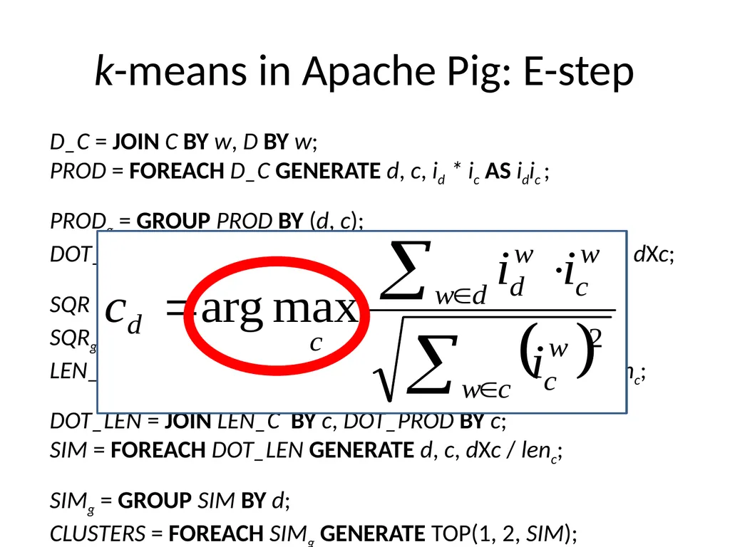
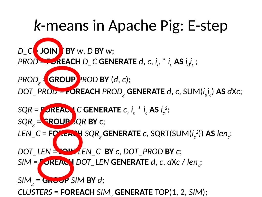
CLUSTERS = FOREACH SIMg GENERATE TOP(1, 2, SIM); k-means in Apache Pig: E-step 
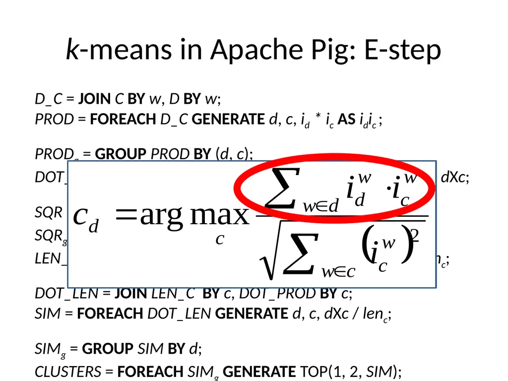
slide60. D_C = JOIN C BY w, D BY w;
PROD = FOREACH D_C GENERATE d, c, id * ic AS idic ;

PRODg = GROUP PROD BY (d, c);
DOT_PROD = FOREACH PRODg GENERATE d, c, SUM(idic) AS dXc;

SQR = FOREACH C GENERATE c, ic * ic AS ic2;
SQRg = GROUP SQR BY c;
LEN_C = FOREACH SQRg GENERATE c, SQRT(SUM(ic2)) AS lenc;

DOT_LEN = JOIN LEN_C BY c, DOT_PROD BY c;
SIM = FOREACH DOT_LEN GENERATE d, c, dXc / lenc;

SIMg = GROUP SIM BY d;
CLUSTERS = FOREACH SIMg GENERATE TOP(1, 2, SIM); k-means in Apache Pig: E-step 
slide61. D_C = JOIN C BY w, D BY w;
PROD = FOREACH D_C GENERATE d, c, id * ic AS idic ;

PRODg = GROUP PROD BY (d, c);
DOT_PROD = FOREACH PRODg GENERATE d, c, SUM(idic) AS dXc;

SQR = FOREACH C GENERATE c, ic * ic AS ic2;
SQRg = GROUP SQR BY c;
LEN_C = FOREACH SQRg GENERATE c, SQRT(SUM(ic2)) AS lenc;

DOT_LEN = JOIN LEN_C BY c, DOT_PROD BY c;
SIM = FOREACH DOT_LEN GENERATE d, c, dXc / lenc;

SIMg = GROUP SIM BY d;
CLUSTERS = FOREACH SIMg GENERATE TOP(1, 2, SIM); k-means in Apache Pig: E-step 
slide62. D_C = JOIN C BY w, D BY w;
PROD = FOREACH D_C GENERATE d, c, id * ic AS idic ;

PRODg = GROUP PROD BY (d, c);
DOT_PROD = FOREACH PRODg GENERATE d, c, SUM(idic) AS dXc;

SQR = FOREACH C GENERATE c, ic * ic AS ic2;
SQRg = GROUP SQR BY c;
LEN_C = FOREACH SQRg GENERATE c, SQRT(SUM(ic2)) AS lenc;

DOT_LEN = JOIN LEN_C BY c, DOT_PROD BY c;
SIM = FOREACH DOT_LEN GENERATE d, c, dXc / lenc;

SIMg = GROUP SIM BY d;
CLUSTERS = FOREACH SIMg GENERATE TOP(1, 2, SIM); k-means in Apache Pig: E-step 
slide63. D_C = JOIN C BY w, D BY w;
PROD = FOREACH D_C GENERATE d, c, id * ic AS idic ;

PRODg = GROUP PROD BY (d, c);
DOT_PROD = FOREACH PRODg GENERATE d, c, SUM(idic) AS dXc;

SQR = FOREACH C GENERATE c, ic * ic AS ic2;
SQRg = GROUP SQR BY c;
LEN_C = FOREACH SQRg GENERATE c, SQRT(SUM(ic2)) AS lenc;

DOT_LEN = JOIN LEN_C BY c, DOT_PROD BY c;
SIM = FOREACH DOT_LEN GENERATE d, c, dXc / lenc;

SIMg = GROUP SIM BY d;
CLUSTERS = FOREACH SIMg GENERATE TOP(1, 2, SIM); k-means in Apache Pig: E-step 
slide64. k-means in Apache Pig: E-step D_C = JOIN C BY w, D BY w;
PROD = FOREACH D_C GENERATE d, c, id * ic AS idic ;

PRODg = GROUP PROD BY (d, c);
DOT_PROD = FOREACH PRODg GENERATE d, c, SUM(idic) AS dXc;

SQR = FOREACH C GENERATE c, ic * ic AS ic2;
SQRg = GROUP SQR BY c;
LEN_C = FOREACH SQRg GENERATE c, SQRT(SUM(ic2)) AS lenc;

DOT_LEN = JOIN LEN_C BY c, DOT_PROD BY c;
SIM = FOREACH DOT_LEN GENERATE d, c, dXc / lenc;

SIMg = GROUP SIM BY d;
CLUSTERS = FOREACH SIMg GENERATE TOP(1, 2, SIM); 
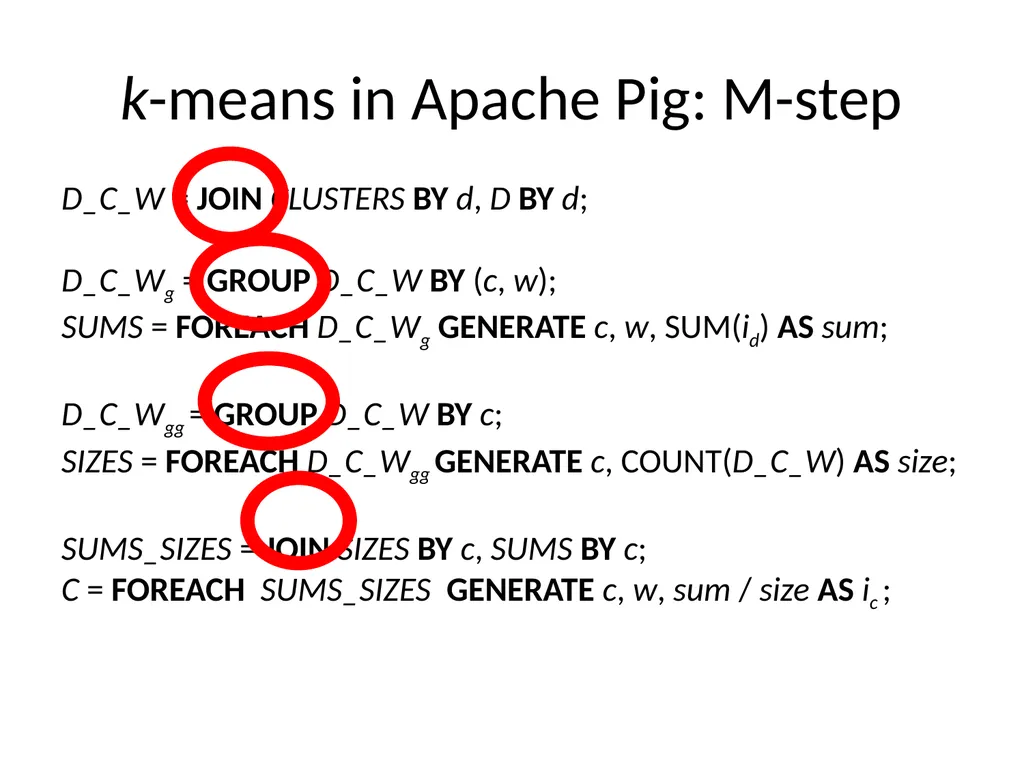
slide65. k-means in Apache Pig: M-step D_C_W = JOIN CLUSTERS BY d, D BY d;

D_C_Wg = GROUP D_C_W BY (c, w);
SUMS = FOREACH D_C_Wg GENERATE c, w, SUM(id) AS sum;

D_C_Wgg = GROUP D_C_W BY c;
SIZES = FOREACH D_C_Wgg GENERATE c, COUNT(D_C_W) AS size;

SUMS_SIZES = JOIN SIZES BY c, SUMS BY c;
C = FOREACH SUMS_SIZES GENERATE c, w, sum / size AS ic ; 
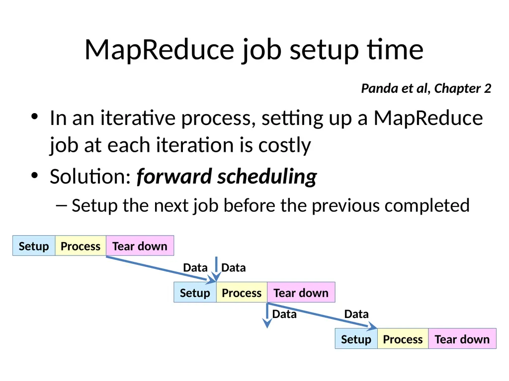
slide66. MapReduce job setup time In an iterative process, setting up a MapReduce job at each iteration is costly
Solution: forward scheduling
Setup the next job before the previous completed Panda et al, Chapter 2 Data Data Data Data 
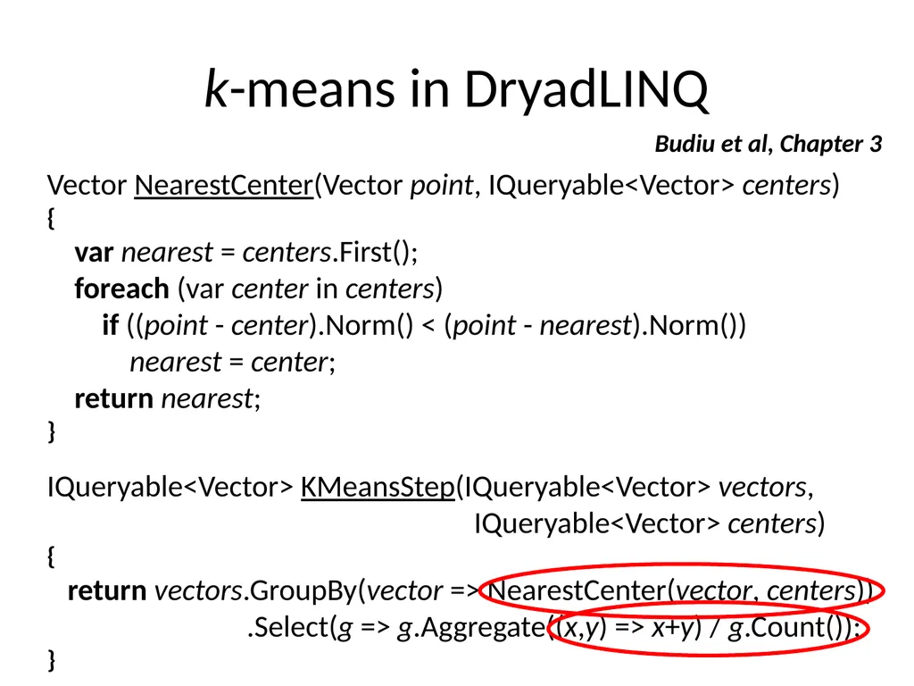
slide67. k-means in DryadLINQ Vector NearestCenter(Vector point, IQueryable<Vector> centers)
{
var nearest = centers.First();
foreach (var center in centers)
if ((point - center).Norm() < (point - nearest).Norm())
nearest = center;
return nearest;
}

IQueryable<Vector> KMeansStep(IQueryable<Vector> vectors,
IQueryable<Vector> centers)
{
return vectors.GroupBy(vector => NearestCenter(vector, centers))
.Select(g => g.Aggregate((x,y) => x+y) / g.Count());
} Budiu et al, Chapter 3 
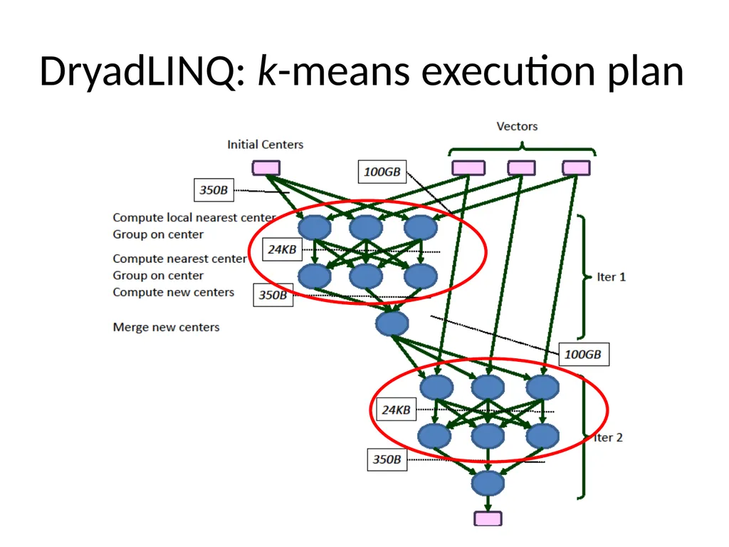
slide68. DryadLINQ: k-means execution plan 
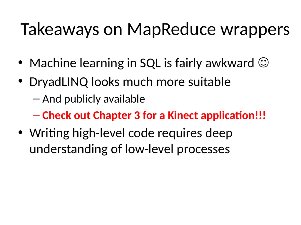
slide69. Takeaways on MapReduce wrappers Machine learning in SQL is fairly awkward 
DryadLINQ looks much more suitable
And publicly available
Check out Chapter 3 for a Kinect application!!!
Writing high-level code requires deep understanding of low-level processes 
slide70. Parallelization: platform choices 
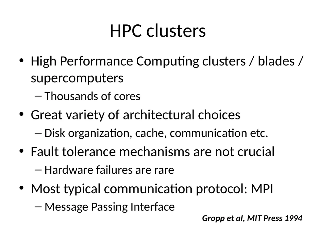
slide71. HPC clusters High Performance Computing clusters / blades / supercomputers
Thousands of cores
Great variety of architectural choices
Disk organization, cache, communication etc.
Fault tolerance mechanisms are not crucial
Hardware failures are rare
Most typical communication protocol: MPI
Message Passing Interface Gropp et al, MIT Press 1994 
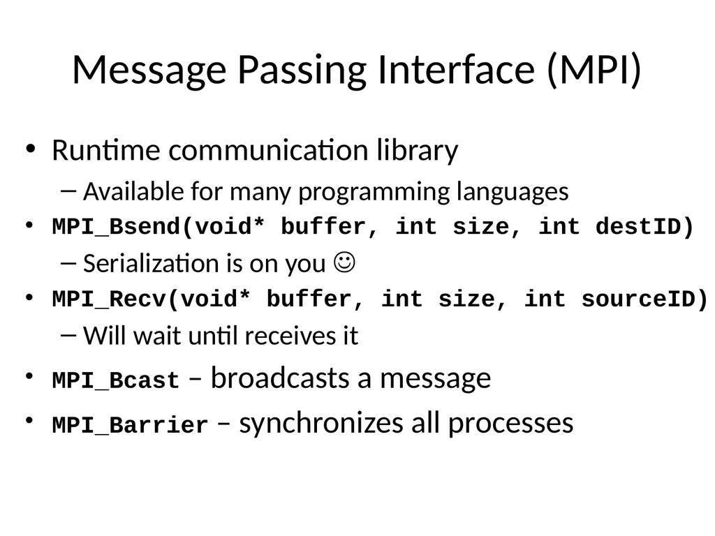
slide72. Message Passing Interface (MPI) Runtime communication library
Available for many programming languages
MPI_Bsend(void* buffer, int size, int destID)
Serialization is on you 
MPI_Recv(void* buffer, int size, int sourceID)
Will wait until receives it
MPI_Bcast – broadcasts a message
MPI_Barrier – synchronizes all processes 
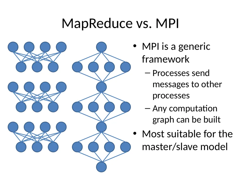
slide73. MapReduce vs. MPI MPI is a generic framework
Processes send messages to other processes
Any computation graph can be built
Most suitable for the master/slave model 
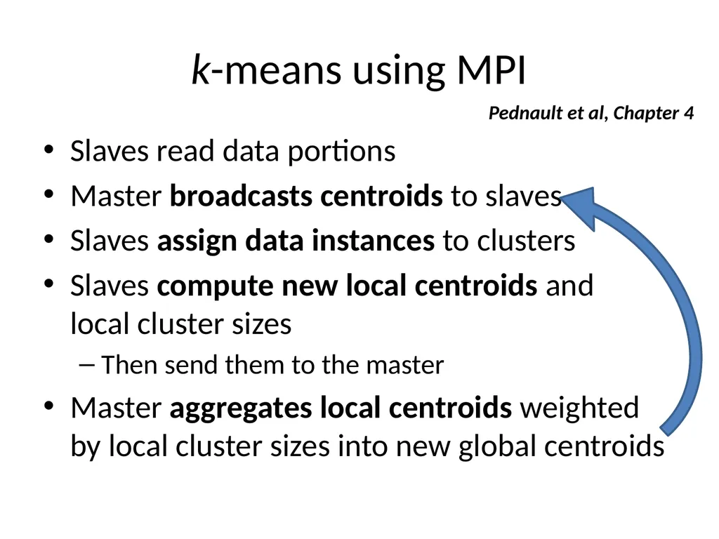
slide74. k-means using MPI Slaves read data portions
Master broadcasts centroids to slaves
Slaves assign data instances to clusters
Slaves compute new local centroids and local cluster sizes
Then send them to the master
Master aggregates local centroids weighted by local cluster sizes into new global centroids Pednault et al, Chapter 4 
slide75. Two features of MPI parallelization State-preserving processes
Processes can live as long as the system runs
No need to read the same data again and again
All necessary parameters can be preserved locally
Hierarchical master/slave paradigm
A slave can be a master of other processes
Could be very useful in dynamic resource allocation
When a slave recognizes it has too much stuff to process Pednault et al, Chapter 4 
slide76. Takeaways on MPI Old, well established, well debugged
Very flexible
Perfectly suitable for iterative processing
Fault intolerant
Not that widely available anymore 
An open source implementation: OpenMPI
MPI can be deployed on Hadoop Ye et al, CIKM 2009 
slide77. Parallelization: platform choices 
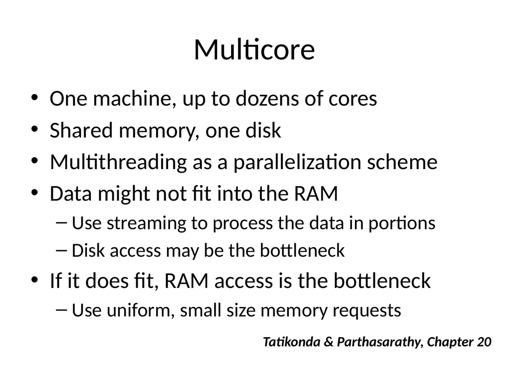
slide78. Multicore One machine, up to dozens of cores
Shared memory, one disk
Multithreading as a parallelization scheme
Data might not fit into the RAM
Use streaming to process the data in portions
Disk access may be the bottleneck
If it does fit, RAM access is the bottleneck
Use uniform, small size memory requests Tatikonda & Parthasarathy, Chapter 20 
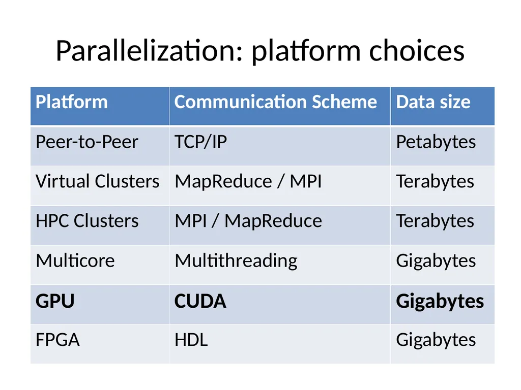
slide79. Parallelization: platform choices 
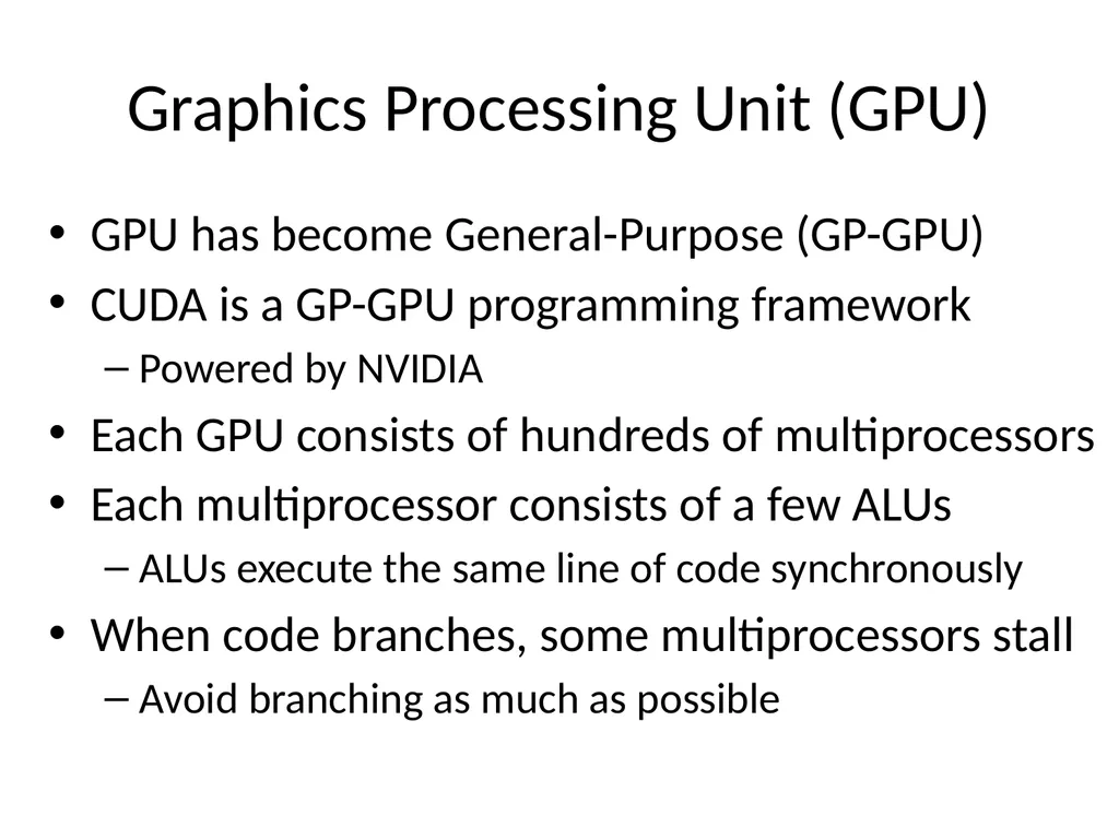
slide80. Graphics Processing Unit (GPU) GPU has become General-Purpose (GP-GPU)
CUDA is a GP-GPU programming framework
Powered by NVIDIA
Each GPU consists of hundreds of multiprocessors
Each multiprocessor consists of a few ALUs
ALUs execute the same line of code synchronously
When code branches, some multiprocessors stall
Avoid branching as much as possible 
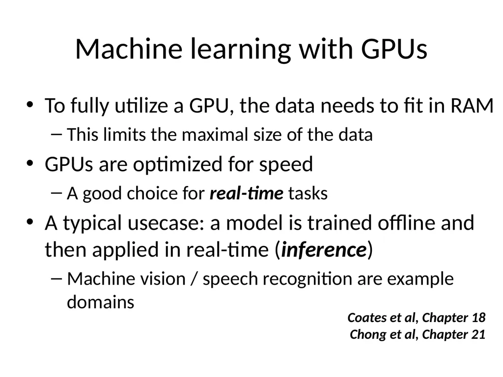
slide81. Machine learning with GPUs To fully utilize a GPU, the data needs to fit in RAM
This limits the maximal size of the data
GPUs are optimized for speed
A good choice for real-time tasks
A typical usecase: a model is trained offline and then applied in real-time (inference)
Machine vision / speech recognition are example domains Coates et al, Chapter 18
Chong et al, Chapter 21 
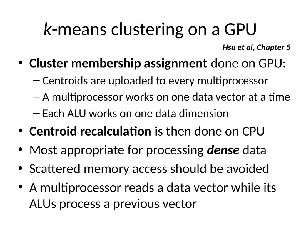
slide82. k-means clustering on a GPU Cluster membership assignment done on GPU:
Centroids are uploaded to every multiprocessor
A multiprocessor works on one data vector at a time
Each ALU works on one data dimension
Centroid recalculation is then done on CPU
Most appropriate for processing dense data
Scattered memory access should be avoided
A multiprocessor reads a data vector while its ALUs process a previous vector Hsu et al, Chapter 5 
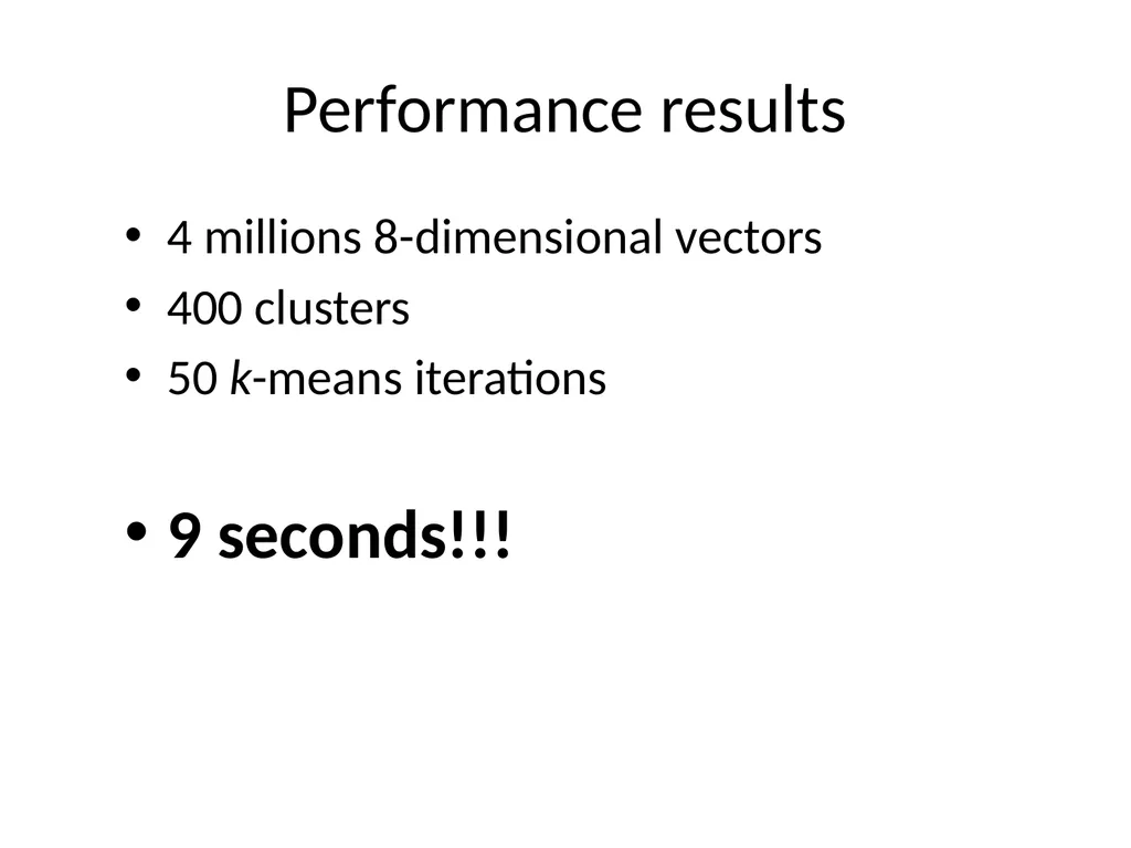
slide83. Performance results 4 millions 8-dimensional vectors
400 clusters
50 k-means iterations

9 seconds!!! 
slide84. Parallelization: platform choices 
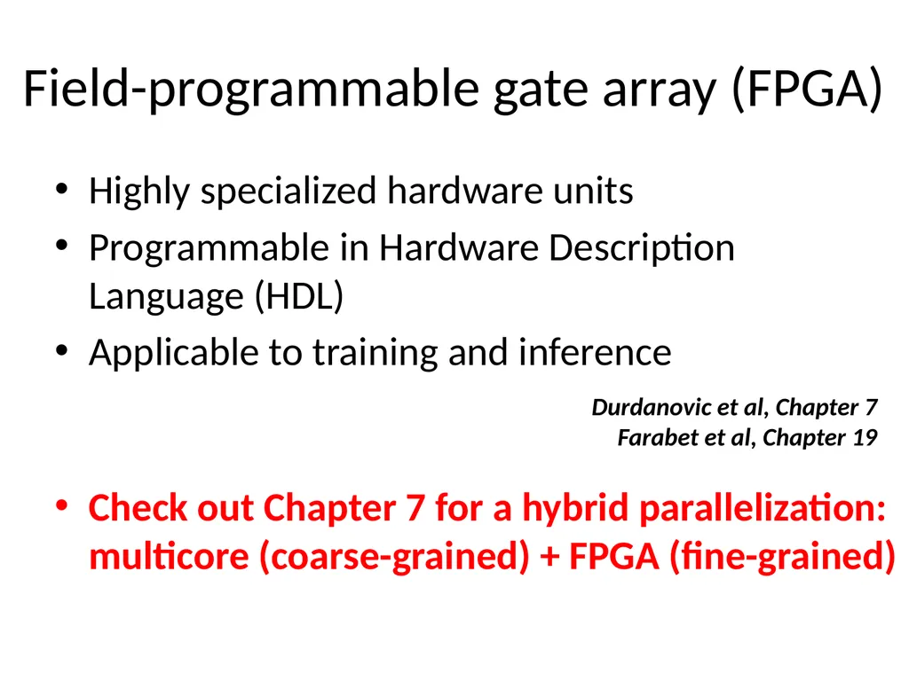
slide85. Field-programmable gate array (FPGA) Highly specialized hardware units
Programmable in Hardware Description Language (HDL)
Applicable to training and inference

Check out Chapter 7 for a hybrid parallelization: multicore (coarse-grained) + FPGA (fine-grained) Durdanovic et al, Chapter 7
Farabet et al, Chapter 19 
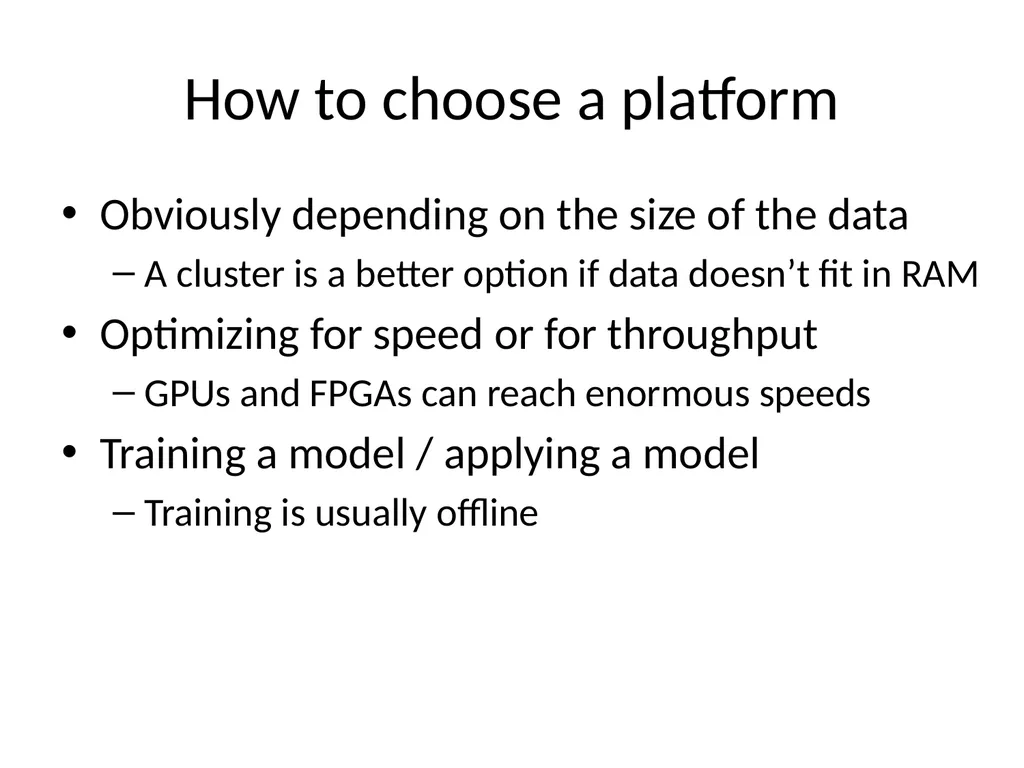
slide86. How to choose a platform Obviously depending on the size of the data
A cluster is a better option if data doesn’t fit in RAM
Optimizing for speed or for throughput
GPUs and FPGAs can reach enormous speeds
Training a model / applying a model
Training is usually offline 
slide87. Thank You! http://hunch.net/~large_scale_survey 
slide88. Parallel Information-Theoretic Co-Clustering Bekkerman & Scholz, Chapter 13 
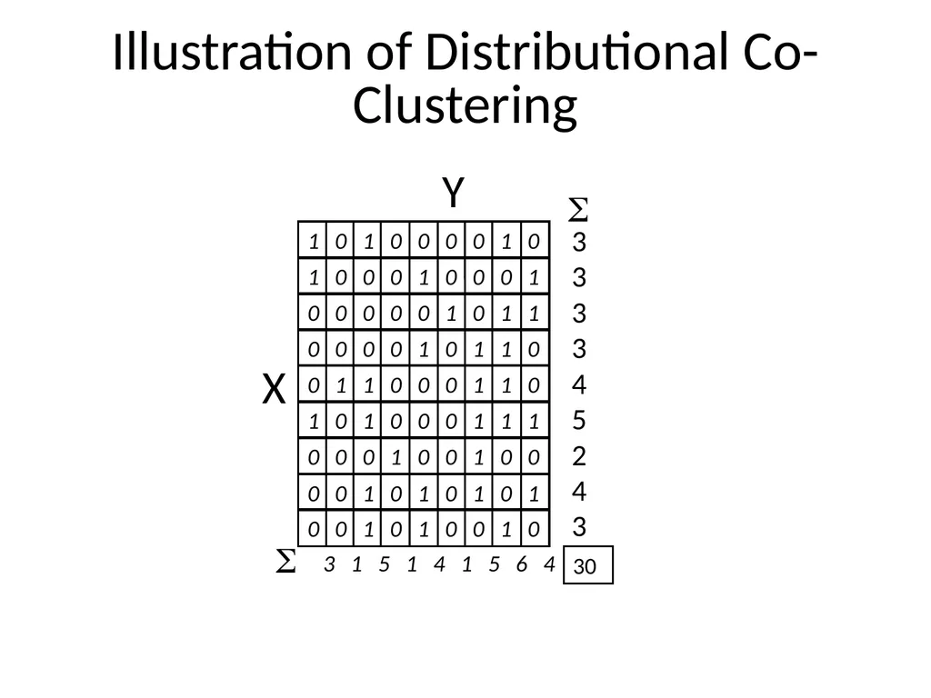
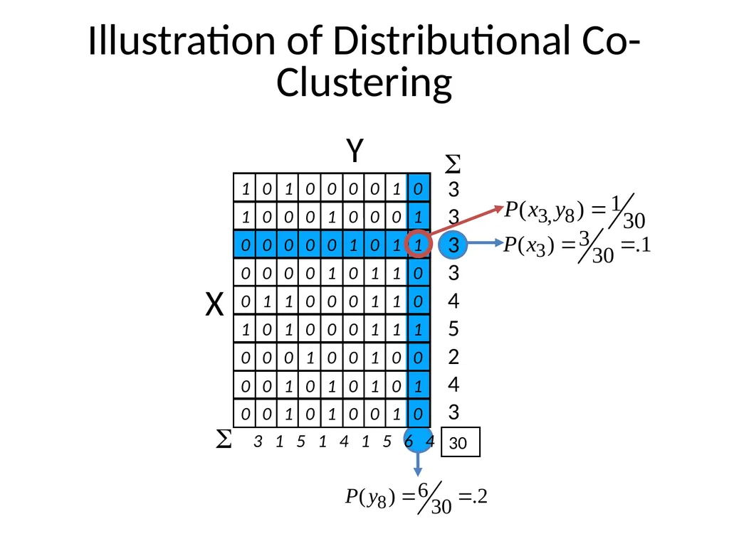
slide89. Illustration of Distributional Co-Clustering 3
3
3
3
4
5
2
4
3 3 1 5 1 4 1 5 6 4 30   X Y 
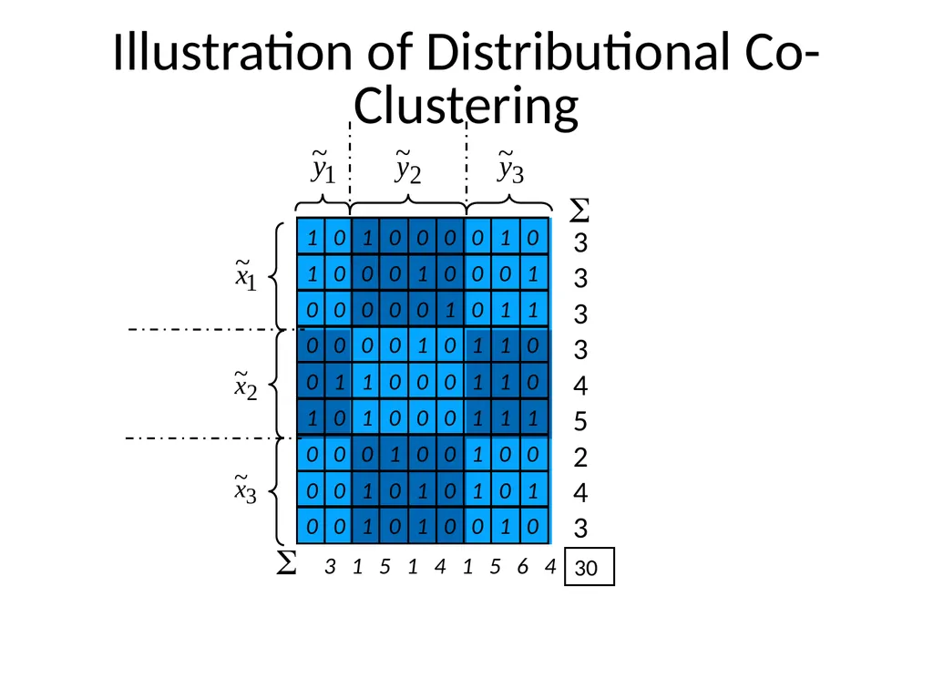
slide90. Illustration of Distributional Co-Clustering 3
3
3
3
4
5
2
4
3 3 1 5 1 4 1 5 6 4 30   X Y 
slide91. Illustration of Distributional Co-Clustering 3
3
3
3
4
5
2
4
3 3 1 5 1 4 1 5 6 4 30   
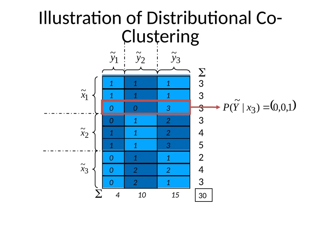
slide92. 0 0 3 4 10 15 Illustration of Distributional Co-Clustering 1 1 1 3
3
3
3
4
5
2
4
3 30   1 1 1 0 1 2 1 1 2 1 1 3 0 1 1 0 2 2 0 2 1 
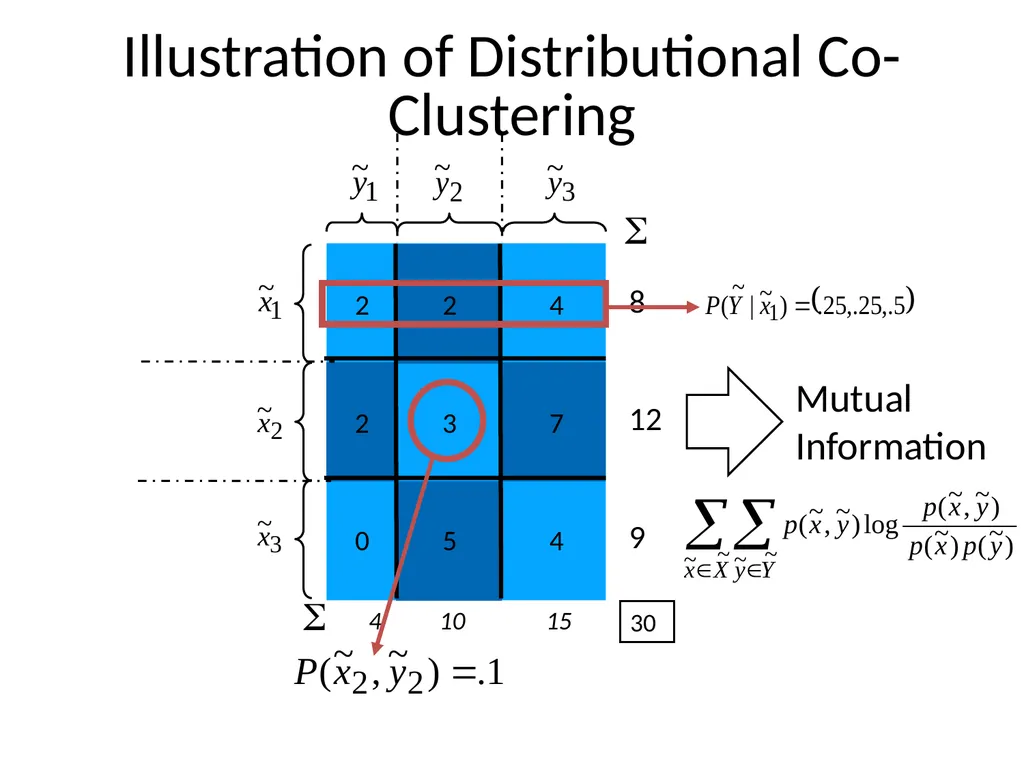
slide93. Illustration of Distributional Co-Clustering 8

12

9 4 10 15 30   2 2 4 2 3 7 0 5 4 
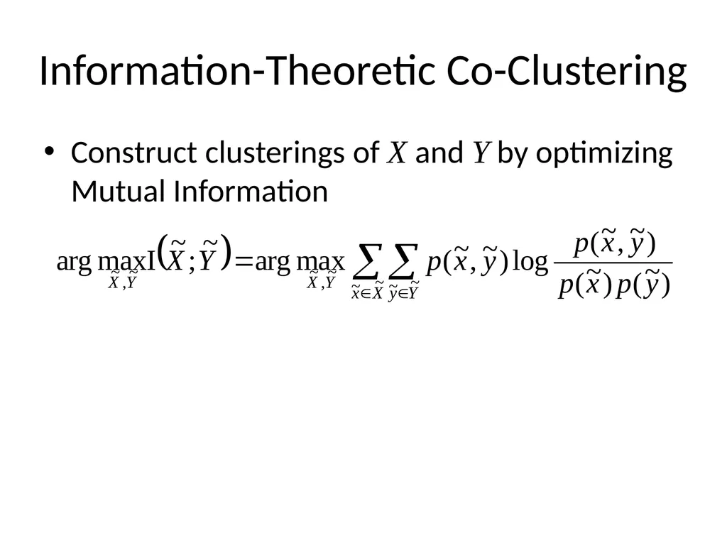
slide94. Information-Theoretic Co-Clustering Construct clusterings of X and Y by optimizing Mutual Information 
slide95. Dhillon et al, KDD 2003 Two optimization strategies Both strategies:
Randomly initialize clusterings of X and Y
Alternate reclustering wrt and wrt
Strategy 1: Centroid-based

At iteration t, assign each x to cluster x with
Compute for each new cluster x ~ ~ 
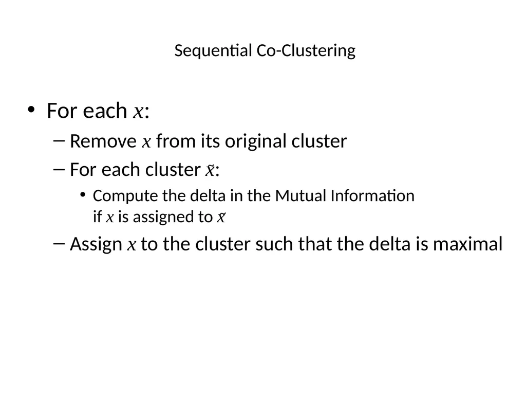
slide96. Sequential Co-Clustering For each x:
Remove x from its original cluster
For each cluster x:
Compute the delta in the Mutual Information if x is assigned to x
Assign x to the cluster such that the delta is maximal ~ ~ 
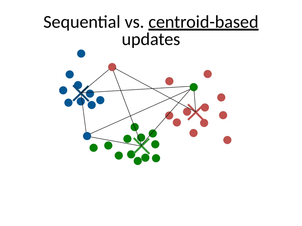
slide97. Sequential vs. centroid-based updates 
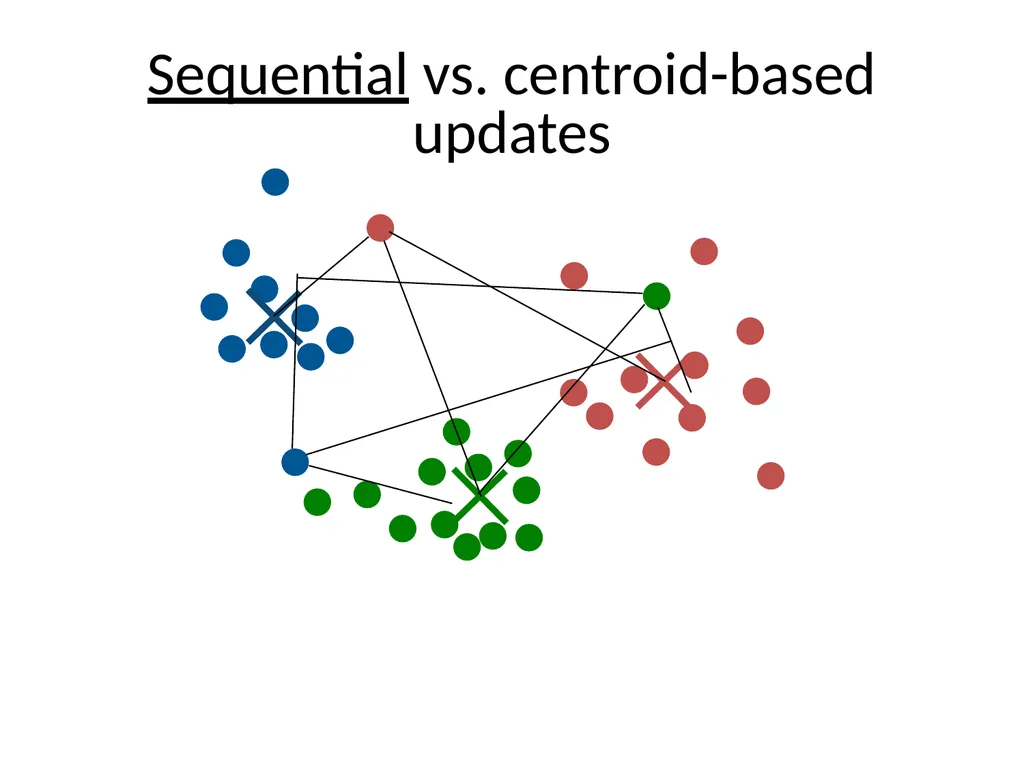
slide98. Sequential vs. centroid-based updates 
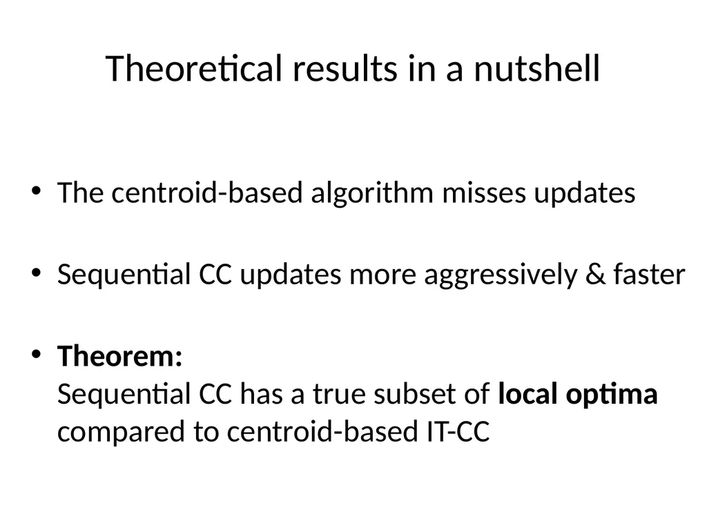
slide99. Theoretical results in a nutshell The centroid-based algorithm misses updates
Sequential CC updates more aggressively & faster
Theorem:Sequential CC has a true subset of local optima compared to centroid-based IT-CC 
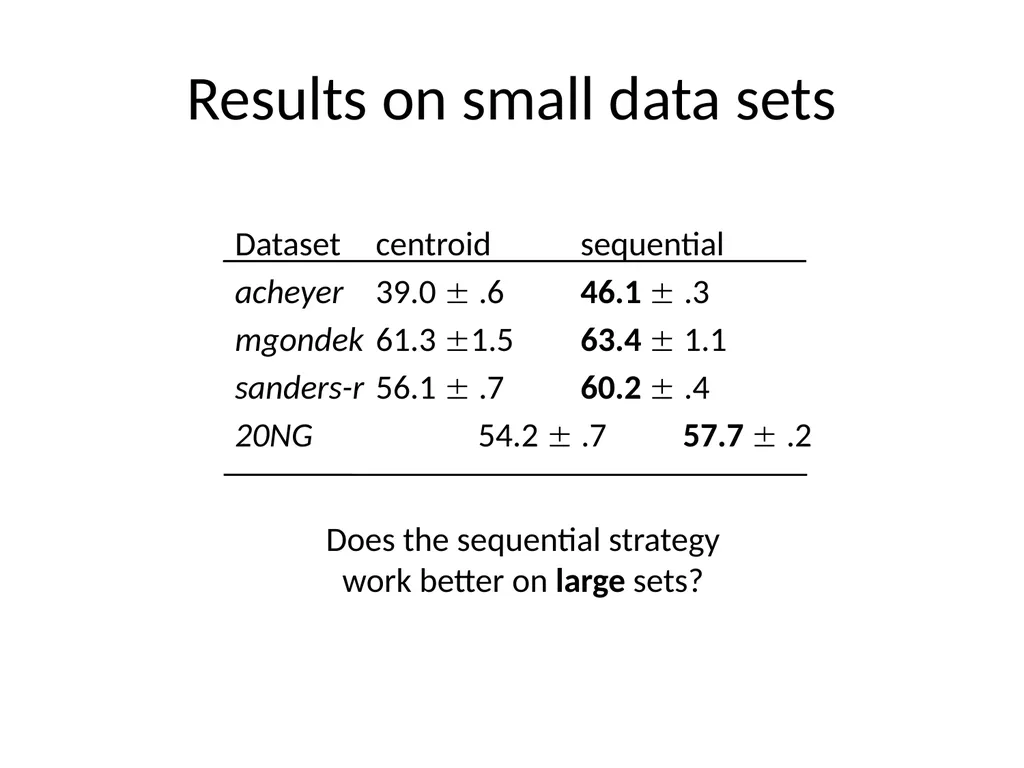
slide100. Results on small data sets Dataset centroid sequential
acheyer 39.0  .6 46.1  .3
mgondek 61.3 1.5 63.4  1.1
sanders-r 56.1  .7 60.2  .4
20NG 54.2  .7 57.7  .2 Does the sequential strategy
work better on large sets? 
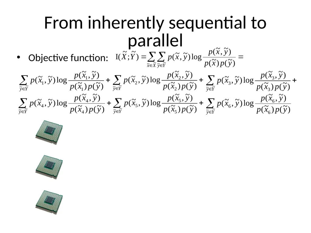
slide101. From inherently sequential to parallel Objective function: 
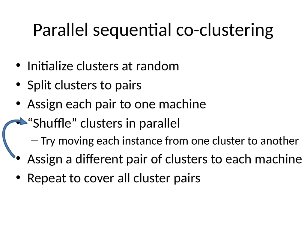
slide102. Parallel sequential co-clustering Initialize clusters at random
Split clusters to pairs
Assign each pair to one machine
“Shuffle” clusters in parallel
Try moving each instance from one cluster to another
Assign a different pair of clusters to each machine
Repeat to cover all cluster pairs 
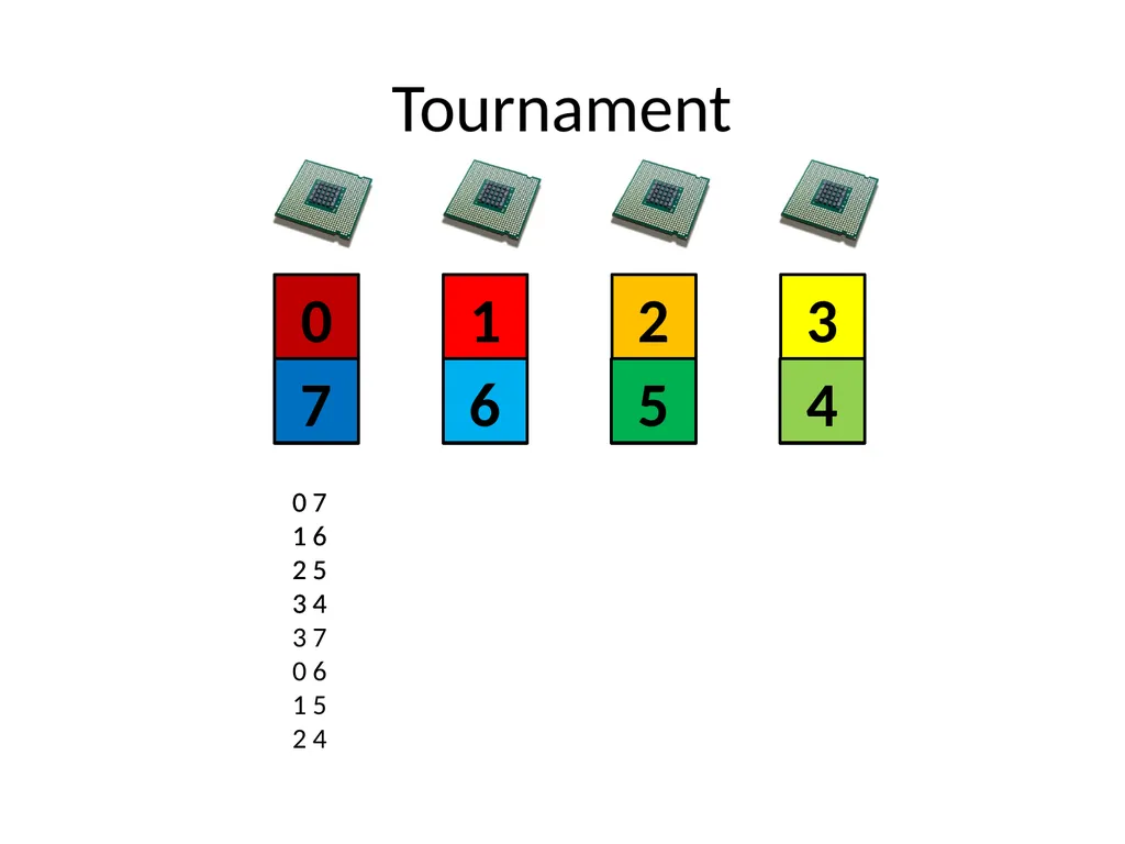
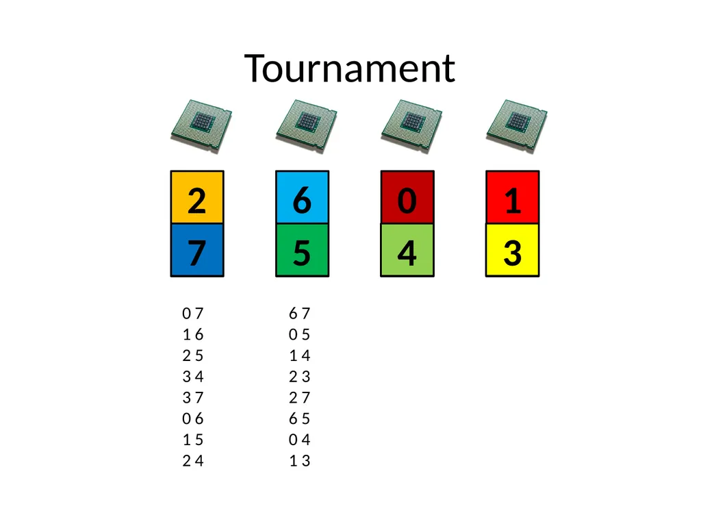
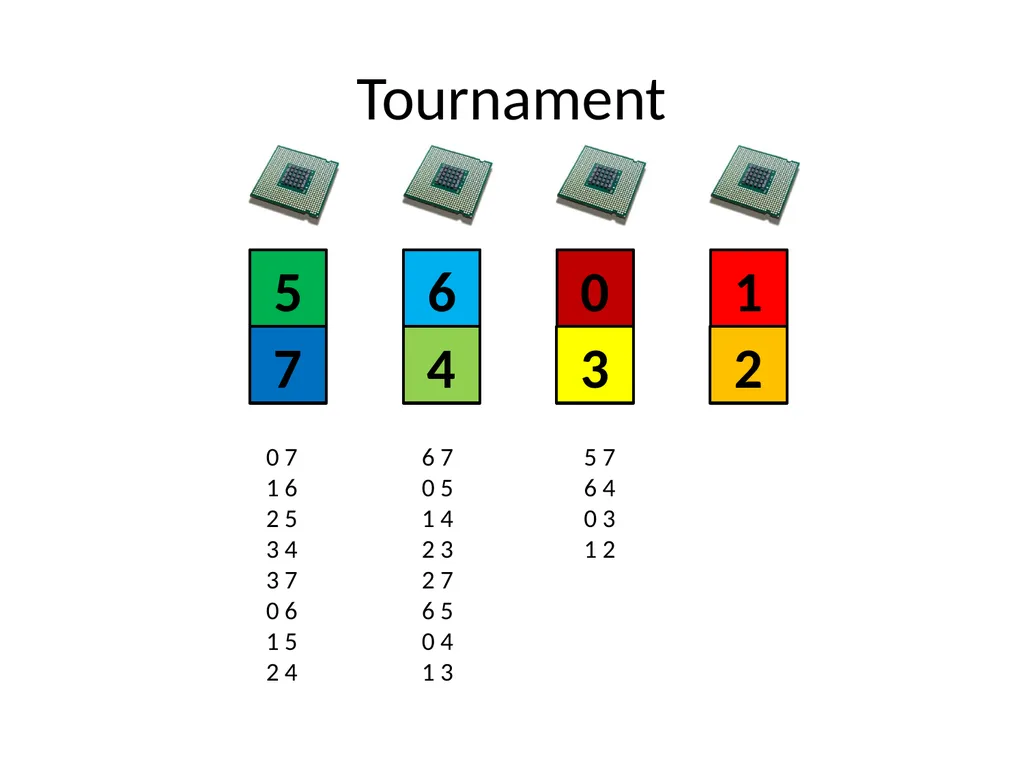
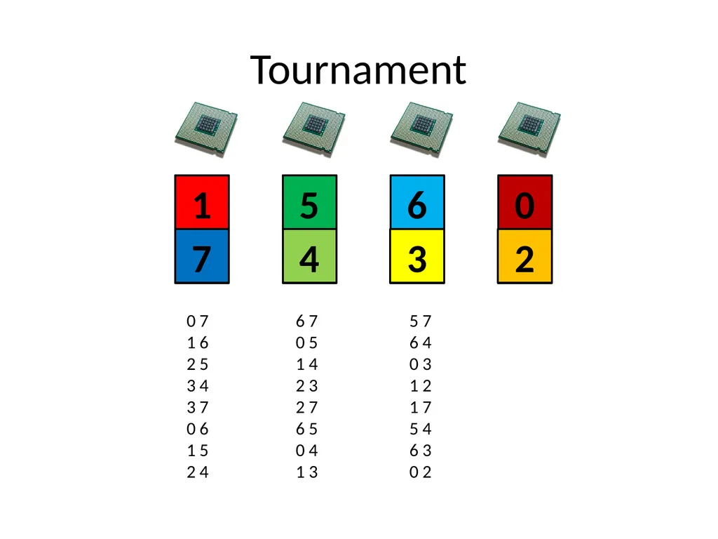
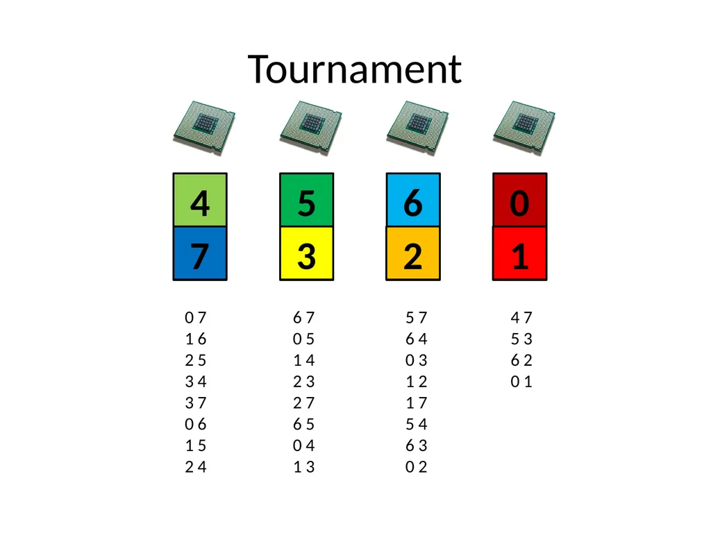
slide103. How can we make sure that each cluster pair is generated exactly once? With minimal communication costs? 
slide104. Tournament 0 1 2 3 7 6 5 4 0 7
1 6
2 5
3 4 0 7
1 6
2 5
3 4
3 7
0 6
1 5
2 4 
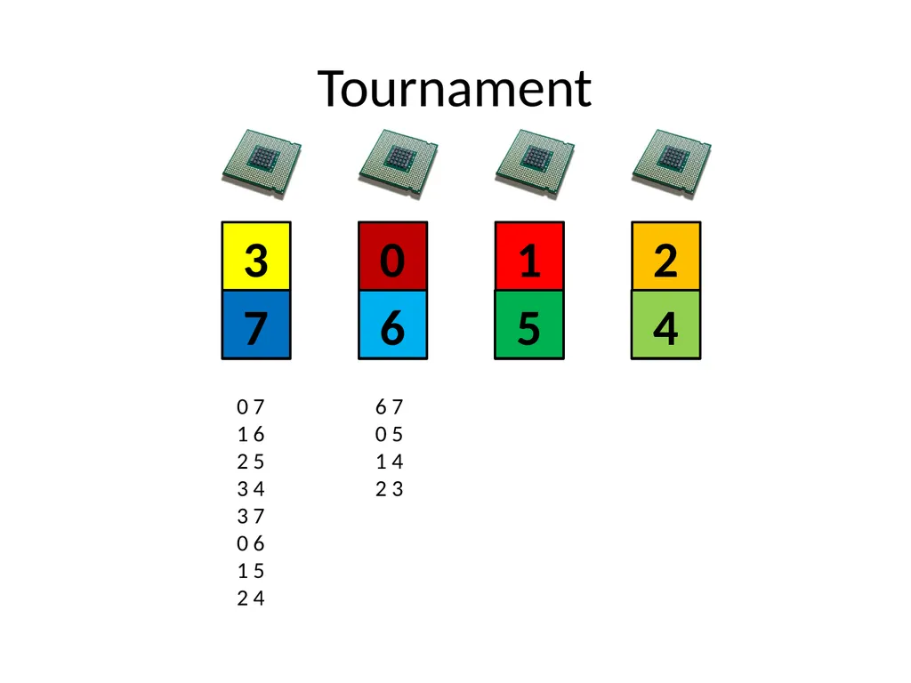
slide105. Tournament 0 1 2 3 7 6 5 4 0 7
1 6
2 5
3 4
3 7
0 6
1 5
2 4 6 7
0 5
1 4
2 3 
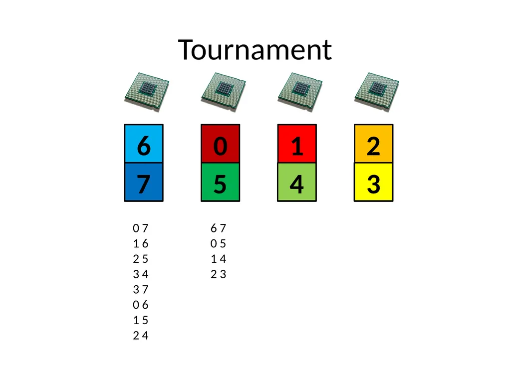
slide106. Tournament 6 0 1 2 7 5 4 3 6 7
0 5
1 4
2 3 0 7
1 6
2 5
3 4
3 7
0 6
1 5
2 4 
slide107. Tournament 6 0 1 2 7 5 4 3 0 7
1 6
2 5
3 4
3 7
0 6
1 5
2 4 6 7
0 5
1 4
2 3
2 7
6 5
0 4
1 3 
slide108. Tournament 5 6 0 1 7 4 3 2 5 7
6 4
0 3
1 2 0 7
1 6
2 5
3 4
3 7
0 6
1 5
2 4 6 7
0 5
1 4
2 3
2 7
6 5
0 4
1 3 
slide109. Tournament 5 6 0 1 7 4 3 2 0 7
1 6
2 5
3 4
3 7
0 6
1 5
2 4 6 7
0 5
1 4
2 3
2 7
6 5
0 4
1 3 5 7
6 4
0 3
1 2
1 7
5 4
6 3
0 2 
slide110. Tournament 4 5 6 0 7 3 2 1 4 7
5 3
6 2
0 1 0 7
1 6
2 5
3 4
3 7
0 6
1 5
2 4 6 7
0 5
1 4
2 3
2 7
6 5
0 4
1 3 5 7
6 4
0 3
1 2
1 7
5 4
6 3
0 2 
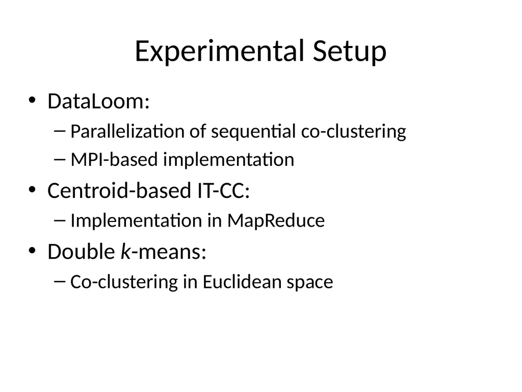
slide111. Experimental Setup DataLoom:
Parallelization of sequential co-clustering
MPI-based implementation
Centroid-based IT-CC:
Implementation in MapReduce
Double k-means:
Co-clustering in Euclidean space 
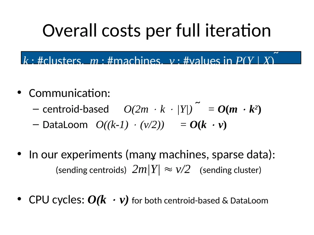
slide112. Overall costs per full iteration k : #clusters, m : #machines, v : #values in P(Y | X)
Communication:
centroid-based O(2m  k  |Y|) = O(m  k2)
DataLoom O((k-1)  (v/2)) = O(k  v)
In our experiments (many machines, sparse data): (sending centroids) 2m|Y|  v/2 (sending cluster)

CPU cycles: O(k  v) for both centroid-based & DataLoom ~ ~ ~ 
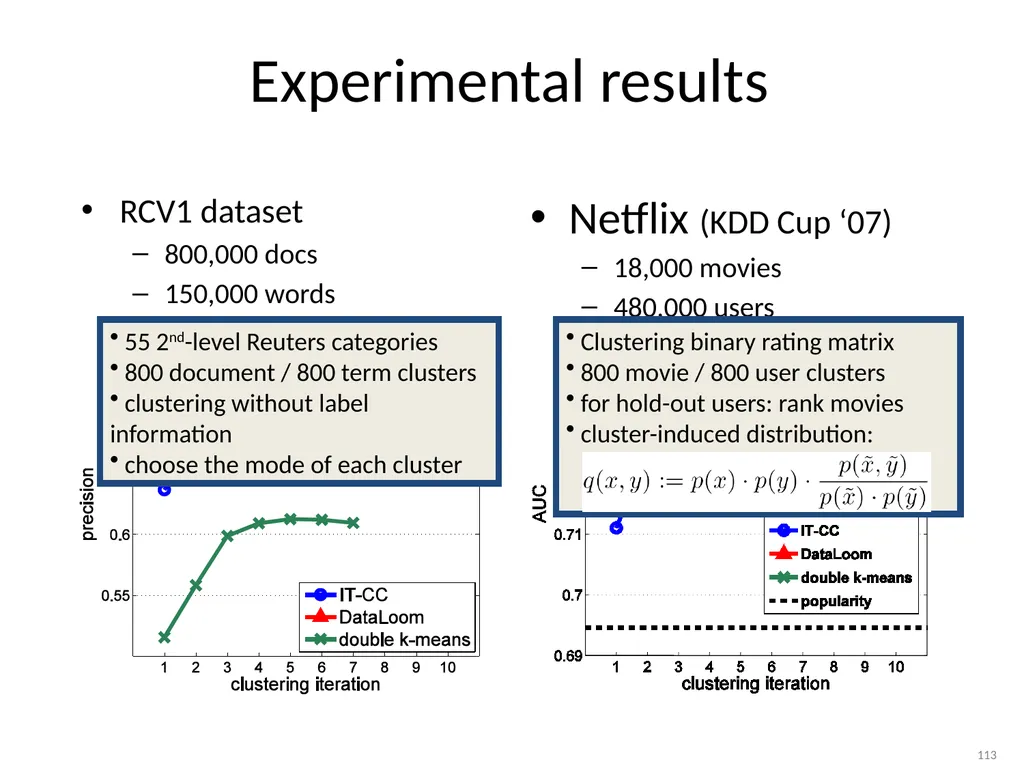
slide113. Experimental results RCV1 dataset
800,000 docs
150,000 words Netflix (KDD Cup ‘07)
18,000 movies
480,000 users 113 55 2nd-level Reuters categories
800 document / 800 term clusters
clustering without label information
choose the mode of each cluster 
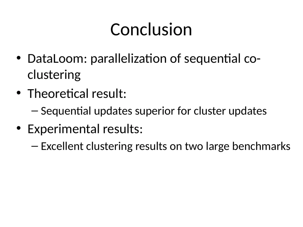
slide114. Conclusion DataLoom: parallelization of sequential co-clustering
Theoretical result:
Sequential updates superior for cluster updates
Experimental results:
Excellent clustering results on two large benchmarks

Scaling Up Machine Learning Parallel and

Related Topics

Share · Embed code

Download Presentation

Presentation Transcript