04
Dictatorial Approach<br>
05
Self-Adaptive Semi-Autonomous �Dictatorial Parent Selection (SASADIPS) Each individual has an evolving mate selection function
First parent selected in a traditional manner
Second parent selected by first parent –the dictator – using its mate selection function<br>
06
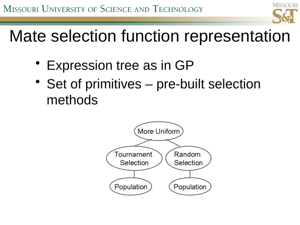
Mate selection function representation Expression tree as in GP
Set of primitives – pre-built selection methods<br>
07
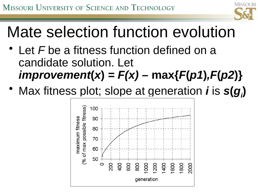
Mate selection function evolution Let F be a fitness function defined on a candidate solution. Let�improvement(x) = F(x) – max{F(p1),F(p2)}
Max fitness plot; slope at generation i is s(gi)<br>
08
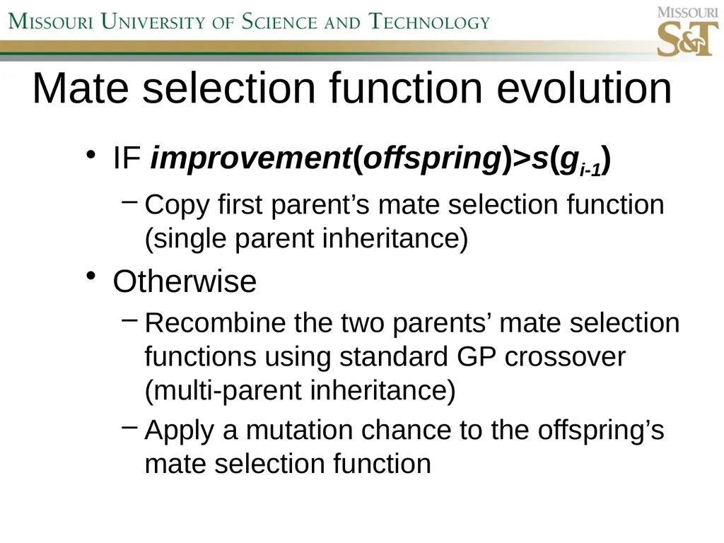
Mate selection function evolution IF improvement(offspring)>s(gi-1)
Copy first parent’s mate selection function (single parent inheritance)
Otherwise
Recombine the two parents’ mate selection functions using standard GP crossover�(multi-parent inheritance)
Apply a mutation chance to the offspring’s mate selection function<br>
09
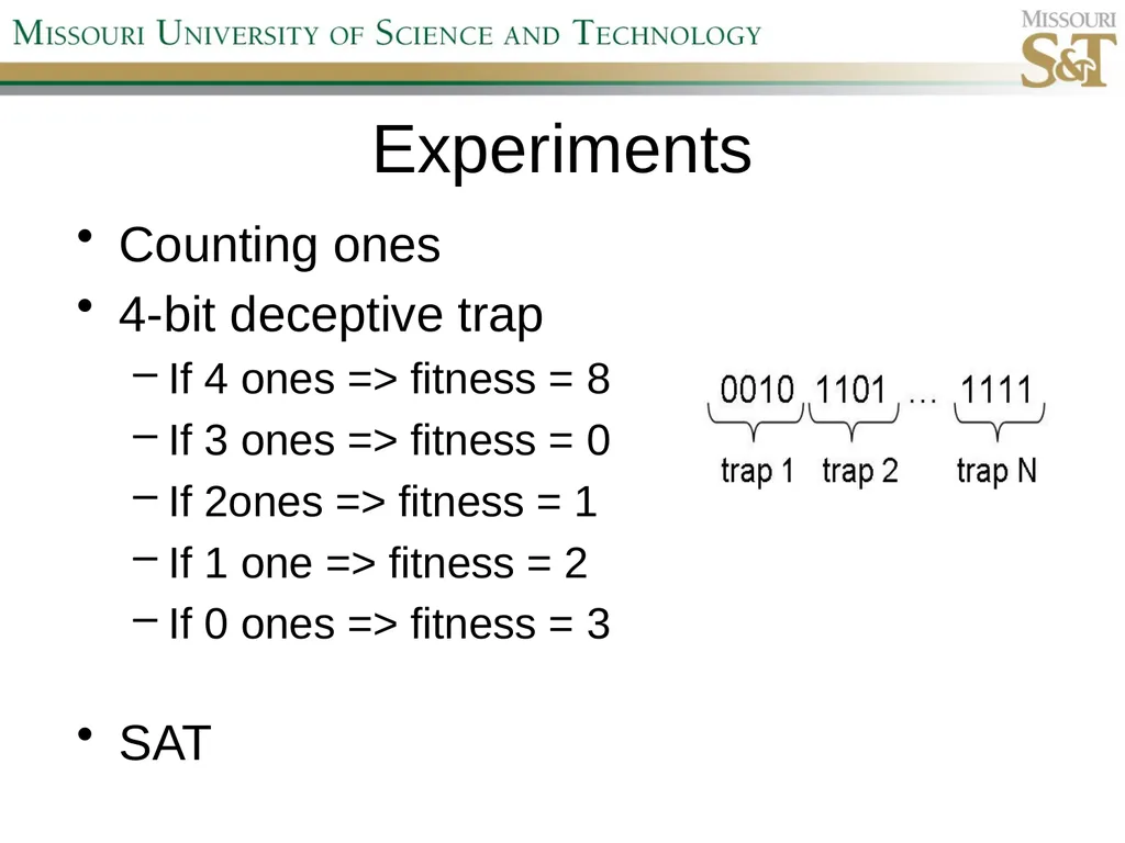
Experiments Counting ones
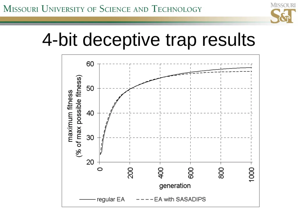
4-bit deceptive trap
If 4 ones => fitness = 8
If 3 ones => fitness = 0
If 2ones => fitness = 1
If 1 one => fitness = 2
If 0 ones => fitness = 3�
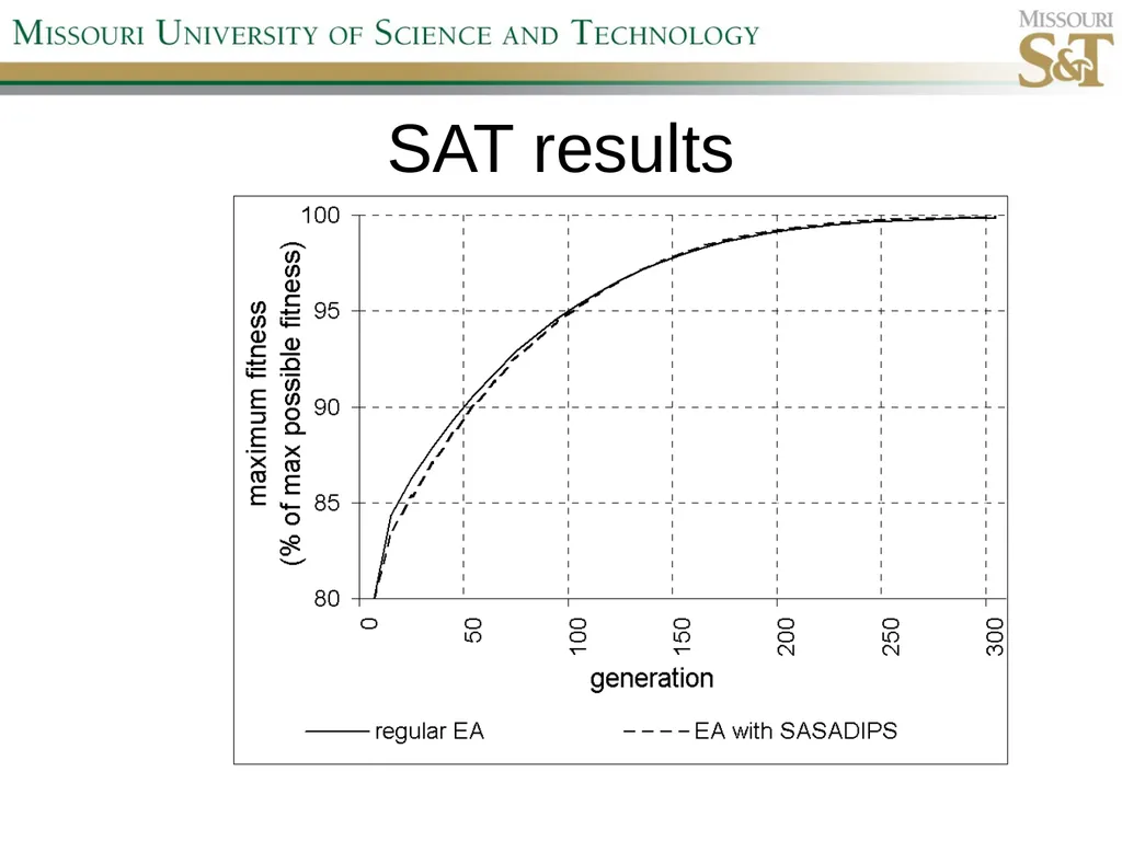
SAT<br>
10
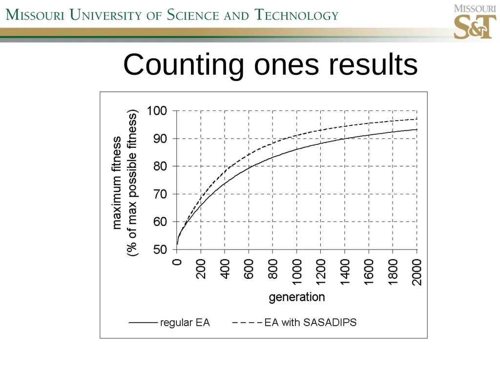
Counting ones results<br>
11
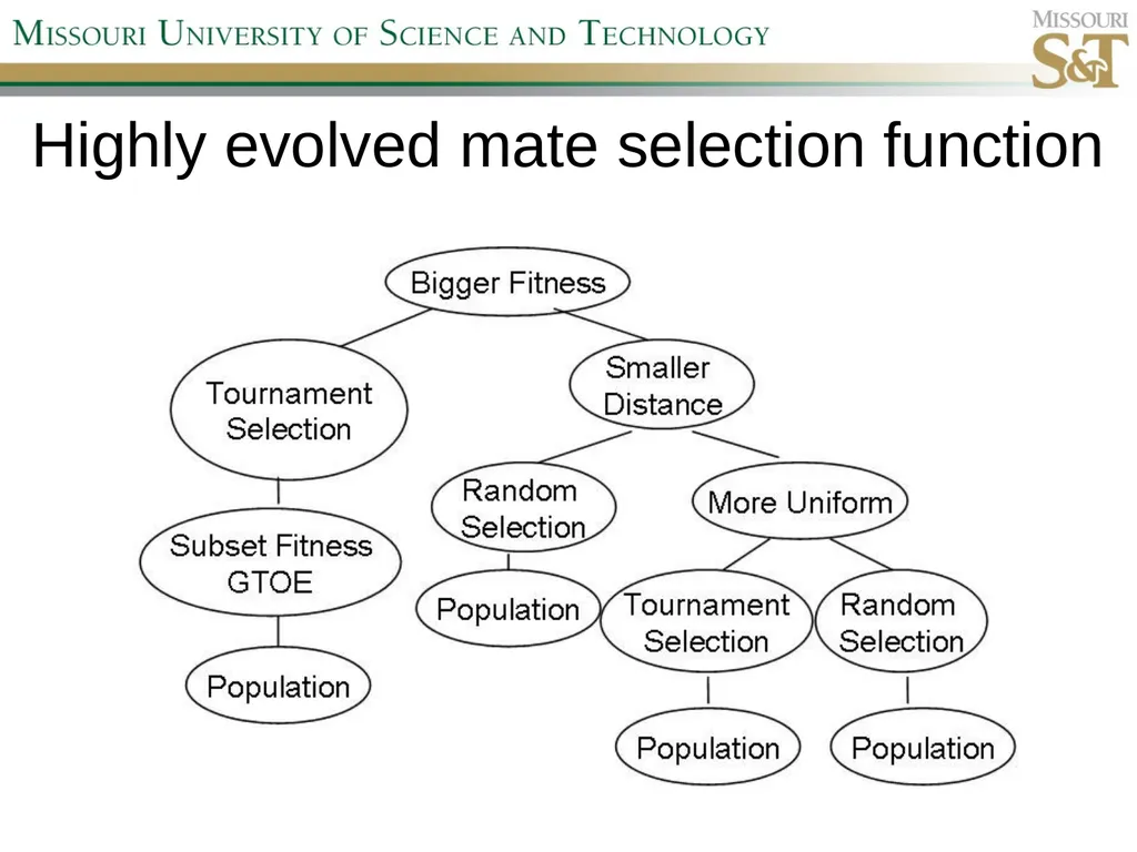
Highly evolved mate selection function<br>
13
4-bit deceptive trap results<br>
14
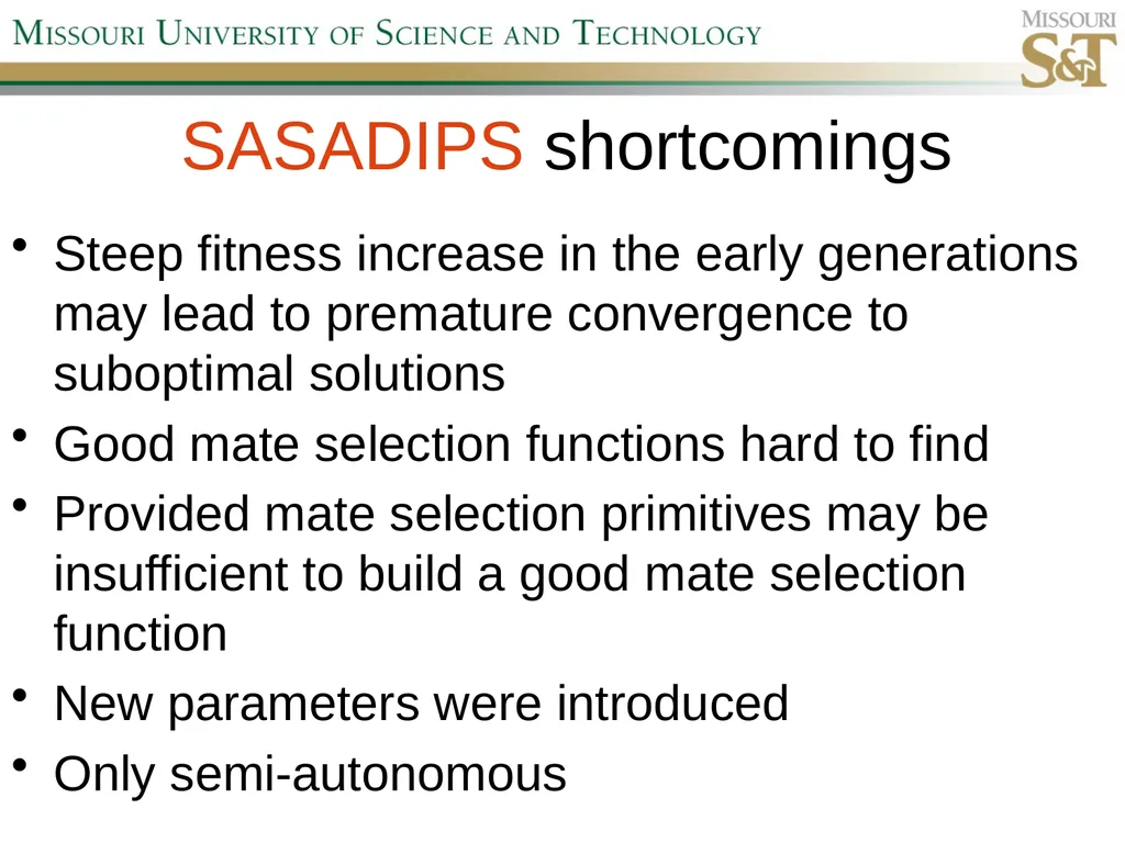
SASADIPS shortcomings Steep fitness increase in the early generations may lead to premature convergence to suboptimal solutions
Good mate selection functions hard to find
Provided mate selection primitives may be insufficient to build a good mate selection function
New parameters were introduced
Only semi-autonomous<br>
15
Greedy Population Sizing�(GPS)<br>
16
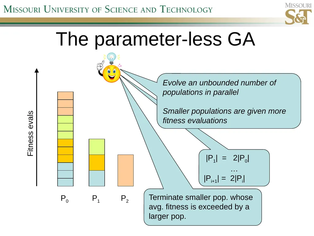
|P1| = 2|P0|
…
|Pi+1| = 2|Pi| The parameter-less GA P0 P1 P2 Evolve an unbounded number of populations in parallel
Smaller populations are given more fitness evaluations Fitness evals Terminate smaller pop. whose avg. fitness is exceeded by a larger pop.<br>
17
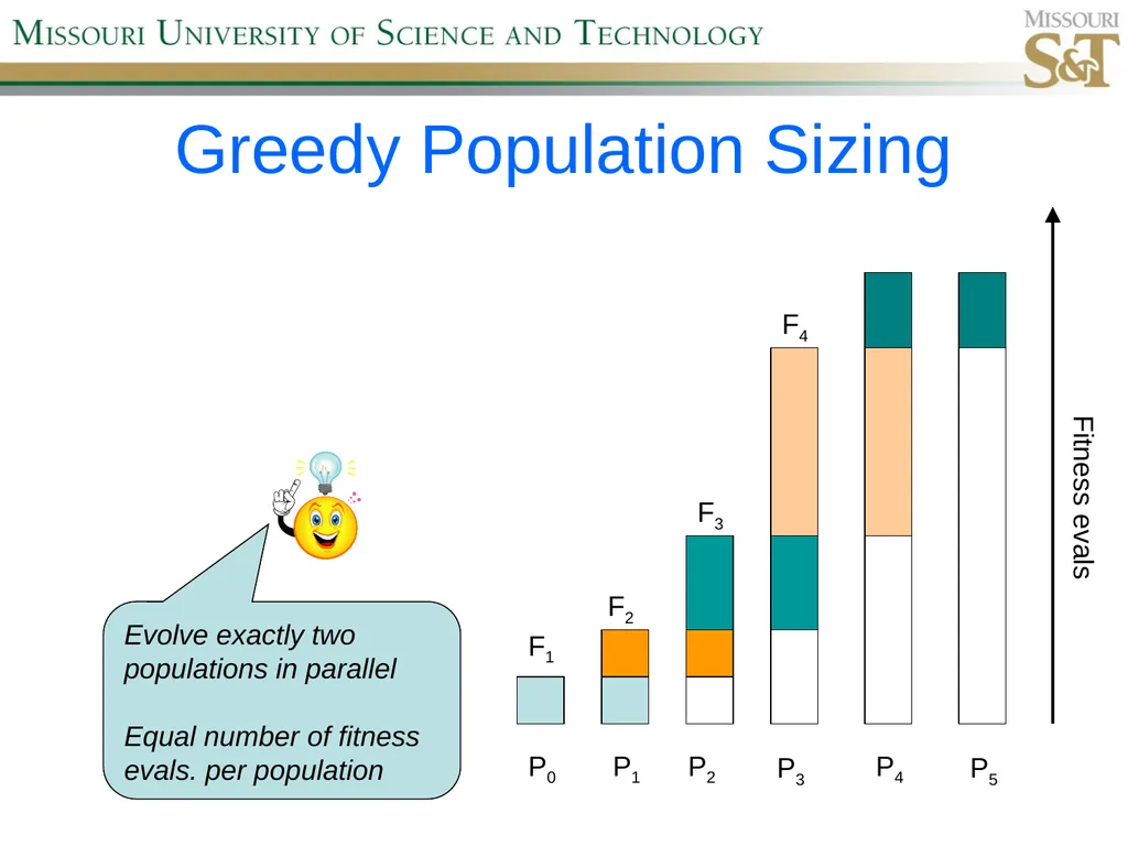
Greedy Population Sizing P0 P1 P2 P3 P4 P5 F1 F2 F3 F4 Evolve exactly two populations in parallel
Equal number of fitness evals. per population Fitness evals<br>
18
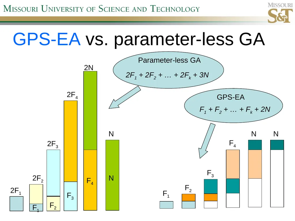
GPS-EA vs. parameter-less GA F1 F2 F3 F4 N N F1 2F1 F2 2F2 F3 2F3 F4 2F4 2F1 + 2F2 + … + 2Fk + 3N N 2N F1 + F2 + … + Fk + 2N N Parameter-less GA GPS-EA<br>
19
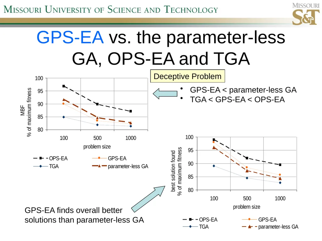
GPS-EA vs. the parameter-less GA, OPS-EA and TGA GPS-EA < parameter-less GA
TGA < GPS-EA < OPS-EA GPS-EA finds overall better
solutions than parameter-less GA Deceptive Problem<br>
20
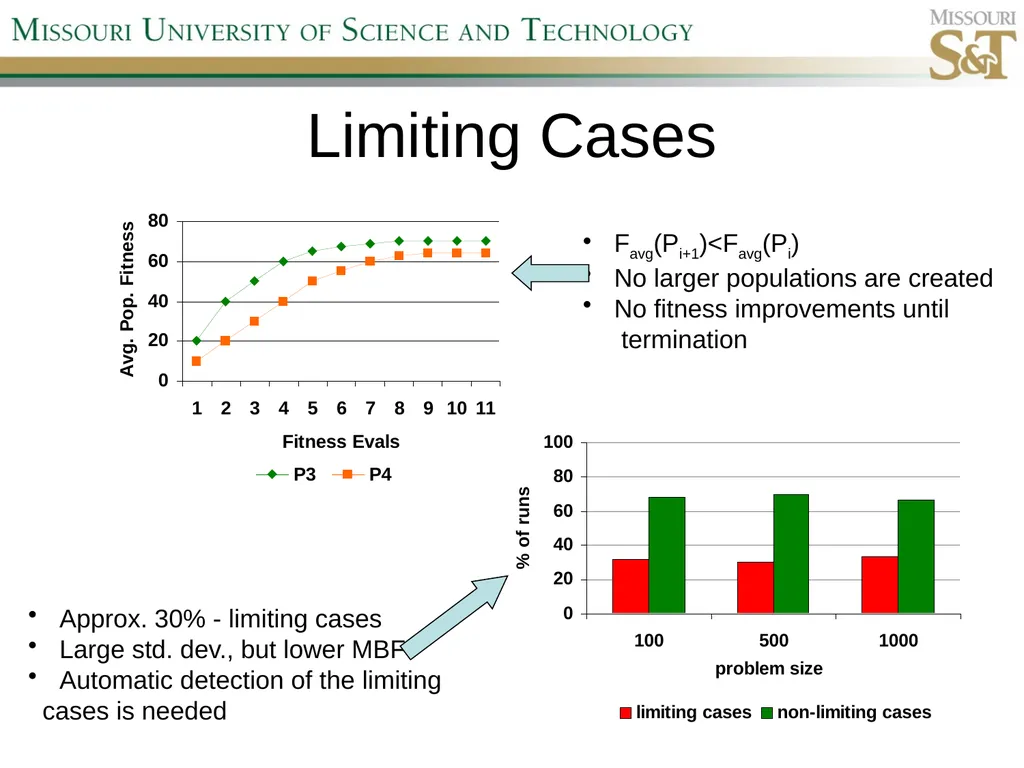
Limiting Cases Favg(Pi+1)<Favg(Pi)
No larger populations are created
No fitness improvements until � termination Approx. 30% - limiting cases
Large std. dev., but lower MBF
Automatic detection of the limiting
cases is needed<br>
21
GPS-EA Summary Advantages
Automated population size control
Finds high quality solutions
Problems
Limiting cases
Restart of evolution each time<br>
22
Estimated Learning Offspring Optimizing�Mate Selection�(ELOOMS)<br>
23
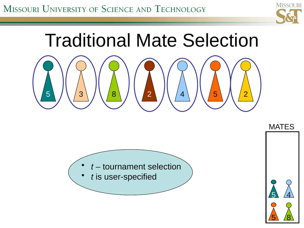
Traditional Mate Selection 2 5 3 8 2 4 5 MATES 5 8 5 4 t – tournament selection
t is user-specified<br>
24
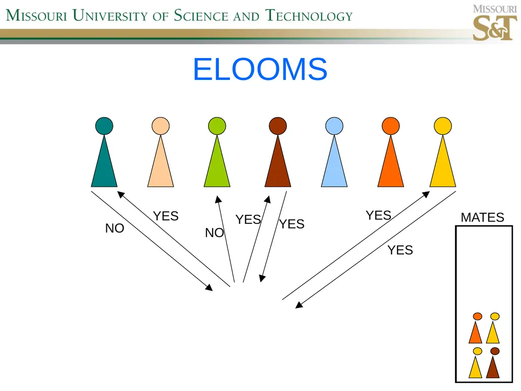
ELOOMS NO YES YES MATES YES NO YES YES<br>
25
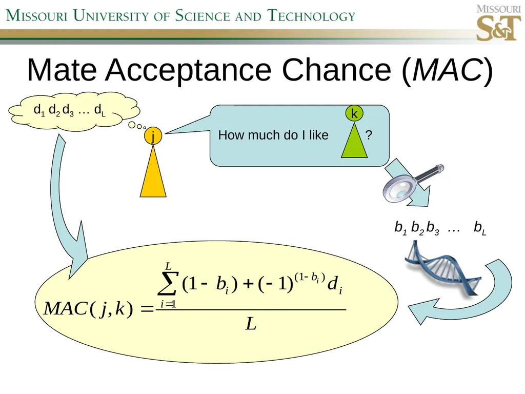
Mate Acceptance Chance (MAC) j How much do I like ? k b1 b2 b3 … bL d1 d2 d3 … dL<br>
26
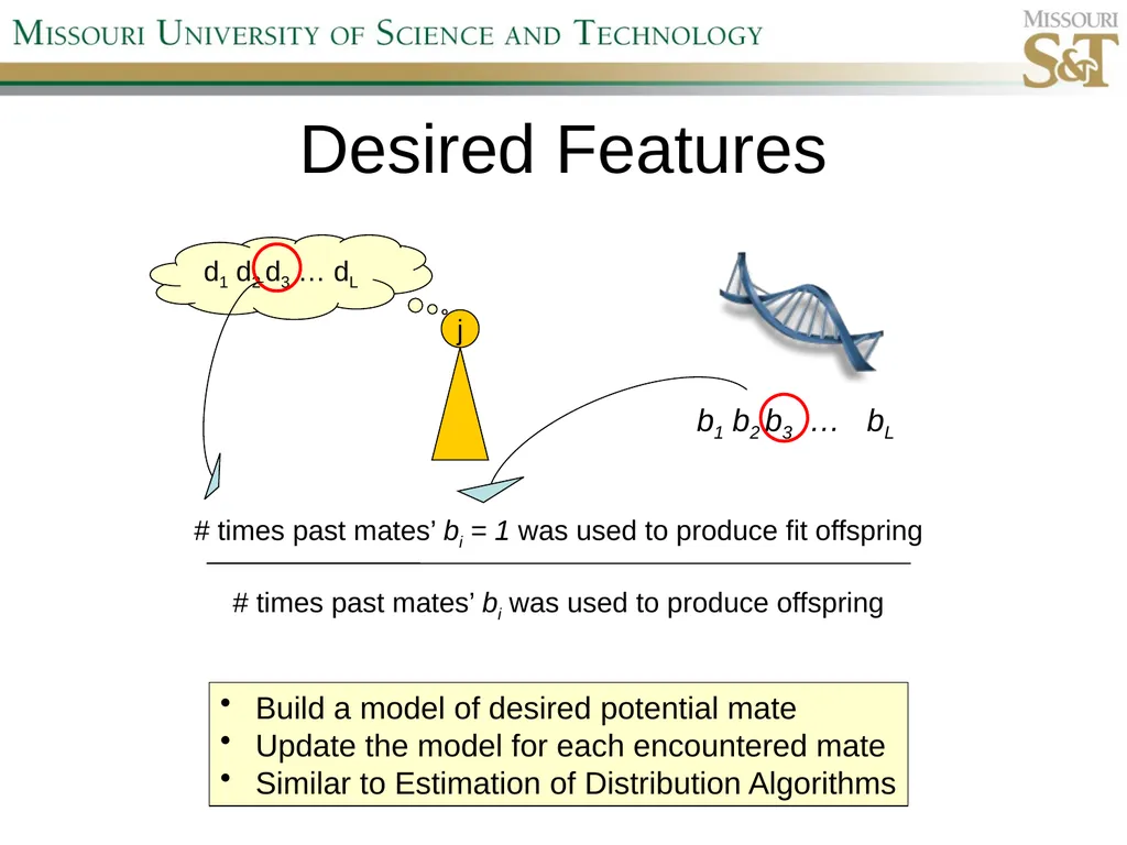
Desired Features j d1 d2 d3 … dL # times past mates’ bi = 1 was used to produce fit offspring
# times past mates’ bi was used to produce offspring b1 b2 b3 … bL Build a model of desired potential mate
Update the model for each encountered mate
Similar to Estimation of Distribution Algorithms<br>
27
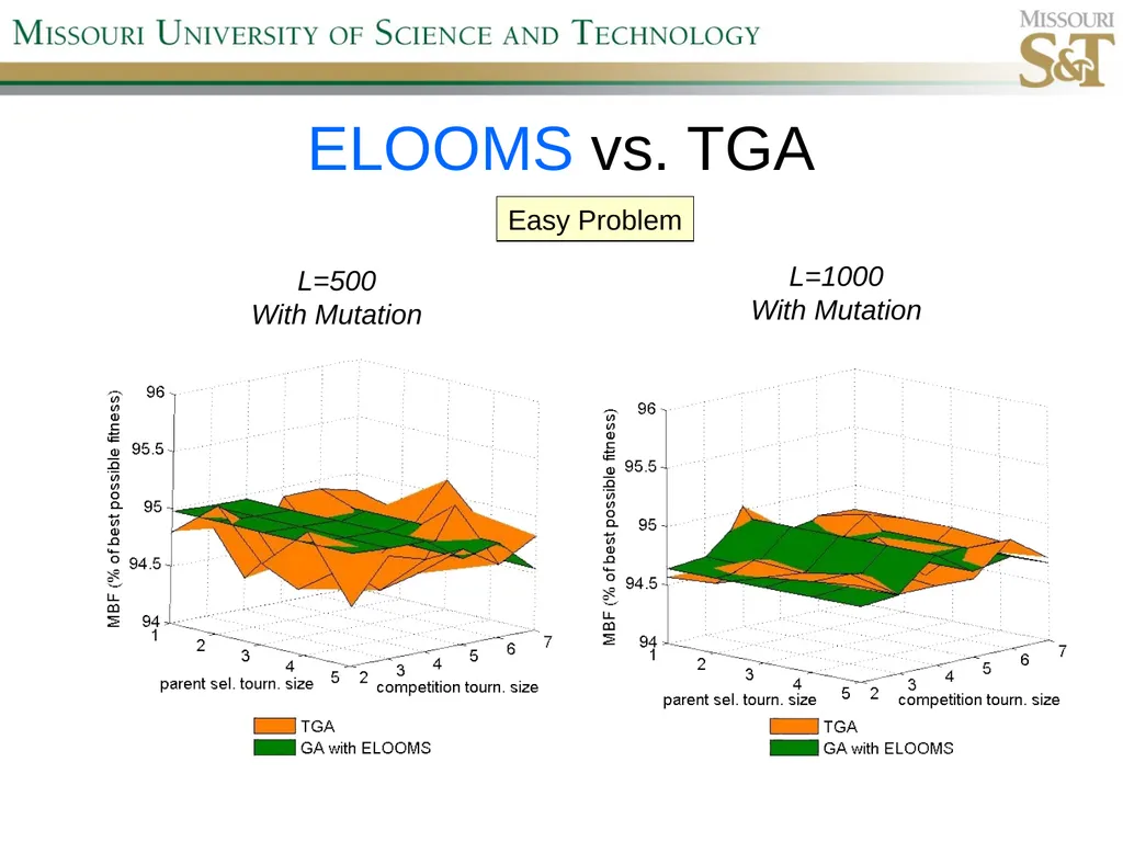
ELOOMS vs. TGA L=500
With Mutation L=1000
With Mutation Easy Problem<br>
28
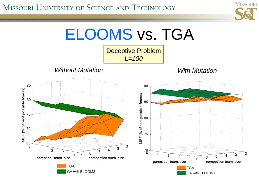
ELOOMS vs. TGA Without Mutation With Mutation Deceptive Problem
L=100<br>
29
Why ELOOMS works on Deceptive Problem More likely to preserve optimal structure
1111 0000 will equally like:
1111 1000
1111 1100
1111 1110
But will dislike individuals not of the form:
1111 xxxx<br>
30
Why ELOOMS does not work as well on Easy Problem High fitness – short distance to optimal
Mating with high fitness individuals – closer to optimal offspring
Fitness – good measure of good mate
ELOOMS – approximate measure of good mate<br>
31
ELOOMS computational overhead L – solution length
μ – population size
T – avg # mates evaluated per individual
Update stage:
6L additions
Mate selection stage:
2L*T* μ additions<br>
32
ELOOMS Summary Advantages
Autonomous mate pairing
Improved performance (some cases)
Natural termination condition
Disadvantages
Relies on competition selection pressure
Computational overhead can be significant<br>
33
GPS-EA + ELOOMS Hybrid<br>
34
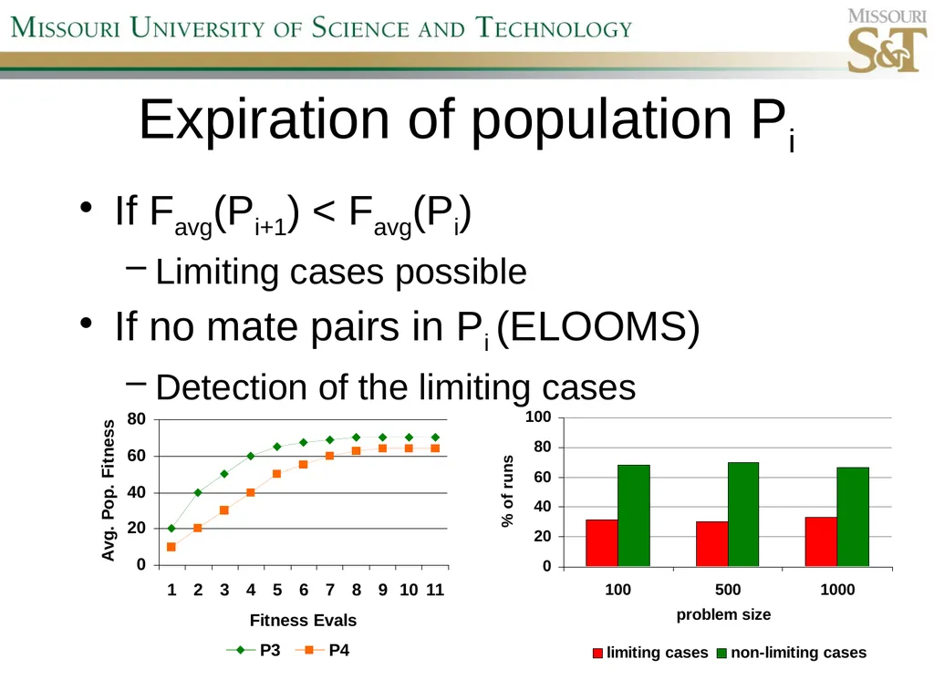
Expiration of population Pi If Favg(Pi+1) < Favg(Pi)
Limiting cases possible
If no mate pairs in Pi (ELOOMS)
Detection of the limiting cases<br>
35
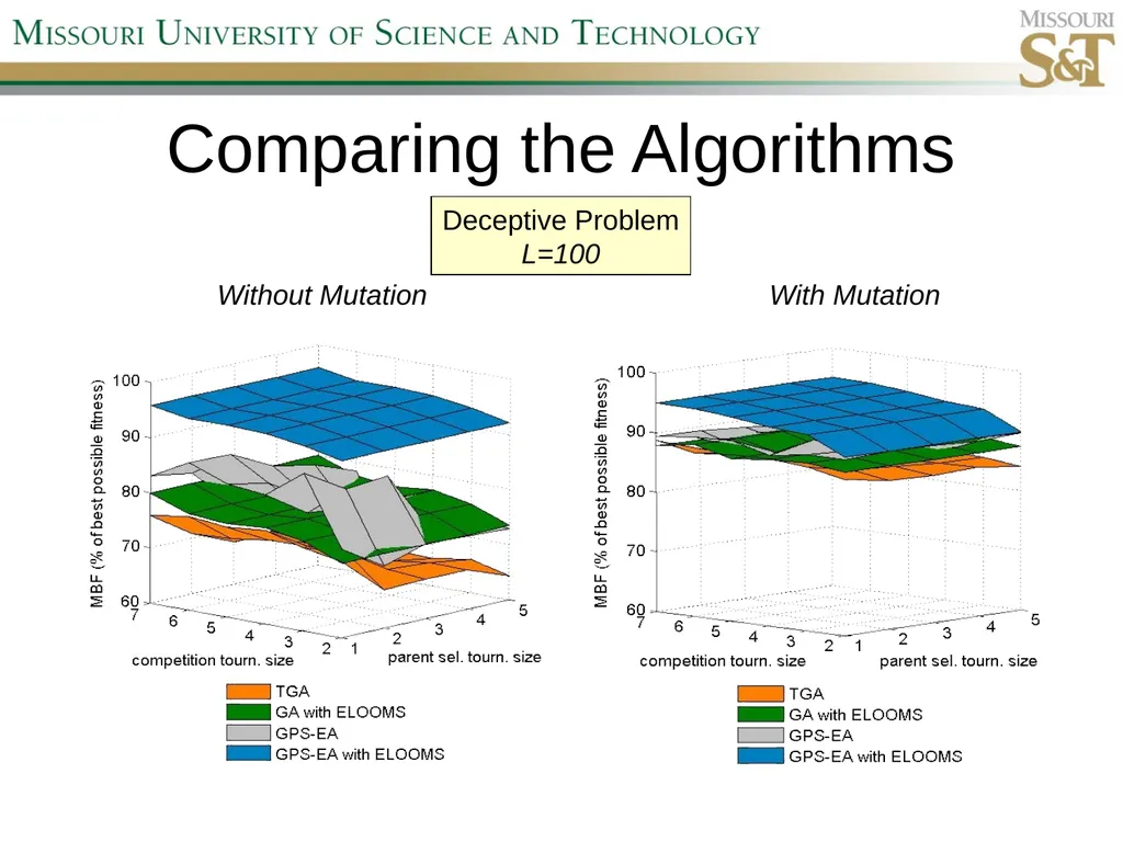
Comparing the Algorithms Without Mutation With Mutation Deceptive Problem
L=100<br>
36
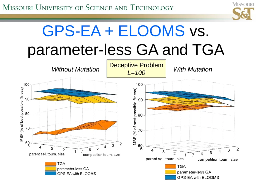
GPS-EA + ELOOMS vs. �parameter-less GA and TGA Without Mutation With Mutation Deceptive Problem
L=100<br>
37
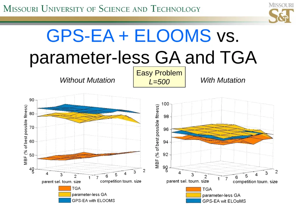
GPS-EA + ELOOMS vs. �parameter-less GA and TGA Without Mutation With Mutation Easy Problem
L=500<br>
38
GPS-EA + ELOOMS Summary Advantages
No population size tuning
No parent selection pressure tuning
No limiting cases
Superior performance on deceptive problem
Disadvantages
Reduced performance on easy problem
Relies on competition selection pressure<br>