
Sorting Algorithms Properties Insertion Sort
Description: Sorting Algorithms Properties Insertion Sort Binary Search CSE 3318 Algorithms and Data Structures Alexandra Stefan University of Texas at Arlington 1 1162025 Summary Properties of sorting algorithms Sorting algorithms Insertion sort
Related Topics
Download Presentation
"Sorting Algorithms Properties Insertion Sort" is the property of its rightful owner. Permission is granted to download and print the materials on this website for personal, non-commercial use only, and to display it on your personal computer provided you do not modify the materials and that you retain all copyright notices contained in the materials. By downloading content from our website, you accept the terms of this agreement.
Presentation Transcript
slide1. Sorting Algorithms Properties
Insertion Sort
Binary Search CSE 3318 – Algorithms and Data Structures
Alexandra Stefan
University of Texas at Arlington 1 1/16/2025<br>
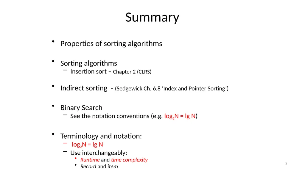
slide2. Summary Properties of sorting algorithms
Sorting algorithms
Insertion sort – Chapter 2 (CLRS)
Indirect sorting - (Sedgewick Ch. 6.8 ‘Index and Pointer Sorting’)
Binary Search
See the notation conventions (e.g. log2N = lg N)
Terminology and notation:
log2N = lg N
Use interchangeably:
Runtime and time complexity
Record and item 2<br>
slide3. Sorting 3<br>
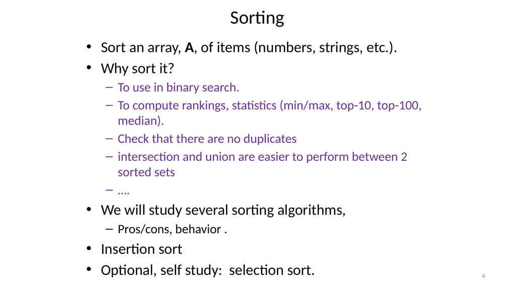
slide4. Sorting Sort an array, A, of items (numbers, strings, etc.).
Why sort it?
To use in binary search.
To compute rankings, statistics (min/max, top-10, top-100, median).
Check that there are no duplicates
intersection and union are easier to perform between 2 sorted sets
….
We will study several sorting algorithms,
Pros/cons, behavior .
Insertion sort
Optional, self study: selection sort. 4<br>
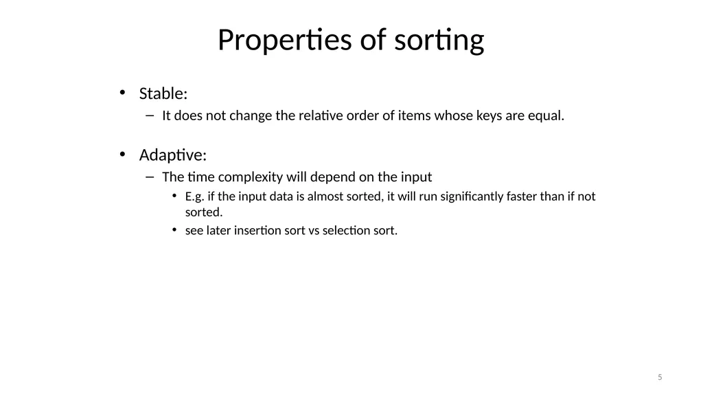
slide5. Properties of sorting Stable:
It does not change the relative order of items whose keys are equal.
Adaptive:
The time complexity will depend on the input
E.g. if the input data is almost sorted, it will run significantly faster than if not sorted.
see later insertion sort vs selection sort. 5<br>
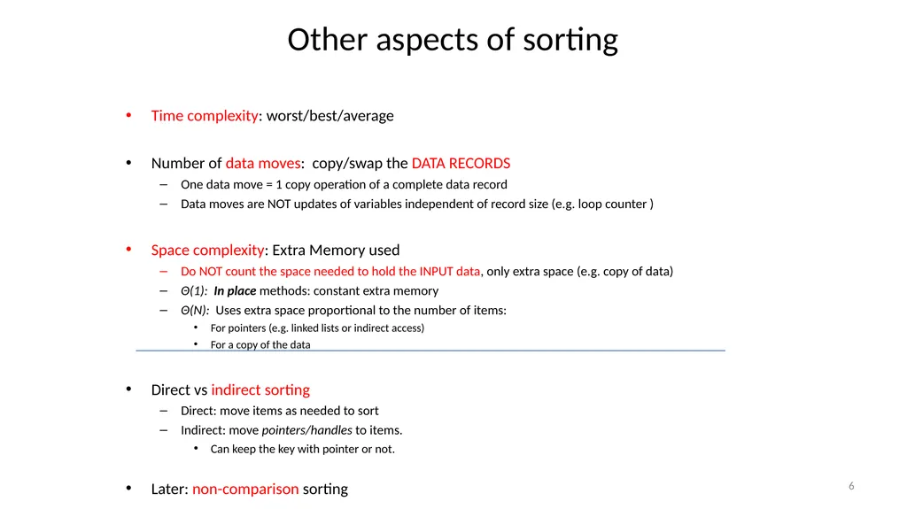
slide6. Other aspects of sorting Time complexity: worst/best/average
Number of data moves: copy/swap the DATA RECORDS
One data move = 1 copy operation of a complete data record
Data moves are NOT updates of variables independent of record size (e.g. loop counter )
Space complexity: Extra Memory used
Do NOT count the space needed to hold the INPUT data, only extra space (e.g. copy of data)
Θ(1): In place methods: constant extra memory
Θ(N): Uses extra space proportional to the number of items:
For pointers (e.g. linked lists or indirect access)
For a copy of the data
Direct vs indirect sorting
Direct: move items as needed to sort
Indirect: move pointers/handles to items.
Can keep the key with pointer or not.
Later: non-comparison sorting 6<br>
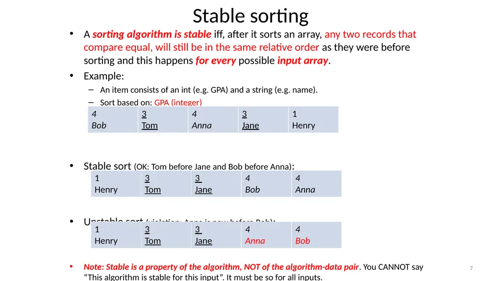
slide7. Stable sorting A sorting algorithm is stable iff, after it sorts an array, any two records that compare equal, will still be in the same relative order as they were before sorting and this happens for every possible input array.
Example:
An item consists of an int (e.g. GPA) and a string (e.g. name).
Sort based on: GPA (integer)
Stable sort (OK: Tom before Jane and Bob before Anna):
Unstable sort (violation: Anna is now before Bob):
Note: Stable is a property of the algorithm, NOT of the algorithm-data pair. You CANNOT say “This algorithm is stable for this input”. It must be so for all inputs. 7<br>
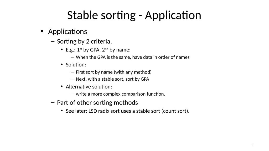
slide8. Stable sorting - Application Applications
Sorting by 2 criteria,
E.g.: 1st by GPA, 2nd by name:
When the GPA is the same, have data in order of names
Solution:
First sort by name (with any method)
Next, with a stable sort, sort by GPA
Alternative solution:
write a more complex comparison function.
Part of other sorting methods
See later: LSD radix sort uses a stable sort (count sort). 8<br>
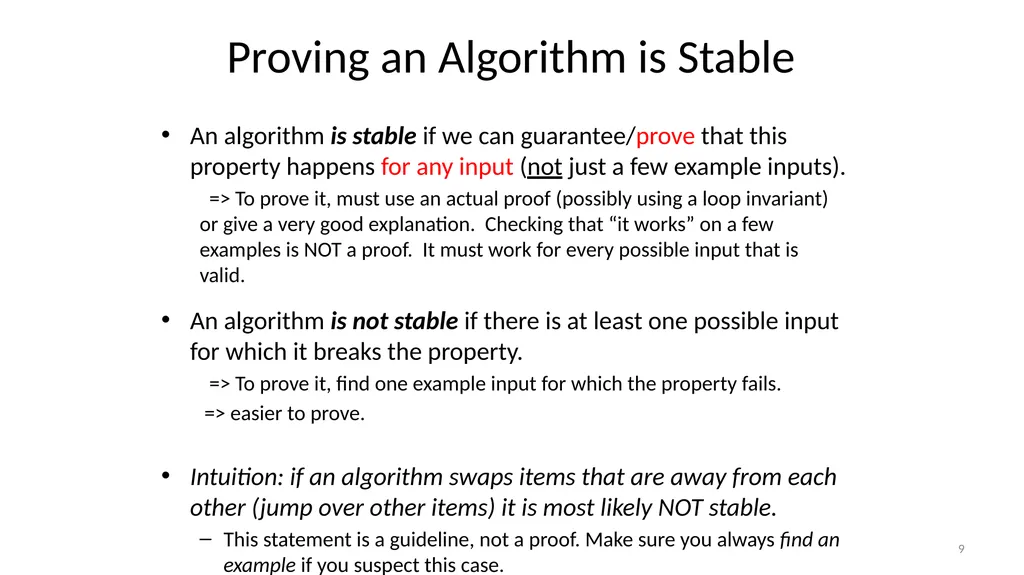
slide9. Proving an Algorithm is Stable An algorithm is stable if we can guarantee/prove that this property happens for any input (not just a few example inputs).
=> To prove it, must use an actual proof (possibly using a loop invariant) or give a very good explanation. Checking that “it works” on a few examples is NOT a proof. It must work for every possible input that is valid.
An algorithm is not stable if there is at least one possible input for which it breaks the property.
=> To prove it, find one example input for which the property fails.
=> easier to prove.
Intuition: if an algorithm swaps items that are away from each other (jump over other items) it is most likely NOT stable.
This statement is a guideline, not a proof. Make sure you always find an example if you suspect this case. 9<br>
slide10. Insertion sort 10<br>
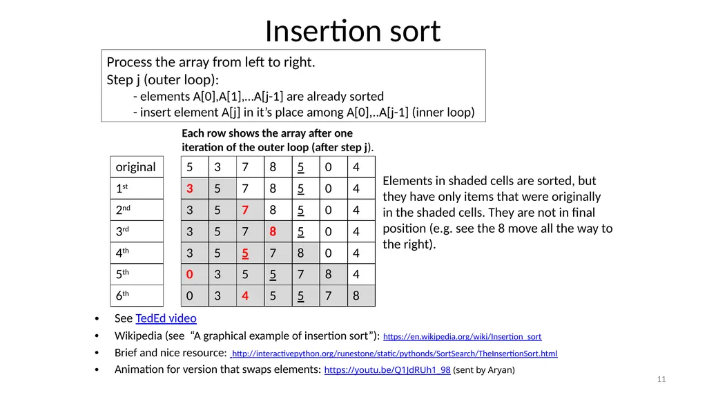
slide11. Insertion sort 11 Each row shows the array after one iteration of the outer loop (after step j). Process the array from left to right.
Step j (outer loop):
- elements A[0],A[1],…A[j-1] are already sorted
- insert element A[j] in it’s place among A[0],..A[j-1] (inner loop) Elements in shaded cells are sorted, but they have only items that were originally in the shaded cells. They are not in final position (e.g. see the 8 move all the way to the right). See TedEd video
Wikipedia (see “A graphical example of insertion sort”): https://en.wikipedia.org/wiki/Insertion_sort
Brief and nice resource: http://interactivepython.org/runestone/static/pythonds/SortSearch/TheInsertionSort.html
Animation for version that swaps elements: https://youtu.be/Q1JdRUh1_98 (sent by Aryan)<br>
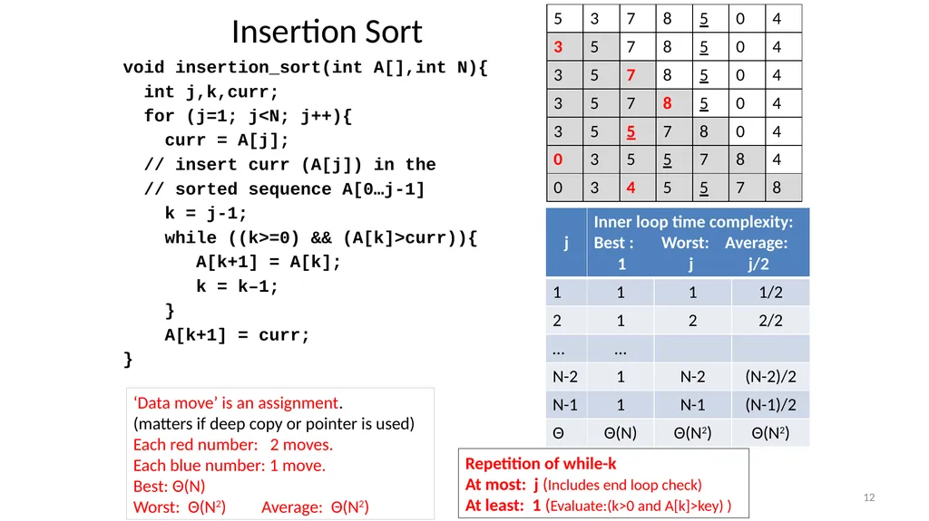
slide12. Insertion Sort 12 Repetition of while-k
At most: j (Includes end loop check)
At least: 1 (Evaluate:(k>0 and A[k]>key) ) void insertion_sort(int A[],int N){
int j,k,curr;
for (j=1; j<N; j++){
curr = A[j];
// insert curr (A[j]) in the
// sorted sequence A[0…j-1]
k = j-1;
while ((k>=0) && (A[k]>curr)){
A[k+1] = A[k];
k = k–1;
}
A[k+1] = curr;
} ‘Data move’ is an assignment.
(matters if deep copy or pointer is used)
Each red number: 2 moves.
Each blue number: 1 move.
Best: Θ(N)
Worst: Θ(N2) Average: Θ(N2)<br>
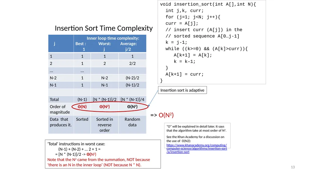
slide13. Insertion Sort Time Complexity 13 ‘Total’ instructions in worst case:
(N-1) + (N-2) + … 2 + 1 =
= [N * (N-1)]/2 -> Θ(N2)
Note that the N2 came from the summation, NOT because ‘there is an N in the inner loop’ (NOT because N * N). => O(N2) “O” will be explained in detail later. It says that the algorithm take at most order of N2.
See the Khan Academy for a discussion on the use of O(N2):
https://www.khanacademy.org/computing/computer-science/algorithms/insertion-sort/a/insertion-sort Insertion sort is adaptive void insertion_sort(int A[],int N){
int j,k, curr;
for (j=1; j<N; j++){
curr = A[j];
// insert curr (A[j]) in the
// sorted sequence A[0…j-1]
k = j-1;
while ((k>=0) && (A[k]>curr)){
A[k+1] = A[k];
k = k–1;
}
A[k+1] = curr;
}<br>
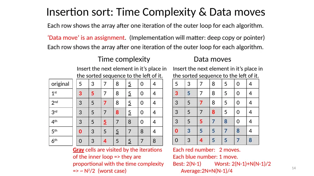
slide14. Insertion sort: Time Complexity & Data moves 14 Time complexity Each row shows the array after one iteration of the outer loop for each algorithm.
‘Data move’ is an assignment. (Implementation will matter: deep copy or pointer)
Each row shows the array after one iteration of the outer loop for each algorithm. Insert the next element in it’s place in the sorted sequence to the left of it. Gray cells are visited by the iterations of the inner loop => they are proportional with the time complexity => ~ N2/2 (worst case) Data moves Insert the next element in it’s place in the sorted sequence to the left of it. Each red number: 2 moves.
Each blue number: 1 move.
Best: 2(N-1) Worst: 2(N-1)+N(N-1)/2 Average:2N+N(N-1)/4<br>
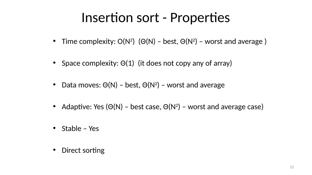
slide15. Insertion sort - Properties Time complexity: O(N2) (Θ(N) – best, Θ(N2) – worst and average )
Space complexity: Θ(1) (it does not copy any of array)
Data moves: Θ(N) – best, Θ(N2) – worst and average
Adaptive: Yes (Θ(N) – best case, Θ(N2) – worst and average case)
Stable – Yes
Direct sorting 15<br>
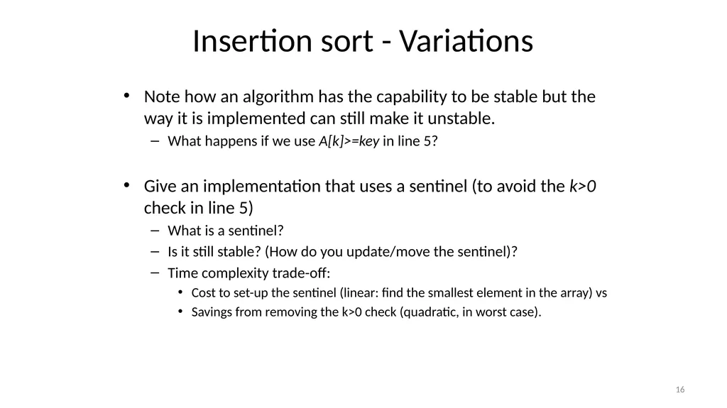
slide16. Insertion sort - Variations Note how an algorithm has the capability to be stable but the way it is implemented can still make it unstable.
What happens if we use A[k]>=key in line 5?
Give an implementation that uses a sentinel (to avoid the k>0 check in line 5)
What is a sentinel?
Is it still stable? (How do you update/move the sentinel)?
Time complexity trade-off:
Cost to set-up the sentinel (linear: find the smallest element in the array) vs
Savings from removing the k>0 check (quadratic, in worst case). 16<br>
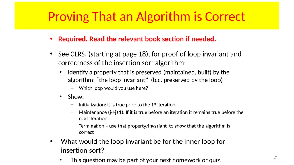
slide17. Proving That an Algorithm is Correct Required. Read the relevant book section if needed.
See CLRS, (starting at page 18), for proof of loop invariant and correctness of the insertion sort algorithm:
Identify a property that is preserved (maintained, built) by the algorithm: “the loop invariant” (b.c. preserved by the loop)
Which loop would you use here?
Show:
Initialization: it is true prior to the 1st iteration
Maintenance (j->j+1): If it is true before an iteration it remains true before the next iteration
Termination – use that property/invariant to show that the algorithm is correct
What would the loop invariant be for the inner loop for insertion sort?
This question may be part of your next homework or quiz. 17<br>
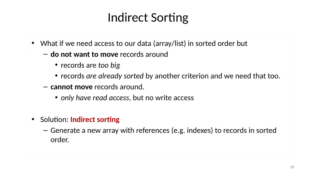
slide18. Indirect Sorting What if we need access to our data (array/list) in sorted order but
do not want to move records around
records are too big
records are already sorted by another criterion and we need that too.
cannot move records around.
only have read access, but no write access
Solution: Indirect sorting
Generate a new array with references (e.g. indexes) to records in sorted order. 18<br>
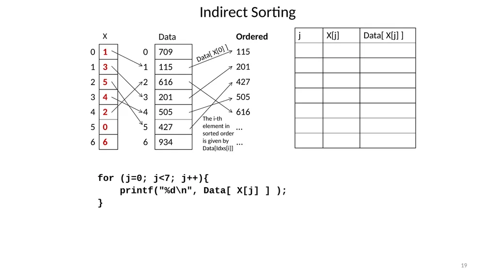
slide19. Indirect Sorting 19 Data[ X[0] ] The i-th element in sorted order is given by Data[Idxs[i]] for (j=0; j<7; j++){
printf("%d\n", Data[ X[j] ] );
}<br>
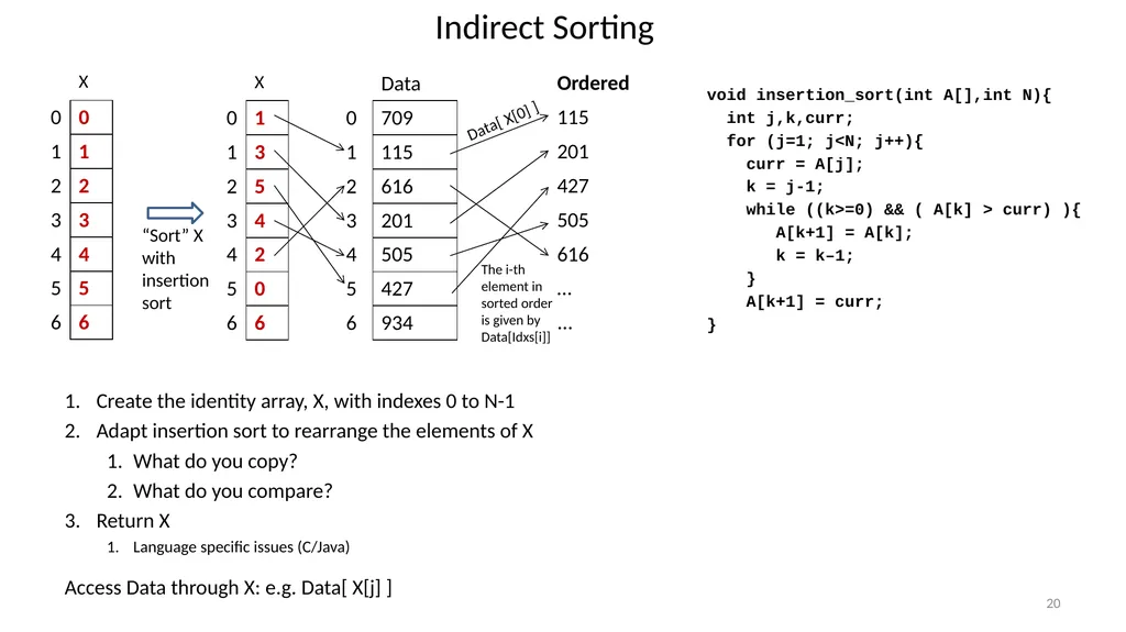
slide20. Indirect Sorting 20 Data[ X[0] ] The i-th element in sorted order is given by Data[Idxs[i]] “Sort” X with insertion sort Create the identity array, X, with indexes 0 to N-1
Adapt insertion sort to rearrange the elements of X
What do you copy?
What do you compare?
Return X
Language specific issues (C/Java)
Access Data through X: e.g. Data[ X[j] ] void insertion_sort(int A[],int N){
int j,k,curr;
for (j=1; j<N; j++){
curr = A[j];
k = j-1;
while ((k>=0) && ( A[k] > curr) ){
A[k+1] = A[k];
k = k–1;
}
A[k+1] = curr;
}<br>
slide21. Indirect Sorting Food for thought:
Example of references:
indexes
memory addresses
offsets in a file
Can we indirect sort a linked list? 21<br>
slide22. Binary Search and Indirect Sorting 22<br>
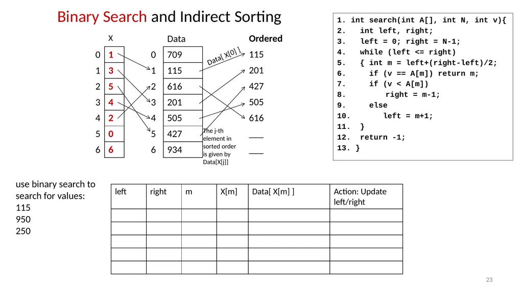
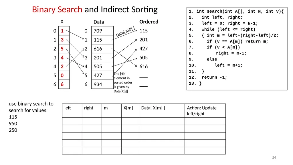
slide23. Binary Search and Indirect Sorting 23 Data[ X[0] ] The j-th element in sorted order is given by Data[X[j]] 1. int search(int A[], int N, int v){
2. int left, right;
3. left = 0; right = N-1;
4. while (left <= right)
5. { int m = left+(right-left)/2;
6. if (v == A[m]) return m;
7. if (v < A[m])
8. right = m-1;
9. else
10. left = m+1;
11. }
12. return -1;
13. } use binary search to
search for values:
115
950
250<br>
slide24. Binary Search and Indirect Sorting 24 Data[ X[0] ] The j-th element in sorted order is given by Data[X[j]] 1. int search(int A[], int N, int v){
2. int left, right;
3. left = 0; right = N-1;
4. while (left <= right)
5. { int m = left+(right-left)/2;
6. if (v == A[m]) return m;
7. if (v < A[m])
8. right = m-1;
9. else
10. left = m+1;
11. }
12. return -1;
13. } use binary search to
search for values:
115
950
250<br>
slide25. Binary Search 25<br>
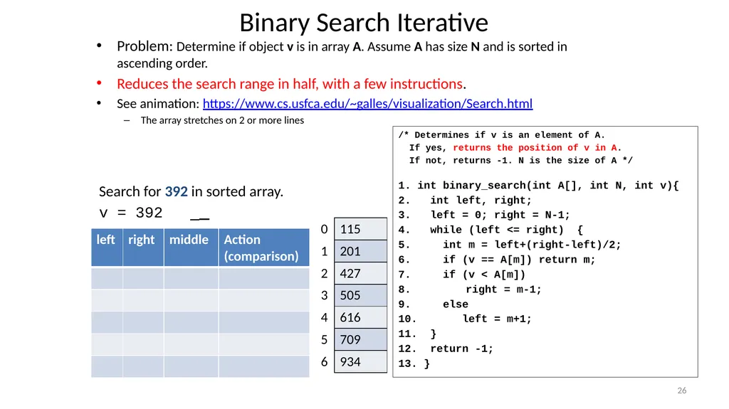
slide26. Binary Search Iterative Search for 392 in sorted array.
v = 392 26 /* Determines if v is an element of A.
If yes, returns the position of v in A.
If not, returns -1. N is the size of A */
1. int binary_search(int A[], int N, int v){
2. int left, right;
3. left = 0; right = N-1;
4. while (left <= right) {
5. int m = left+(right-left)/2;
6. if (v == A[m]) return m;
7. if (v < A[m])
8. right = m-1;
9. else
10. left = m+1;
11. }
12. return -1;
13. } Problem: Determine if object v is in array A. Assume A has size N and is sorted in ascending order.
Reduces the search range in half, with a few instructions.
See animation: https://www.cs.usfca.edu/~galles/visualization/Search.html
The array stretches on 2 or more lines<br>
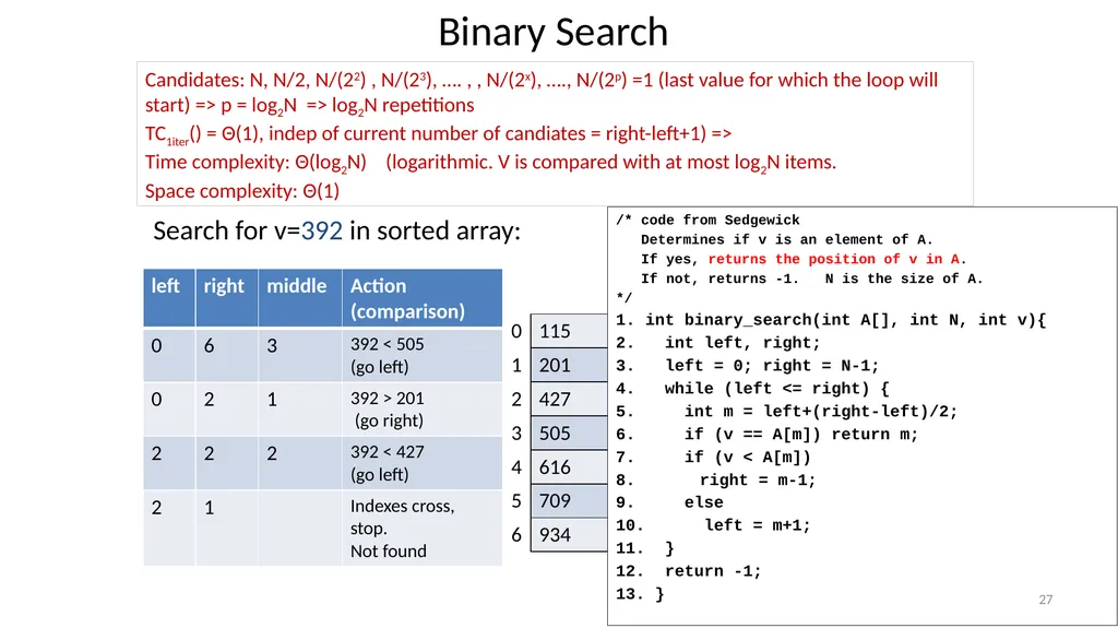
slide27. Binary Search Search for v=392 in sorted array: 27 /* code from Sedgewick
Determines if v is an element of A.
If yes, returns the position of v in A.
If not, returns -1. N is the size of A.
*/
1. int binary_search(int A[], int N, int v){
2. int left, right;
3. left = 0; right = N-1;
4. while (left <= right) {
5. int m = left+(right-left)/2;
6. if (v == A[m]) return m;
7. if (v < A[m])
8. right = m-1;
9. else
10. left = m+1;
11. }
12. return -1;
13. } Candidates: N, N/2, N/(22) , N/(23), …. , , N/(2x), …., N/(2p) =1 (last value for which the loop will start) => p = log2N => log2N repetitions
TC1iter() = Θ(1), indep of current number of candiates = right-left+1) =>
Time complexity: Θ(log2N) (logarithmic. V is compared with at most log2N items.
Space complexity: Θ(1)<br>
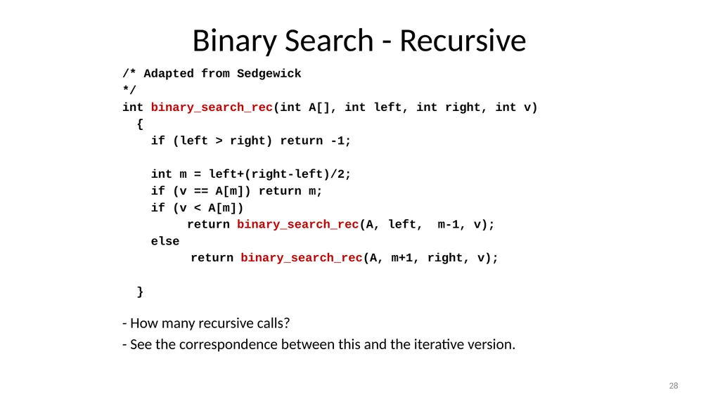
slide28. Binary Search - Recursive /* Adapted from Sedgewick
*/
int binary_search_rec(int A[], int left, int right, int v)
{
if (left > right) return -1;
int m = left+(right-left)/2;
if (v == A[m]) return m;
if (v < A[m])
return binary_search_rec(A, left, m-1, v);
else
return binary_search_rec(A, m+1, right, v);
}
- How many recursive calls?
- See the correspondence between this and the iterative version. 28<br>
slide29. Interpolated search covered if time permits 29<br>
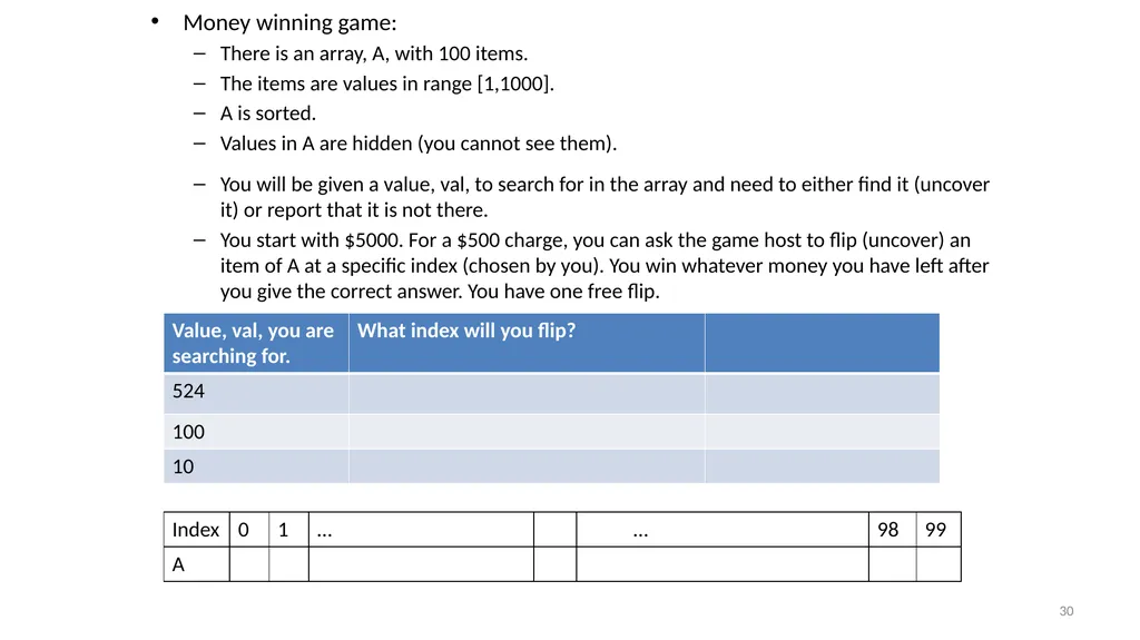
slide30. Money winning game:
There is an array, A, with 100 items.
The items are values in range [1,1000].
A is sorted.
Values in A are hidden (you cannot see them).
You will be given a value, val, to search for in the array and need to either find it (uncover it) or report that it is not there.
You start with $5000. For a $500 charge, you can ask the game host to flip (uncover) an item of A at a specific index (chosen by you). You win whatever money you have left after you give the correct answer. You have one free flip. 30<br>
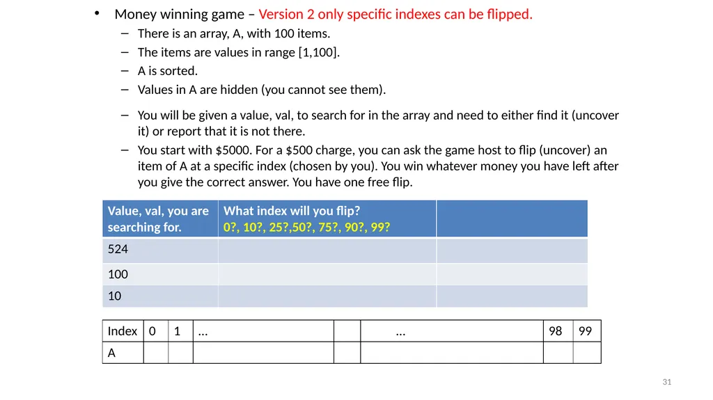
slide31. Money winning game – Version 2 only specific indexes can be flipped.
There is an array, A, with 100 items.
The items are values in range [1,100].
A is sorted.
Values in A are hidden (you cannot see them).
You will be given a value, val, to search for in the array and need to either find it (uncover it) or report that it is not there.
You start with $5000. For a $500 charge, you can ask the game host to flip (uncover) an item of A at a specific index (chosen by you). You win whatever money you have left after you give the correct answer. You have one free flip. 31<br>
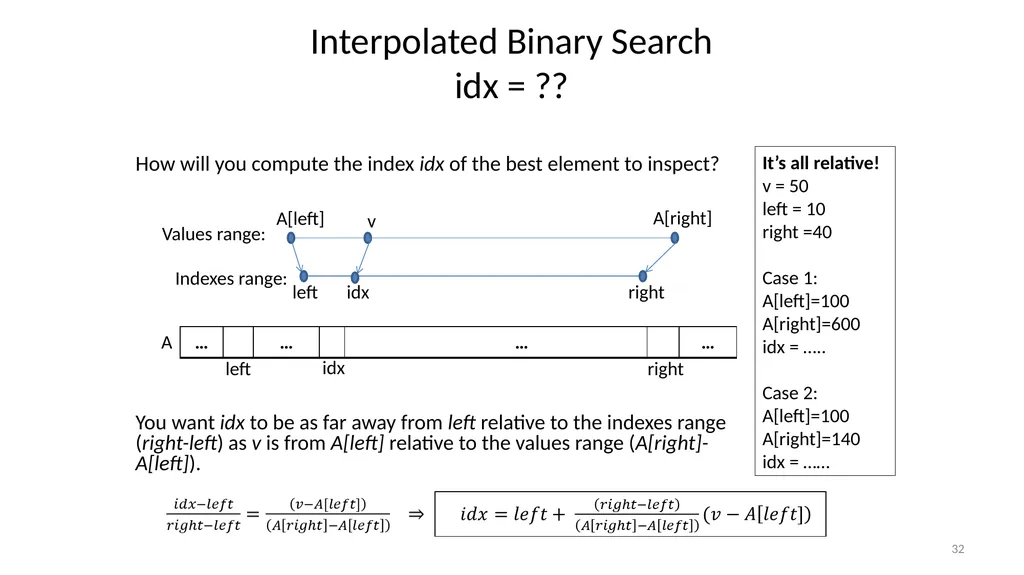
slide32. Interpolated Binary Search idx = ?? 32 A[left] A[right] left right idx v left right idx Values range: Indexes range: A How will you compute the index idx of the best element to inspect? You want idx to be as far away from left relative to the indexes range (right-left) as v is from A[left] relative to the values range (A[right]-A[left]). It’s all relative!
v = 50
left = 10
right =40
Case 1:
A[left]=100
A[right]=600
idx = …..
Case 2:
A[left]=100
A[right]=140
idx = ……<br>
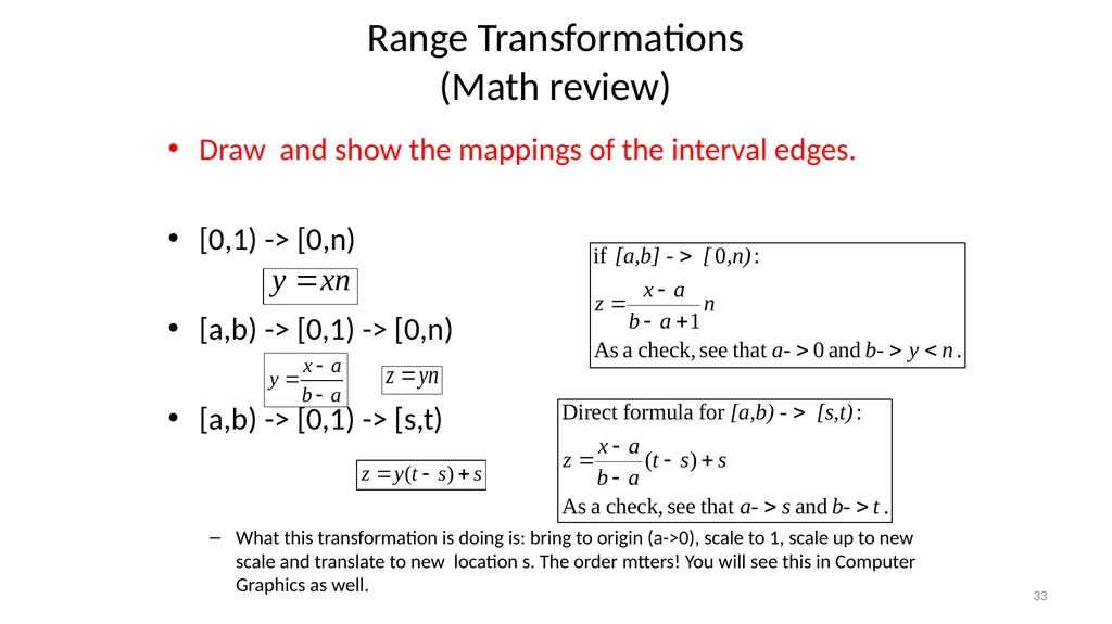
slide33. Range Transformations (Math review) Draw and show the mappings of the interval edges.
[0,1) -> [0,n)
[a,b) -> [0,1) -> [0,n)
[a,b) -> [0,1) -> [s,t)
What this transformation is doing is: bring to origin (a->0), scale to 1, scale up to new scale and translate to new location s. The order mtters! You will see this in Computer Graphics as well. 33<br>
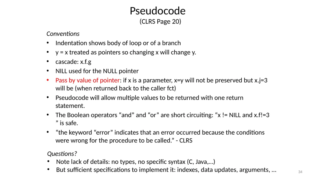
slide34. Pseudocode (CLRS Page 20) Conventions
Indentation shows body of loop or of a branch
y = x treated as pointers so changing x will change y.
cascade: x.f.g
NILL used for the NULL pointer
Pass by value of pointer: if x is a parameter, x=y will not be preserved but x.j=3 will be (when returned back to the caller fct)
Pseudocode will allow multiple values to be returned with one return statement.
The Boolean operators “and” and “or” are short circuiting: “x != NILL and x.f!=3 ” is safe.
“the keyword “error” indicates that an error occurred because the conditions were wrong for the procedure to be called.” - CLRS 34 Questions?
Note lack of details: no types, no specific syntax (C, Java,…)
But sufficient specifications to implement it: indexes, data updates, arguments, …<br>
Insertion Sort
Binary Search CSE 3318 – Algorithms and Data Structures
Alexandra Stefan
University of Texas at Arlington 1 1/16/2025<br>
slide2. Summary Properties of sorting algorithms
Sorting algorithms
Insertion sort – Chapter 2 (CLRS)
Indirect sorting - (Sedgewick Ch. 6.8 ‘Index and Pointer Sorting’)
Binary Search
See the notation conventions (e.g. log2N = lg N)
Terminology and notation:
log2N = lg N
Use interchangeably:
Runtime and time complexity
Record and item 2<br>
slide3. Sorting 3<br>
slide4. Sorting Sort an array, A, of items (numbers, strings, etc.).
Why sort it?
To use in binary search.
To compute rankings, statistics (min/max, top-10, top-100, median).
Check that there are no duplicates
intersection and union are easier to perform between 2 sorted sets
….
We will study several sorting algorithms,
Pros/cons, behavior .
Insertion sort
Optional, self study: selection sort. 4<br>
slide5. Properties of sorting Stable:
It does not change the relative order of items whose keys are equal.
Adaptive:
The time complexity will depend on the input
E.g. if the input data is almost sorted, it will run significantly faster than if not sorted.
see later insertion sort vs selection sort. 5<br>
slide6. Other aspects of sorting Time complexity: worst/best/average
Number of data moves: copy/swap the DATA RECORDS
One data move = 1 copy operation of a complete data record
Data moves are NOT updates of variables independent of record size (e.g. loop counter )
Space complexity: Extra Memory used
Do NOT count the space needed to hold the INPUT data, only extra space (e.g. copy of data)
Θ(1): In place methods: constant extra memory
Θ(N): Uses extra space proportional to the number of items:
For pointers (e.g. linked lists or indirect access)
For a copy of the data
Direct vs indirect sorting
Direct: move items as needed to sort
Indirect: move pointers/handles to items.
Can keep the key with pointer or not.
Later: non-comparison sorting 6<br>
slide7. Stable sorting A sorting algorithm is stable iff, after it sorts an array, any two records that compare equal, will still be in the same relative order as they were before sorting and this happens for every possible input array.
Example:
An item consists of an int (e.g. GPA) and a string (e.g. name).
Sort based on: GPA (integer)
Stable sort (OK: Tom before Jane and Bob before Anna):
Unstable sort (violation: Anna is now before Bob):
Note: Stable is a property of the algorithm, NOT of the algorithm-data pair. You CANNOT say “This algorithm is stable for this input”. It must be so for all inputs. 7<br>
slide8. Stable sorting - Application Applications
Sorting by 2 criteria,
E.g.: 1st by GPA, 2nd by name:
When the GPA is the same, have data in order of names
Solution:
First sort by name (with any method)
Next, with a stable sort, sort by GPA
Alternative solution:
write a more complex comparison function.
Part of other sorting methods
See later: LSD radix sort uses a stable sort (count sort). 8<br>
slide9. Proving an Algorithm is Stable An algorithm is stable if we can guarantee/prove that this property happens for any input (not just a few example inputs).
=> To prove it, must use an actual proof (possibly using a loop invariant) or give a very good explanation. Checking that “it works” on a few examples is NOT a proof. It must work for every possible input that is valid.
An algorithm is not stable if there is at least one possible input for which it breaks the property.
=> To prove it, find one example input for which the property fails.
=> easier to prove.
Intuition: if an algorithm swaps items that are away from each other (jump over other items) it is most likely NOT stable.
This statement is a guideline, not a proof. Make sure you always find an example if you suspect this case. 9<br>
slide10. Insertion sort 10<br>
slide11. Insertion sort 11 Each row shows the array after one iteration of the outer loop (after step j). Process the array from left to right.
Step j (outer loop):
- elements A[0],A[1],…A[j-1] are already sorted
- insert element A[j] in it’s place among A[0],..A[j-1] (inner loop) Elements in shaded cells are sorted, but they have only items that were originally in the shaded cells. They are not in final position (e.g. see the 8 move all the way to the right). See TedEd video
Wikipedia (see “A graphical example of insertion sort”): https://en.wikipedia.org/wiki/Insertion_sort
Brief and nice resource: http://interactivepython.org/runestone/static/pythonds/SortSearch/TheInsertionSort.html
Animation for version that swaps elements: https://youtu.be/Q1JdRUh1_98 (sent by Aryan)<br>
slide12. Insertion Sort 12 Repetition of while-k
At most: j (Includes end loop check)
At least: 1 (Evaluate:(k>0 and A[k]>key) ) void insertion_sort(int A[],int N){
int j,k,curr;
for (j=1; j<N; j++){
curr = A[j];
// insert curr (A[j]) in the
// sorted sequence A[0…j-1]
k = j-1;
while ((k>=0) && (A[k]>curr)){
A[k+1] = A[k];
k = k–1;
}
A[k+1] = curr;
} ‘Data move’ is an assignment.
(matters if deep copy or pointer is used)
Each red number: 2 moves.
Each blue number: 1 move.
Best: Θ(N)
Worst: Θ(N2) Average: Θ(N2)<br>
slide13. Insertion Sort Time Complexity 13 ‘Total’ instructions in worst case:
(N-1) + (N-2) + … 2 + 1 =
= [N * (N-1)]/2 -> Θ(N2)
Note that the N2 came from the summation, NOT because ‘there is an N in the inner loop’ (NOT because N * N). => O(N2) “O” will be explained in detail later. It says that the algorithm take at most order of N2.
See the Khan Academy for a discussion on the use of O(N2):
https://www.khanacademy.org/computing/computer-science/algorithms/insertion-sort/a/insertion-sort Insertion sort is adaptive void insertion_sort(int A[],int N){
int j,k, curr;
for (j=1; j<N; j++){
curr = A[j];
// insert curr (A[j]) in the
// sorted sequence A[0…j-1]
k = j-1;
while ((k>=0) && (A[k]>curr)){
A[k+1] = A[k];
k = k–1;
}
A[k+1] = curr;
}<br>
slide14. Insertion sort: Time Complexity & Data moves 14 Time complexity Each row shows the array after one iteration of the outer loop for each algorithm.
‘Data move’ is an assignment. (Implementation will matter: deep copy or pointer)
Each row shows the array after one iteration of the outer loop for each algorithm. Insert the next element in it’s place in the sorted sequence to the left of it. Gray cells are visited by the iterations of the inner loop => they are proportional with the time complexity => ~ N2/2 (worst case) Data moves Insert the next element in it’s place in the sorted sequence to the left of it. Each red number: 2 moves.
Each blue number: 1 move.
Best: 2(N-1) Worst: 2(N-1)+N(N-1)/2 Average:2N+N(N-1)/4<br>
slide15. Insertion sort - Properties Time complexity: O(N2) (Θ(N) – best, Θ(N2) – worst and average )
Space complexity: Θ(1) (it does not copy any of array)
Data moves: Θ(N) – best, Θ(N2) – worst and average
Adaptive: Yes (Θ(N) – best case, Θ(N2) – worst and average case)
Stable – Yes
Direct sorting 15<br>
slide16. Insertion sort - Variations Note how an algorithm has the capability to be stable but the way it is implemented can still make it unstable.
What happens if we use A[k]>=key in line 5?
Give an implementation that uses a sentinel (to avoid the k>0 check in line 5)
What is a sentinel?
Is it still stable? (How do you update/move the sentinel)?
Time complexity trade-off:
Cost to set-up the sentinel (linear: find the smallest element in the array) vs
Savings from removing the k>0 check (quadratic, in worst case). 16<br>
slide17. Proving That an Algorithm is Correct Required. Read the relevant book section if needed.
See CLRS, (starting at page 18), for proof of loop invariant and correctness of the insertion sort algorithm:
Identify a property that is preserved (maintained, built) by the algorithm: “the loop invariant” (b.c. preserved by the loop)
Which loop would you use here?
Show:
Initialization: it is true prior to the 1st iteration
Maintenance (j->j+1): If it is true before an iteration it remains true before the next iteration
Termination – use that property/invariant to show that the algorithm is correct
What would the loop invariant be for the inner loop for insertion sort?
This question may be part of your next homework or quiz. 17<br>
slide18. Indirect Sorting What if we need access to our data (array/list) in sorted order but
do not want to move records around
records are too big
records are already sorted by another criterion and we need that too.
cannot move records around.
only have read access, but no write access
Solution: Indirect sorting
Generate a new array with references (e.g. indexes) to records in sorted order. 18<br>
slide19. Indirect Sorting 19 Data[ X[0] ] The i-th element in sorted order is given by Data[Idxs[i]] for (j=0; j<7; j++){
printf("%d\n", Data[ X[j] ] );
}<br>
slide20. Indirect Sorting 20 Data[ X[0] ] The i-th element in sorted order is given by Data[Idxs[i]] “Sort” X with insertion sort Create the identity array, X, with indexes 0 to N-1
Adapt insertion sort to rearrange the elements of X
What do you copy?
What do you compare?
Return X
Language specific issues (C/Java)
Access Data through X: e.g. Data[ X[j] ] void insertion_sort(int A[],int N){
int j,k,curr;
for (j=1; j<N; j++){
curr = A[j];
k = j-1;
while ((k>=0) && ( A[k] > curr) ){
A[k+1] = A[k];
k = k–1;
}
A[k+1] = curr;
}<br>
slide21. Indirect Sorting Food for thought:
Example of references:
indexes
memory addresses
offsets in a file
Can we indirect sort a linked list? 21<br>
slide22. Binary Search and Indirect Sorting 22<br>
slide23. Binary Search and Indirect Sorting 23 Data[ X[0] ] The j-th element in sorted order is given by Data[X[j]] 1. int search(int A[], int N, int v){
2. int left, right;
3. left = 0; right = N-1;
4. while (left <= right)
5. { int m = left+(right-left)/2;
6. if (v == A[m]) return m;
7. if (v < A[m])
8. right = m-1;
9. else
10. left = m+1;
11. }
12. return -1;
13. } use binary search to
search for values:
115
950
250<br>
slide24. Binary Search and Indirect Sorting 24 Data[ X[0] ] The j-th element in sorted order is given by Data[X[j]] 1. int search(int A[], int N, int v){
2. int left, right;
3. left = 0; right = N-1;
4. while (left <= right)
5. { int m = left+(right-left)/2;
6. if (v == A[m]) return m;
7. if (v < A[m])
8. right = m-1;
9. else
10. left = m+1;
11. }
12. return -1;
13. } use binary search to
search for values:
115
950
250<br>
slide25. Binary Search 25<br>
slide26. Binary Search Iterative Search for 392 in sorted array.
v = 392 26 /* Determines if v is an element of A.
If yes, returns the position of v in A.
If not, returns -1. N is the size of A */
1. int binary_search(int A[], int N, int v){
2. int left, right;
3. left = 0; right = N-1;
4. while (left <= right) {
5. int m = left+(right-left)/2;
6. if (v == A[m]) return m;
7. if (v < A[m])
8. right = m-1;
9. else
10. left = m+1;
11. }
12. return -1;
13. } Problem: Determine if object v is in array A. Assume A has size N and is sorted in ascending order.
Reduces the search range in half, with a few instructions.
See animation: https://www.cs.usfca.edu/~galles/visualization/Search.html
The array stretches on 2 or more lines<br>
slide27. Binary Search Search for v=392 in sorted array: 27 /* code from Sedgewick
Determines if v is an element of A.
If yes, returns the position of v in A.
If not, returns -1. N is the size of A.
*/
1. int binary_search(int A[], int N, int v){
2. int left, right;
3. left = 0; right = N-1;
4. while (left <= right) {
5. int m = left+(right-left)/2;
6. if (v == A[m]) return m;
7. if (v < A[m])
8. right = m-1;
9. else
10. left = m+1;
11. }
12. return -1;
13. } Candidates: N, N/2, N/(22) , N/(23), …. , , N/(2x), …., N/(2p) =1 (last value for which the loop will start) => p = log2N => log2N repetitions
TC1iter() = Θ(1), indep of current number of candiates = right-left+1) =>
Time complexity: Θ(log2N) (logarithmic. V is compared with at most log2N items.
Space complexity: Θ(1)<br>
slide28. Binary Search - Recursive /* Adapted from Sedgewick
*/
int binary_search_rec(int A[], int left, int right, int v)
{
if (left > right) return -1;
int m = left+(right-left)/2;
if (v == A[m]) return m;
if (v < A[m])
return binary_search_rec(A, left, m-1, v);
else
return binary_search_rec(A, m+1, right, v);
}
- How many recursive calls?
- See the correspondence between this and the iterative version. 28<br>
slide29. Interpolated search covered if time permits 29<br>
slide30. Money winning game:
There is an array, A, with 100 items.
The items are values in range [1,1000].
A is sorted.
Values in A are hidden (you cannot see them).
You will be given a value, val, to search for in the array and need to either find it (uncover it) or report that it is not there.
You start with $5000. For a $500 charge, you can ask the game host to flip (uncover) an item of A at a specific index (chosen by you). You win whatever money you have left after you give the correct answer. You have one free flip. 30<br>
slide31. Money winning game – Version 2 only specific indexes can be flipped.
There is an array, A, with 100 items.
The items are values in range [1,100].
A is sorted.
Values in A are hidden (you cannot see them).
You will be given a value, val, to search for in the array and need to either find it (uncover it) or report that it is not there.
You start with $5000. For a $500 charge, you can ask the game host to flip (uncover) an item of A at a specific index (chosen by you). You win whatever money you have left after you give the correct answer. You have one free flip. 31<br>
slide32. Interpolated Binary Search idx = ?? 32 A[left] A[right] left right idx v left right idx Values range: Indexes range: A How will you compute the index idx of the best element to inspect? You want idx to be as far away from left relative to the indexes range (right-left) as v is from A[left] relative to the values range (A[right]-A[left]). It’s all relative!
v = 50
left = 10
right =40
Case 1:
A[left]=100
A[right]=600
idx = …..
Case 2:
A[left]=100
A[right]=140
idx = ……<br>
slide33. Range Transformations (Math review) Draw and show the mappings of the interval edges.
[0,1) -> [0,n)
[a,b) -> [0,1) -> [0,n)
[a,b) -> [0,1) -> [s,t)
What this transformation is doing is: bring to origin (a->0), scale to 1, scale up to new scale and translate to new location s. The order mtters! You will see this in Computer Graphics as well. 33<br>
slide34. Pseudocode (CLRS Page 20) Conventions
Indentation shows body of loop or of a branch
y = x treated as pointers so changing x will change y.
cascade: x.f.g
NILL used for the NULL pointer
Pass by value of pointer: if x is a parameter, x=y will not be preserved but x.j=3 will be (when returned back to the caller fct)
Pseudocode will allow multiple values to be returned with one return statement.
The Boolean operators “and” and “or” are short circuiting: “x != NILL and x.f!=3 ” is safe.
“the keyword “error” indicates that an error occurred because the conditions were wrong for the procedure to be called.” - CLRS 34 Questions?
Note lack of details: no types, no specific syntax (C, Java,…)
But sufficient specifications to implement it: indexes, data updates, arguments, …<br>