
SORTING OVERVIEW 1) Why do we need sorting


Description: SORTING OVERVIEW 1) Why do we need sorting algorithms? 2) Simple sorting algorithms 3) More complicated sorting algorithms 4) Distribution sorts 1) Why do we need sorting algorithms? Sorting can help avoid repeating data any repeating
Related Topics
Download Presentation
"SORTING OVERVIEW 1) Why do we need sorting" is the property of its rightful owner. Permission is granted to download and print the materials on this website for personal, non-commercial use only, and to display it on your personal computer provided you do not modify the materials and that you retain all copyright notices contained in the materials. By downloading content from our website, you accept the terms of this agreement.
Presentation Transcript
slide1. SORTING<br>
slide2. OVERVIEW 1) Why do we need sorting algorithms?
2) Simple sorting algorithms
3) More complicated sorting algorithms
4) Distribution sorts<br>
slide3. 1) Why do we need sorting algorithms? Sorting can help avoid repeating data – any repeating data will be placed together within a sorted array and can thus be easily removed if necessary
Searching through data is made faster: without sorting, every value must be checked, however, sorted arrays allow for faster searches such as binary searching, which does not look at every value
Sets of data can be easily compared when both sets are ordered – it is easy to see where the sets of data have the same and different values.<br>
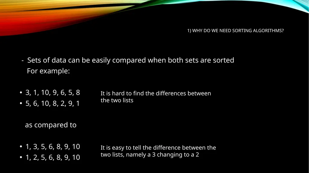
slide4. - Sets of data can be easily compared when both sets are sorted
For example:
3, 1, 10, 9, 6, 5, 8
5, 6, 10, 8, 2, 9, 1
as compared to
1, 3, 5, 6, 8, 9, 10
1, 2, 5, 6, 8, 9, 10 It is hard to find the differences between the two lists It is easy to tell the difference between the two lists, namely a 3 changing to a 2 1) Why do we need sorting algorithms?<br>
slide5. 2) Simple sorting algorithms SELECTION SORT
Selection Sort works by finding the smallest value in an array, and then placing that value at the start of the array. It then repeats with the second smallest value, and so on, until you have a sorted array
The sort is easy to code, however, due to its O(n²) time complexity, it should not be used to sort large arrays, nor should it be used when the speed of the algorithm is important<br>
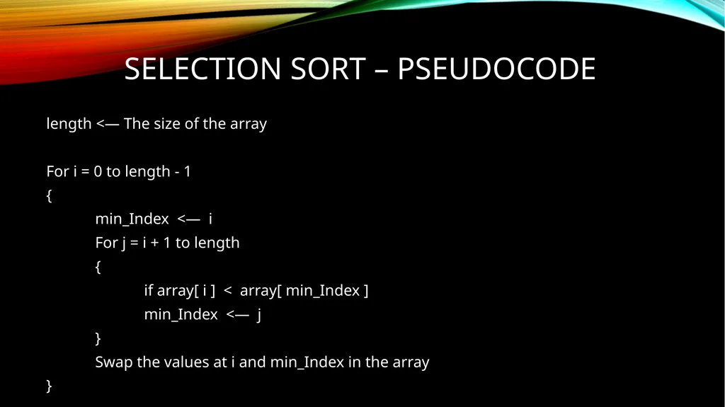
slide6. Selection sort – pseudocode length <— The size of the array
For i = 0 to length - 1
{
min_Index <— i
For j = i + 1 to length
{
if array[ i ] < array[ min_Index ]
min_Index <— j
}
Swap the values at i and min_Index in the array
}<br>
slide7. 2) Simple sorting algorithms BUBBLE SORT
Bubble Sort works by comparing every adjacent pair of numbers and swapping them if the larger number is positioned first. This is repeated n times (where n is the number of elements in the array)
Once again, this sort is easy to code and has a time complexity of O(n²). Because more swaps take place than the selection sort, this sort is less efficient and should not be used to sort large arrays
This sort can be fast when used on a nearly sorted array, assuming it has been coded to have a flag (the sort stops when no more changes are being made)<br>
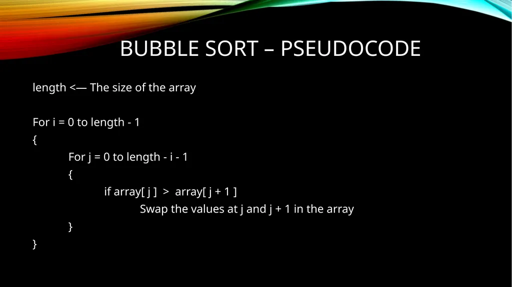
slide8. BUBBLE sort – pseudocode length <— The size of the array
For i = 0 to length - 1
{
For j = 0 to length - i - 1
{
if array[ j ] > array[ j + 1 ]
Swap the values at j and j + 1 in the array
}
}<br>
slide9. 3) More complicated sorting algorithms MERGE SORT
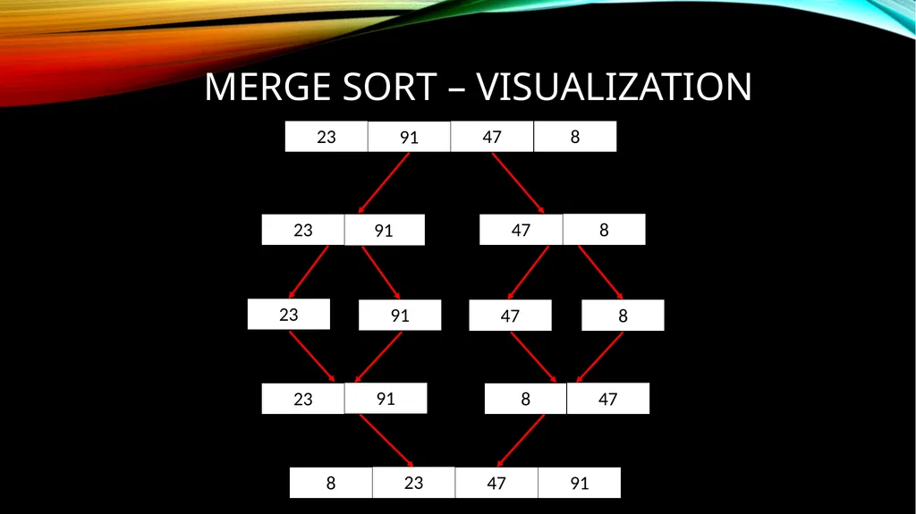
Merge Sort works by breaking an array into sub-arrays, each containing an individual element. Every 2 sub-arrays are merged to make a larger, ordered sub-array. Those sub-arrays are once again merged, and this continues until there is only one array, the final sorted array.
This sort is much more complicated to code, and has a time complexity of O(n log n), making it much better to use for large amounts of data.<br>
slide10. Merge sort – visualization 91 23 47 8 91 23 47 8 23 91 47 8 91 23 8 47 23 8 47 91<br>
slide11. 3) More complicated sorting algorithms QUICK SORT
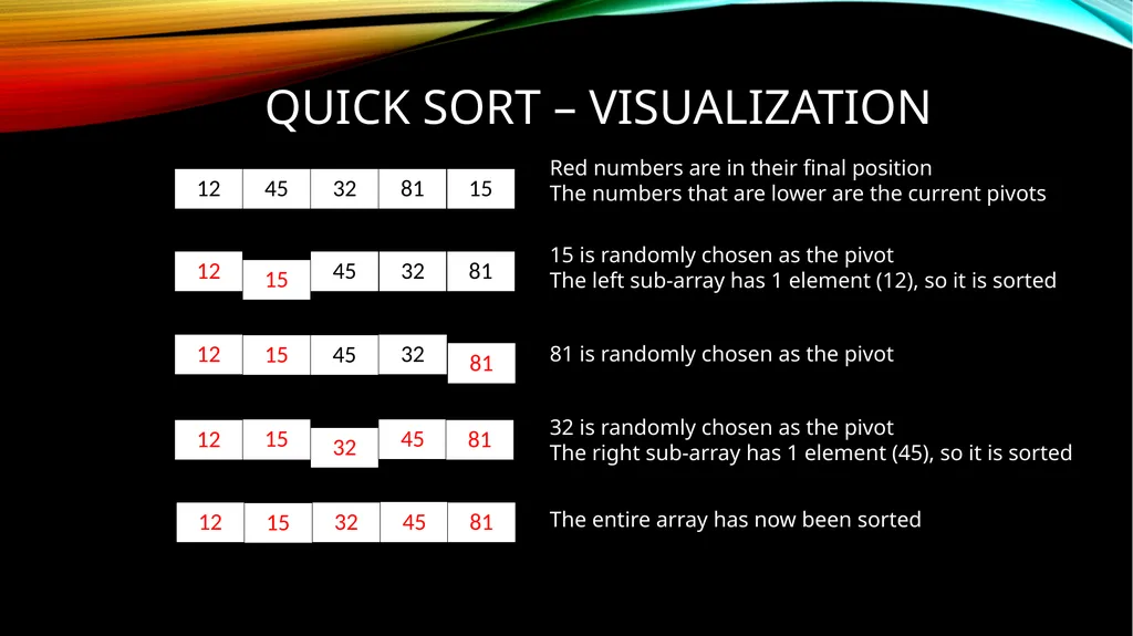
Quick Sort works by choosing a pivot and then separating every value greater than the pivot from every value smaller than the pivot, making two smaller sub-arrays. At this point, the pivot is in its final location. Quicksort is then recursively called on these sub-arrays, until every element is in the correct order
Quicksort is often considered the most efficient sorting algorithm. It is part of the hybrid sort used in the C++ sort() function (Introsort) and is also used in the java Arrays.sort() function.
The time complexity is on average O(n log n); however, the worst case is O(n²) (although this case is unlikely when pivots are chosen at random)<br>
slide12. Quick sort – visualization 12 45 32 81 15 12 45 32 81 15 12 45 32 81 15 12 45 32 81 15 12 45 32 81 15 Red numbers are in their final position
The numbers that are lower are the current pivots 15 is randomly chosen as the pivot
The left sub-array has 1 element (12), so it is sorted 81 is randomly chosen as the pivot 32 is randomly chosen as the pivot
The right sub-array has 1 element (45), so it is sorted The entire array has now been sorted<br>
slide13. 4) Distribution sorts COUNTING SORT
Distribution sorts work by moving data from the input into multiple structures, and then collecting them at the output, instead of comparing the values themselves.
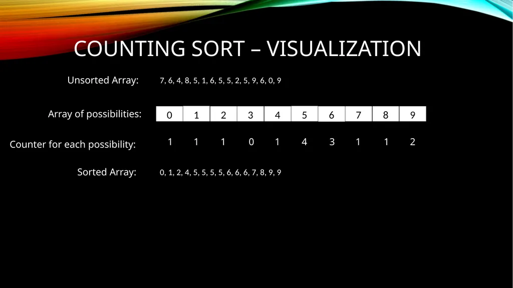
Counting Sort works by counting the number of times every number is found inside an array, and then displaying each number based on the number of times it was counted
This sort can be extremely efficient but becomes less efficient the greater the size of the set of possible numbers is. The sort also only works when every number falls within a particular set of possibilities
The time complexity is O(n + k), where k is the range of the possible values<br>
slide14. 0 1 2 3 4 5 6 7 8 9 7, 6, 4, 8, 5, 1, 6, 5, 5, 2, 5, 9, 6, 0, 9 Counting sort – visualization Array of possibilities: Counter for each possibility: Unsorted Array: 1 1 1 0 1 4 3 1 1 2 0, 1, 2, 4, 5, 5, 5, 5, 6, 6, 6, 7, 8, 9, 9 Sorted Array:<br>
slide15. 4) Distribution sorts RADIX SORT
Radix Sort works by splitting the numbers into ‘buckets’ based on an individual digit. For example, using a base 10 radix sort, there will be 10 buckets for the digits 0 – 9. First, the numbers are grouped based on their least significant digit (LSD) and then combined back into an array one bucket at a time. Then they are sorted by the second least significant digit, then the third, until the most significant digit (MSD).
This sort is more complicated to code than the earlier mentioned simpler algorithms and has a time complexity of O(n * k), where k is the number of digits in the largest number.<br>
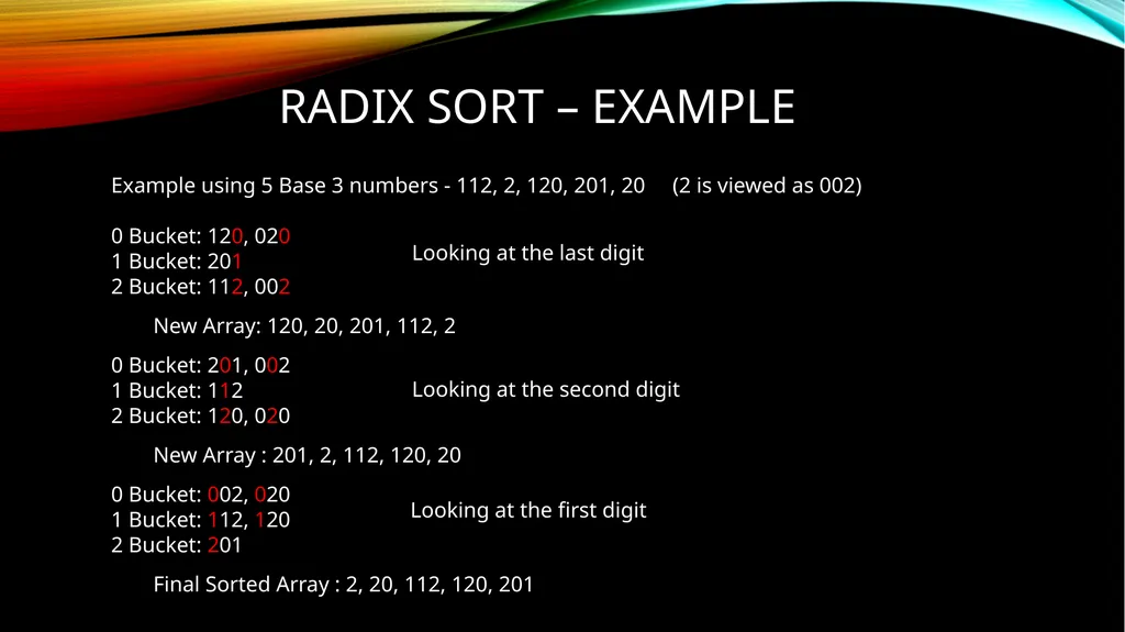
slide16. radix sort – Example Example using 5 Base 3 numbers - 112, 2, 120, 201, 20 (2 is viewed as 002)
0 Bucket: 120, 020
1 Bucket: 201
2 Bucket: 112, 002
New Array: 120, 20, 201, 112, 2
0 Bucket: 201, 002
1 Bucket: 112
2 Bucket: 120, 020
New Array : 201, 2, 112, 120, 20
0 Bucket: 002, 020
1 Bucket: 112, 120
2 Bucket: 201
Final Sorted Array : 2, 20, 112, 120, 201 Looking at the last digit Looking at the second digit Looking at the first digit<br>
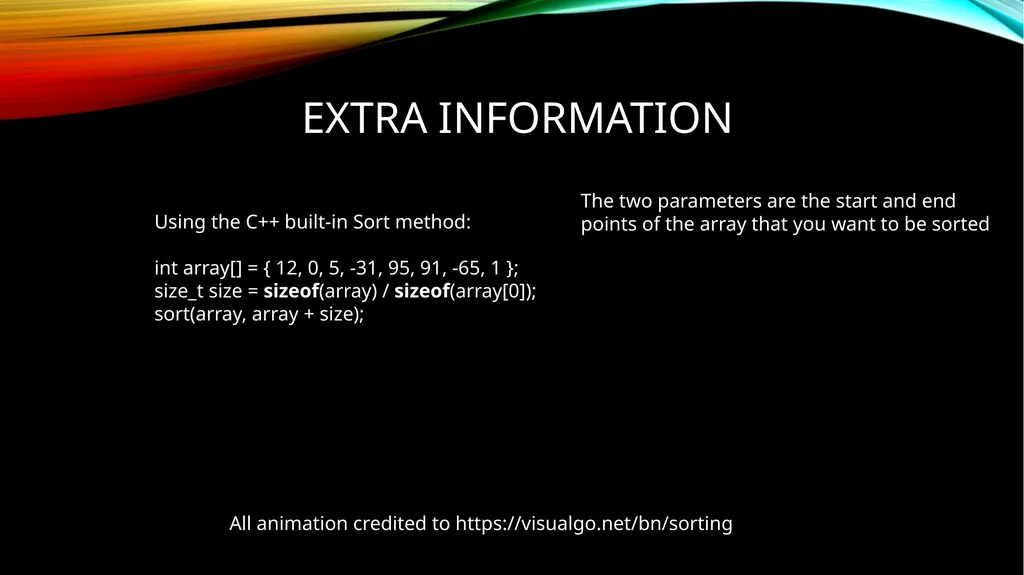
slide17. All animation credited to https://visualgo.net/bn/sorting Extra information Using the C++ built-in Sort method:
int array[] = { 12, 0, 5, -31, 95, 91, -65, 1 };
size_t size = sizeof(array) / sizeof(array[0]);
sort(array, array + size); The two parameters are the start and end points of the array that you want to be sorted<br>
slide2. OVERVIEW 1) Why do we need sorting algorithms?
2) Simple sorting algorithms
3) More complicated sorting algorithms
4) Distribution sorts<br>
slide3. 1) Why do we need sorting algorithms? Sorting can help avoid repeating data – any repeating data will be placed together within a sorted array and can thus be easily removed if necessary
Searching through data is made faster: without sorting, every value must be checked, however, sorted arrays allow for faster searches such as binary searching, which does not look at every value
Sets of data can be easily compared when both sets are ordered – it is easy to see where the sets of data have the same and different values.<br>
slide4. - Sets of data can be easily compared when both sets are sorted
For example:
3, 1, 10, 9, 6, 5, 8
5, 6, 10, 8, 2, 9, 1
as compared to
1, 3, 5, 6, 8, 9, 10
1, 2, 5, 6, 8, 9, 10 It is hard to find the differences between the two lists It is easy to tell the difference between the two lists, namely a 3 changing to a 2 1) Why do we need sorting algorithms?<br>
slide5. 2) Simple sorting algorithms SELECTION SORT
Selection Sort works by finding the smallest value in an array, and then placing that value at the start of the array. It then repeats with the second smallest value, and so on, until you have a sorted array
The sort is easy to code, however, due to its O(n²) time complexity, it should not be used to sort large arrays, nor should it be used when the speed of the algorithm is important<br>
slide6. Selection sort – pseudocode length <— The size of the array
For i = 0 to length - 1
{
min_Index <— i
For j = i + 1 to length
{
if array[ i ] < array[ min_Index ]
min_Index <— j
}
Swap the values at i and min_Index in the array
}<br>
slide7. 2) Simple sorting algorithms BUBBLE SORT
Bubble Sort works by comparing every adjacent pair of numbers and swapping them if the larger number is positioned first. This is repeated n times (where n is the number of elements in the array)
Once again, this sort is easy to code and has a time complexity of O(n²). Because more swaps take place than the selection sort, this sort is less efficient and should not be used to sort large arrays
This sort can be fast when used on a nearly sorted array, assuming it has been coded to have a flag (the sort stops when no more changes are being made)<br>
slide8. BUBBLE sort – pseudocode length <— The size of the array
For i = 0 to length - 1
{
For j = 0 to length - i - 1
{
if array[ j ] > array[ j + 1 ]
Swap the values at j and j + 1 in the array
}
}<br>
slide9. 3) More complicated sorting algorithms MERGE SORT
Merge Sort works by breaking an array into sub-arrays, each containing an individual element. Every 2 sub-arrays are merged to make a larger, ordered sub-array. Those sub-arrays are once again merged, and this continues until there is only one array, the final sorted array.
This sort is much more complicated to code, and has a time complexity of O(n log n), making it much better to use for large amounts of data.<br>
slide10. Merge sort – visualization 91 23 47 8 91 23 47 8 23 91 47 8 91 23 8 47 23 8 47 91<br>
slide11. 3) More complicated sorting algorithms QUICK SORT
Quick Sort works by choosing a pivot and then separating every value greater than the pivot from every value smaller than the pivot, making two smaller sub-arrays. At this point, the pivot is in its final location. Quicksort is then recursively called on these sub-arrays, until every element is in the correct order
Quicksort is often considered the most efficient sorting algorithm. It is part of the hybrid sort used in the C++ sort() function (Introsort) and is also used in the java Arrays.sort() function.
The time complexity is on average O(n log n); however, the worst case is O(n²) (although this case is unlikely when pivots are chosen at random)<br>
slide12. Quick sort – visualization 12 45 32 81 15 12 45 32 81 15 12 45 32 81 15 12 45 32 81 15 12 45 32 81 15 Red numbers are in their final position
The numbers that are lower are the current pivots 15 is randomly chosen as the pivot
The left sub-array has 1 element (12), so it is sorted 81 is randomly chosen as the pivot 32 is randomly chosen as the pivot
The right sub-array has 1 element (45), so it is sorted The entire array has now been sorted<br>
slide13. 4) Distribution sorts COUNTING SORT
Distribution sorts work by moving data from the input into multiple structures, and then collecting them at the output, instead of comparing the values themselves.
Counting Sort works by counting the number of times every number is found inside an array, and then displaying each number based on the number of times it was counted
This sort can be extremely efficient but becomes less efficient the greater the size of the set of possible numbers is. The sort also only works when every number falls within a particular set of possibilities
The time complexity is O(n + k), where k is the range of the possible values<br>
slide14. 0 1 2 3 4 5 6 7 8 9 7, 6, 4, 8, 5, 1, 6, 5, 5, 2, 5, 9, 6, 0, 9 Counting sort – visualization Array of possibilities: Counter for each possibility: Unsorted Array: 1 1 1 0 1 4 3 1 1 2 0, 1, 2, 4, 5, 5, 5, 5, 6, 6, 6, 7, 8, 9, 9 Sorted Array:<br>
slide15. 4) Distribution sorts RADIX SORT
Radix Sort works by splitting the numbers into ‘buckets’ based on an individual digit. For example, using a base 10 radix sort, there will be 10 buckets for the digits 0 – 9. First, the numbers are grouped based on their least significant digit (LSD) and then combined back into an array one bucket at a time. Then they are sorted by the second least significant digit, then the third, until the most significant digit (MSD).
This sort is more complicated to code than the earlier mentioned simpler algorithms and has a time complexity of O(n * k), where k is the number of digits in the largest number.<br>
slide16. radix sort – Example Example using 5 Base 3 numbers - 112, 2, 120, 201, 20 (2 is viewed as 002)
0 Bucket: 120, 020
1 Bucket: 201
2 Bucket: 112, 002
New Array: 120, 20, 201, 112, 2
0 Bucket: 201, 002
1 Bucket: 112
2 Bucket: 120, 020
New Array : 201, 2, 112, 120, 20
0 Bucket: 002, 020
1 Bucket: 112, 120
2 Bucket: 201
Final Sorted Array : 2, 20, 112, 120, 201 Looking at the last digit Looking at the second digit Looking at the first digit<br>
slide17. All animation credited to https://visualgo.net/bn/sorting Extra information Using the C++ built-in Sort method:
int array[] = { 12, 0, 5, -31, 95, 91, -65, 1 };
size_t size = sizeof(array) / sizeof(array[0]);
sort(array, array + size); The two parameters are the start and end points of the array that you want to be sorted<br>