Species interaction models Goal Determine whether a site is occupied by two different species and if they affect each others detection and occupancy probabilities. Examples Predator-prey interactions Competitive exclusion Compares:
"Species interaction models Goal Determine whether" is the property of its rightful owner. Permission is granted to
download and print the materials on this website for personal, non-commercial use only, and to display it
on your personal computer provided you do not modify the materials and that you retain all copyright
notices contained in the materials. By downloading content from our website, you accept the terms of this
agreement.
Presentation Transcript
01
Species interaction models<br>
02
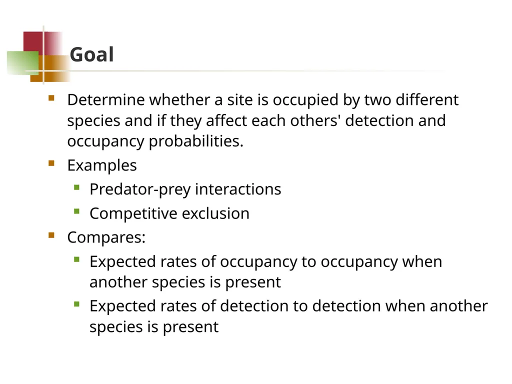
Goal Determine whether a site is occupied by two different species and if they affect each others' detection and occupancy probabilities.
Examples
Predator-prey interactions
Competitive exclusion
Compares:
Expected rates of occupancy to occupancy when another species is present
Expected rates of detection to detection when another species is present<br>
03
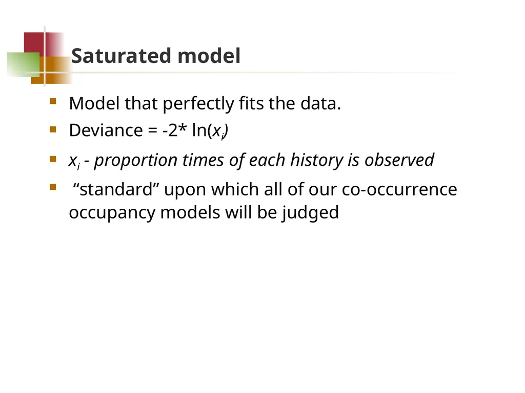
Saturated model Model that perfectly fits the data.
Deviance = -2*ln(xi)
xi - proportion times of each history is observed
“standard” upon which all of our co-occurrence occupancy models will be judged<br>
04
Similarities to single season occupancy Relates encounter histories and detection probabilities to a site.
Occupancy is assumed closed during sampling period
Site is sampled multiple times
Encounter history is obtained for both species
Based on repeated sampling
Spatial or temporal replication<br>
05
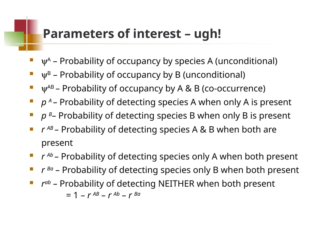
Parameters of interest – ugh! yA – Probability of occupancy by species A (unconditional)
yB – Probability of occupancy by B (unconditional)
yAB – Probability of occupancy by A & B (co-occurrence)
p A – Probability of detecting species A when only A is present
p B– Probability of detecting species B when only B is present
r AB – Probability of detecting species A & B when both are present
r Ab – Probability of detecting species only A when both present
r Ba – Probability of detecting species only B when both present
rab – Probability of detecting NEITHER when both present = 1 – r AB – r Ab – r Ba<br>
06
Many parameters = much data required!<br>
07
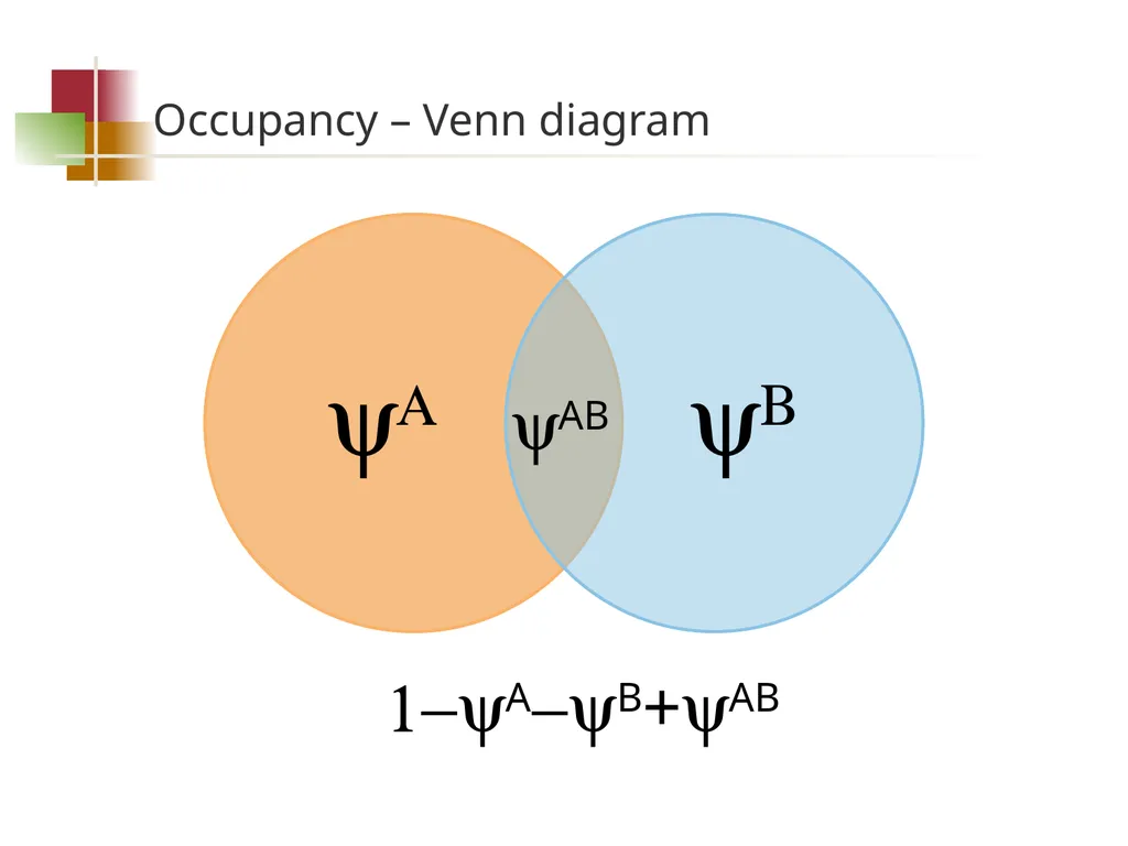
Occupancy – Venn diagram yAB 1-yA-yB+yAB<br>
08
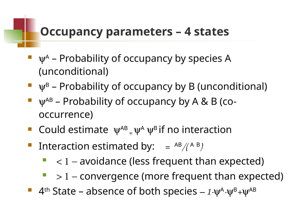
Occupancy parameters – 4 states yA – Probability of occupancy by species A (unconditional)
yB – Probability of occupancy by B (unconditional)
yAB – Probability of occupancy by A & B (co-occurrence)
Could estimate yAB = yA yB if no interaction
Interaction estimated by: = AB/(AB)
< 1 - avoidance (less frequent than expected)
> 1 - convergence (more frequent than expected)
4th State – absence of both species – 1-yA-yB+yAB<br>
09
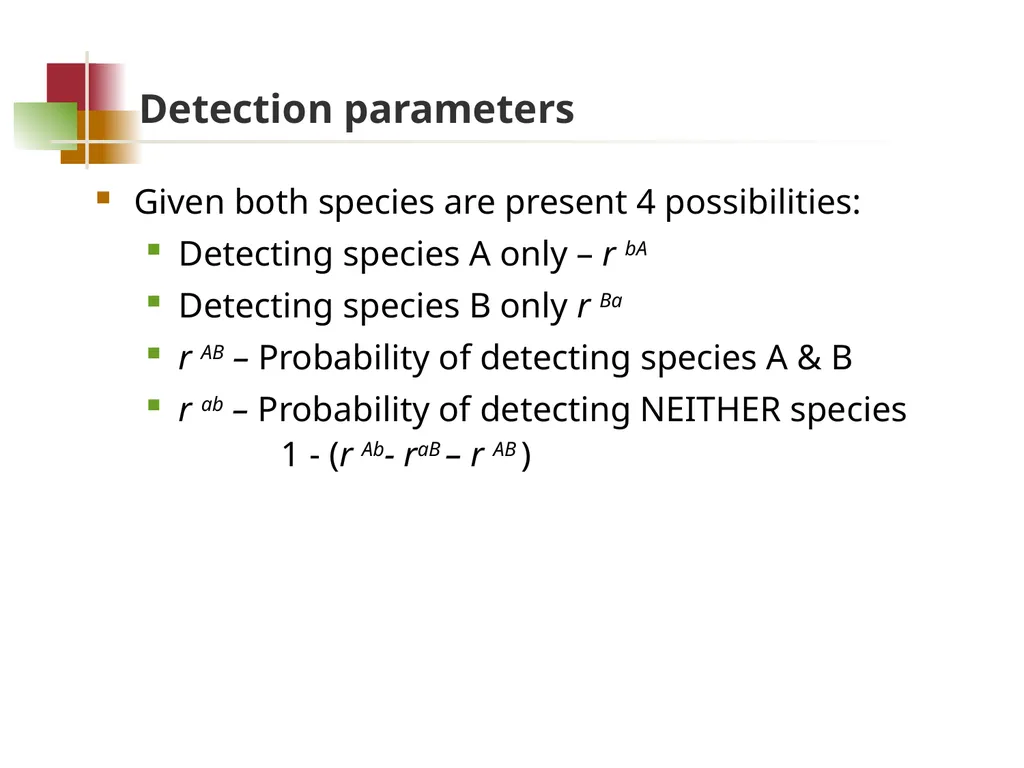
Detection parameters Given both species are present 4 possibilities:
Detecting species A only – r bA
Detecting species B only r Ba
r AB – Probability of detecting species A & B
r ab – Probability of detecting NEITHER species 1 - (r Ab- raB – r AB )<br>
10
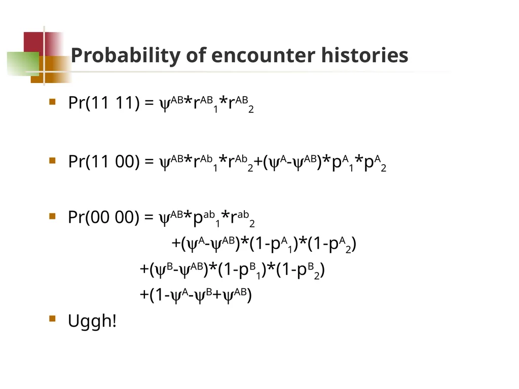
Probability of encounter histories Pr(11 11) = yAB*rAB1*rAB2
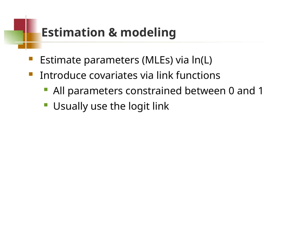
Estimation & modeling Estimate parameters (MLEs) via ln(L)
Introduce covariates via link functions
All parameters constrained between 0 and 1
Usually use the logit link<br>
12
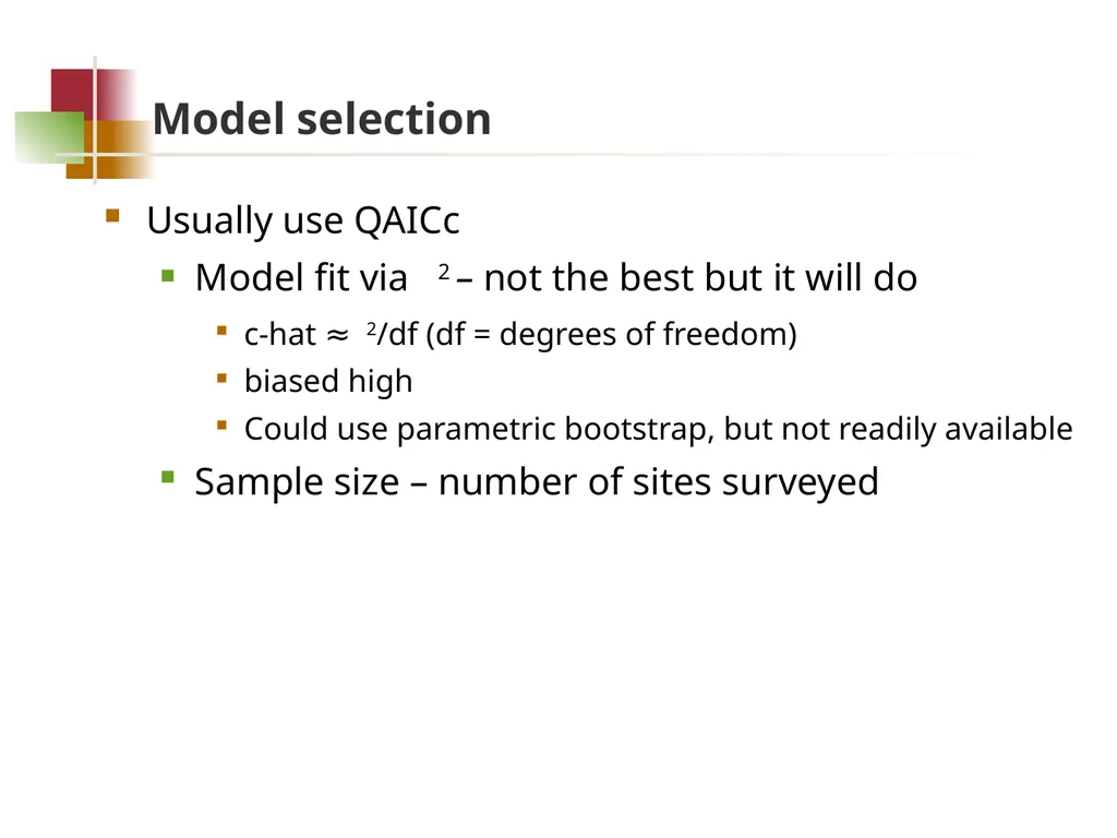
Model selection Usually use QAICc
Model fit via 2 – not the best but it will do
c-hat ≈ 2/df (df = degrees of freedom)
biased high
Could use parametric bootstrap, but not readily available
Sample size – number of sites surveyed<br>
13
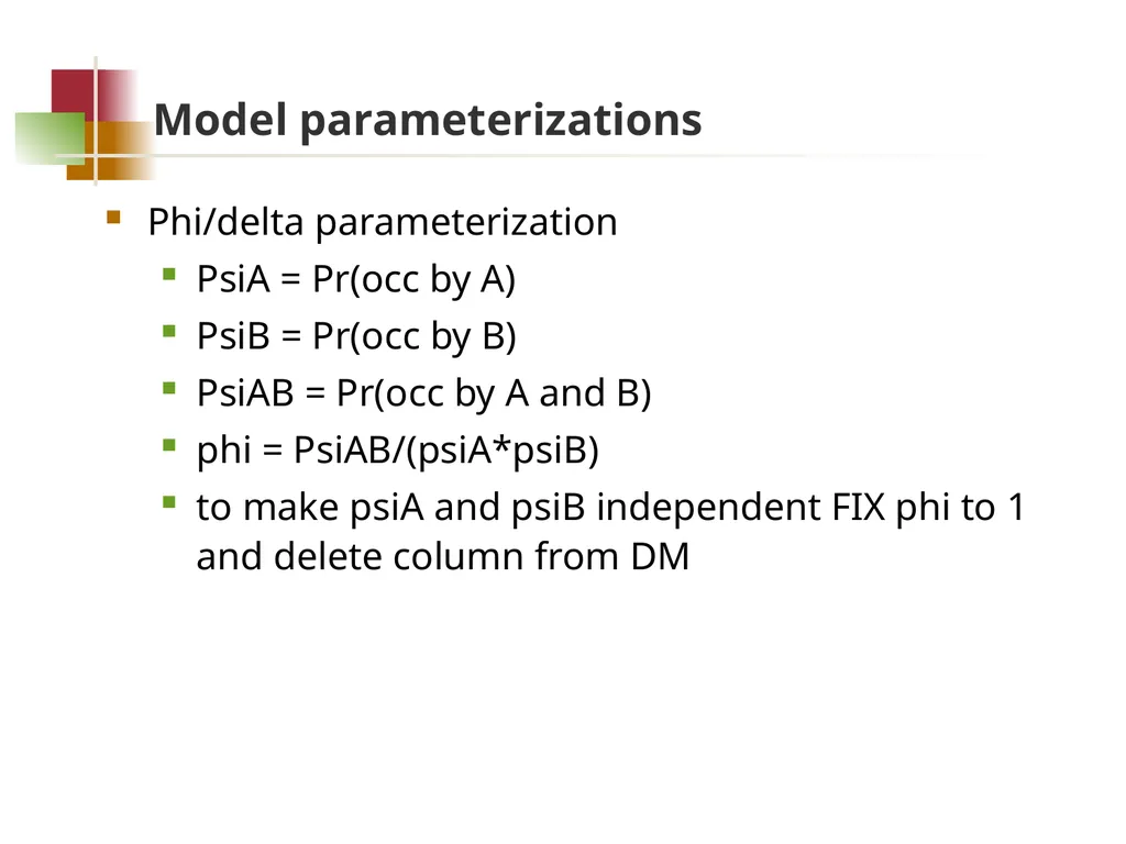
Model parameterizations Phi/delta parameterization
PsiA = Pr(occ by A)
PsiB = Pr(occ by B)
PsiAB = Pr(occ by A and B)
phi = PsiAB/(psiA*psiB)
to make psiA and psiB independent FIX phi to 1 and delete column from DM<br>
14
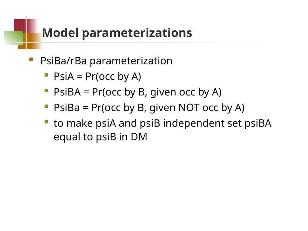
Model parameterizations PsiBa/rBa parameterization
PsiA = Pr(occ by A)
PsiBA = Pr(occ by B, given occ by A)
PsiBa = Pr(occ by B, given NOT occ by A)
to make psiA and psiB independent set psiBA equal to psiB in DM<br>
15
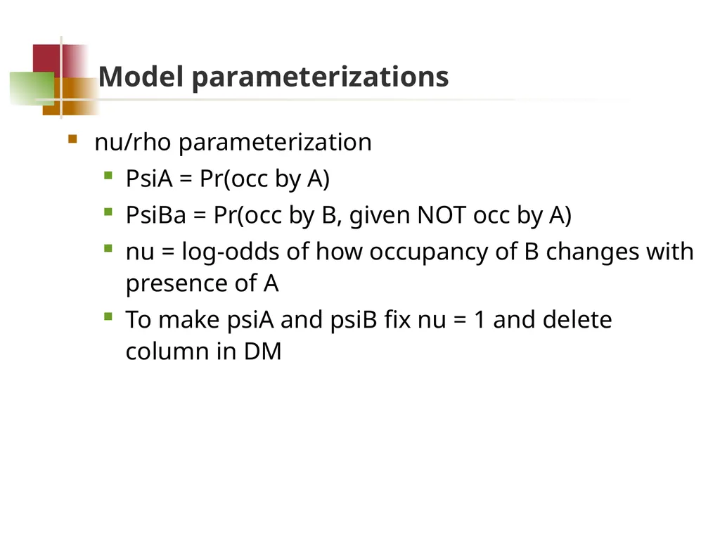
Model parameterizations nu/rho parameterization
PsiA = Pr(occ by A)
PsiBa = Pr(occ by B, given NOT occ by A)
nu = log-odds of how occupancy of B changes with presence of A
To make psiA and psiB fix nu = 1 and delete column in DM<br>
16
Additional Occupancy models (most in Presence)<br>
17
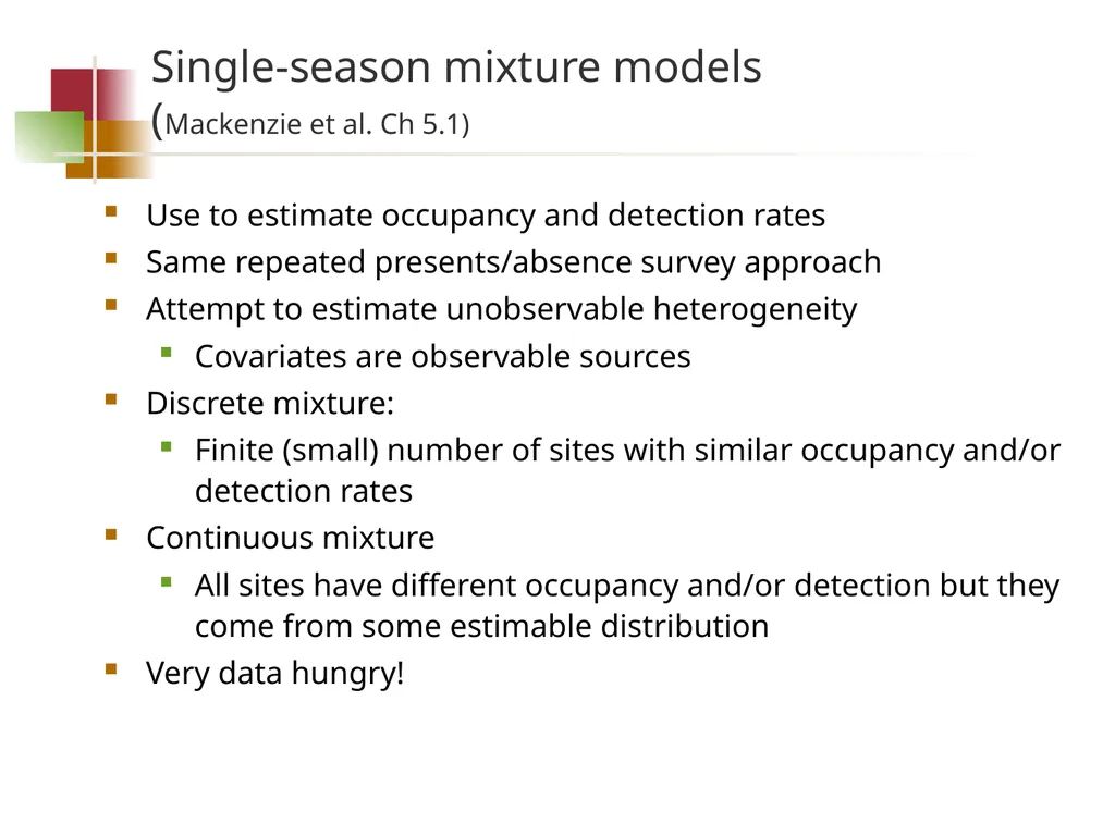
Single-season mixture models (Mackenzie et al. Ch 5.1) Use to estimate occupancy and detection rates
Same repeated presents/absence survey approach
Attempt to estimate unobservable heterogeneity
Covariates are observable sources
Discrete mixture:
Finite (small) number of sites with similar occupancy and/or detection rates
Continuous mixture
All sites have different occupancy and/or detection but they come from some estimable distribution
Very data hungry!<br>
18
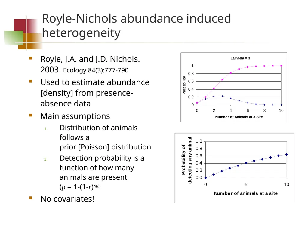
Royle-Nichols abundance induced heterogeneity Royle, J.A. and J.D. Nichols. 2003. Ecology 84(3):777-790
Used to estimate abundance [density] from presence-absence data
Main assumptions
Distribution of animals follows a prior [Poisson] distribution
Detection probability is a function of how many animals are present (p = 1-(1-r)N(i).
No covariates!<br>
19
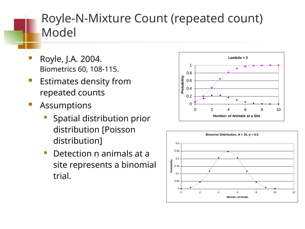
Royle-N-Mixture Count (repeated count) Model Royle, J.A. 2004. Biometrics 60, 108-115.
Estimates density from repeated counts
Assumptions
Spatial distribution prior distribution [Poisson distribution]
Detection n animals at a site represents a binomial trial.<br>
20
Single-season removal model Similar to single-season occupancy
Estimates occupancy and detection
Sites are no longer surveyed once species is detected
More efficient – allows more sites.
Assumptions:
Detection constant across surveys (not p(t))
Allows covariates but no site interactions<br>
21
Single-season multiple method Allows for different survey methods
Example large-scale and small-scale sampling
Assumption: if an individual is detected by one method, another is immediately available for detection by other method at that site.
Similar to robust design approach<br>
22
Species misidentification Royle, J. A., and W. Link. 2006. Ecology 87:835-841 Extends occupancy analysis to allow for false positives
Similar to mixture model
Some portion observations are false positives<br>
23
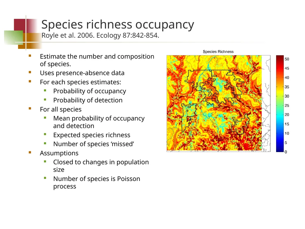
Species richness occupancy Royle et al. 2006. Ecology 87:842-854. Estimate the number and composition of species.
Uses presence-absence data
For each species estimates:
Probability of occupancy
Probability of detection
For all species
Mean probability of occupancy and detection
Expected species richness
Number of species ‘missed’
Assumptions
Closed to changes in population size
Number of species is Poisson process<br>
24
Multi-state occupancy Occupied sites are classified into multiple states
Estimates:
Occupancy, detection and probability of state
Assumption
Some state(s) can be identified with certainty
Example:
Breeding or non-breeding
Occupied-breeding-probable breeding<br>
25
Multi-season, multi-state occupancy Estimated parameters
Estimates occupancy given suitable initially
Probability that site is unsuitable in season
Detection given occupied
Extinction given suitable each season
Extinction given change from suitable to unsuitable
Colonization given change from unsuitable to suitable
Colonization given that suitable each season
Change from suitable to unsuitable
Change from unsuitable to suitable
Derived parameter
Remains suitable<br>
26
Occupancy with spatial correlation Hines et al. (in press) Estimates:
Occupancy
Detection
Spatial autocorrelation biases occupancy estimates<br>