State Space Search: Depth First Search Piyali

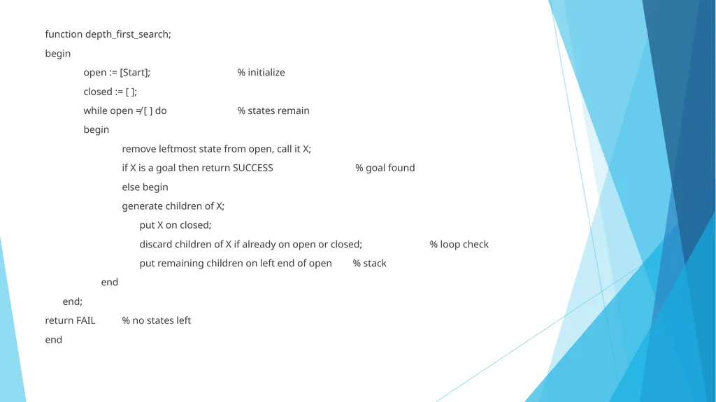
function depth_first_search;
begin
open := [Start]; % initialize
closed := [ ];
while open ≠ [ ] do % states remain
begin
remove leftmost state from open, call it X;
if X is a goal then return SUCCESS % goal found
else begin
generate children of X;
put X on closed;
discard children of X if already on open or closed; % loop check
put remaining children on left end of open % stack
end
end;
return FAIL % no states left
end<br>

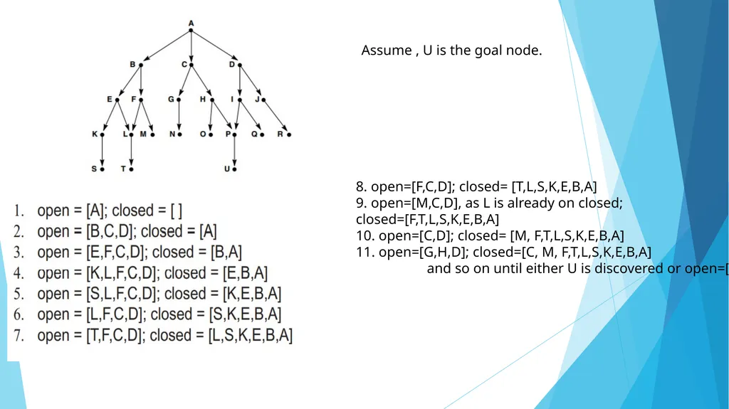
Assume , U is the goal node. 8. open=[F,C,D]; closed= [T,L,S,K,E,B,A]
9. open=[M,C,D], as L is already on closed; closed=[F,T,L,S,K,E,B,A]
10. open=[C,D]; closed= [M, F,T,L,S,K,E,B,A]
11. open=[G,H,D]; closed=[C, M, F,T,L,S,K,E,B,A]
and so on until either U is discovered or open=[].<br>

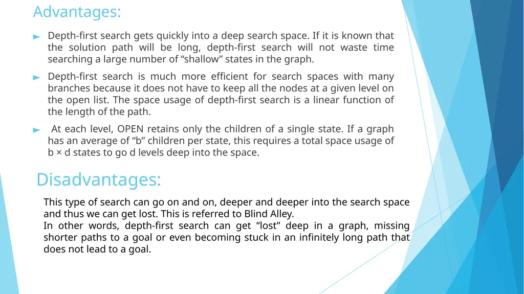
Advantages: Depth-first search gets quickly into a deep search space. If it is known that the solution path will be long, depth-first search will not waste time searching a large number of “shallow” states in the graph.
Depth-first search is much more efficient for search spaces with many branches because it does not have to keep all the nodes at a given level on the open list. The space usage of depth-first search is a linear function of the length of the path.
At each level, OPEN retains only the children of a single state. If a graph has an average of “b” children per state, this requires a total space usage of b × d states to go d levels deep into the space. Disadvantages: This type of search can go on and on, deeper and deeper into the search space and thus we can get lost. This is referred to Blind Alley.
In other words, depth-first search can get “lost” deep in a graph, missing shorter paths to a goal or even becoming stuck in an infinitely long path that does not lead to a goal.<br>

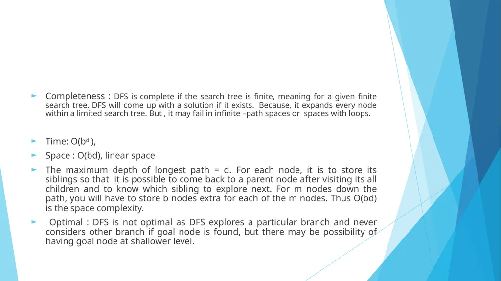
Completeness : DFS is complete if the search tree is finite, meaning for a given finite search tree, DFS will come up with a solution if it exists.  Because, it expands every node within a limited search tree. But , it may fail in infinite –path spaces or spaces with loops.

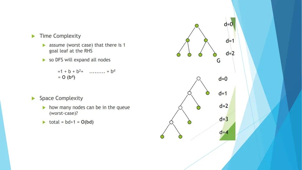
Time: O(bd ),
Space : O(bd), linear space
The maximum depth of longest path = d. For each node, it is to store its siblings so that it is possible to come back to a parent node after visiting its all children and to know which sibling to explore next. For m nodes down the path, you will have to store b nodes extra for each of the m nodes. Thus O(bd) is the space complexity.
Optimal : DFS is not optimal as DFS explores a particular branch and never considers other branch if goal node is found, but there may be possibility of having goal node at shallower level.<br>

BFS vs. DFS<br>

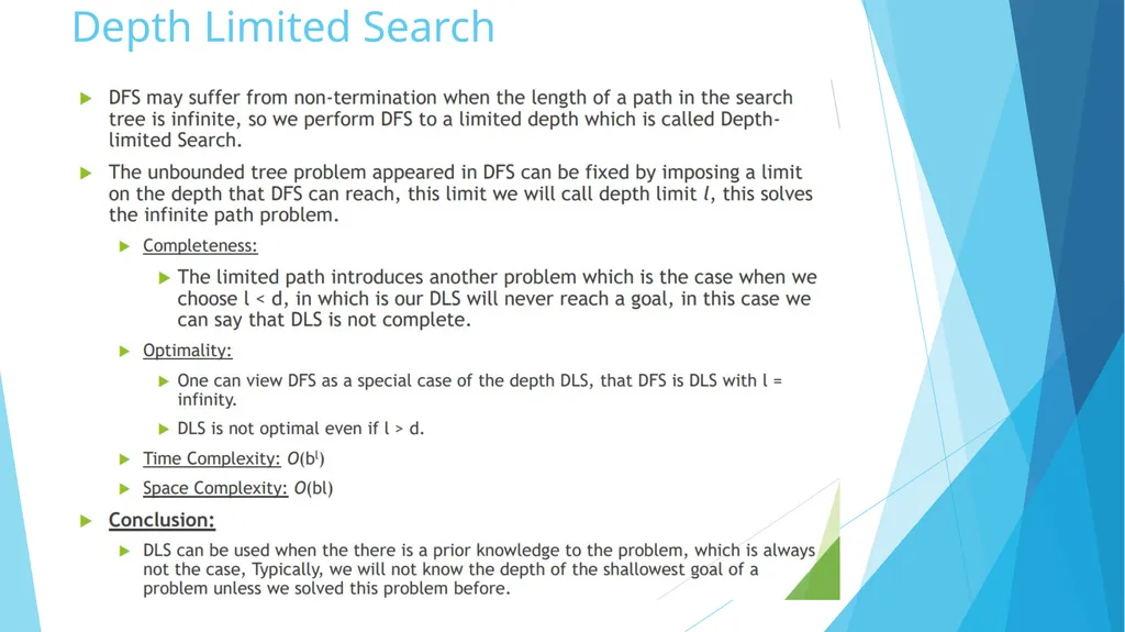
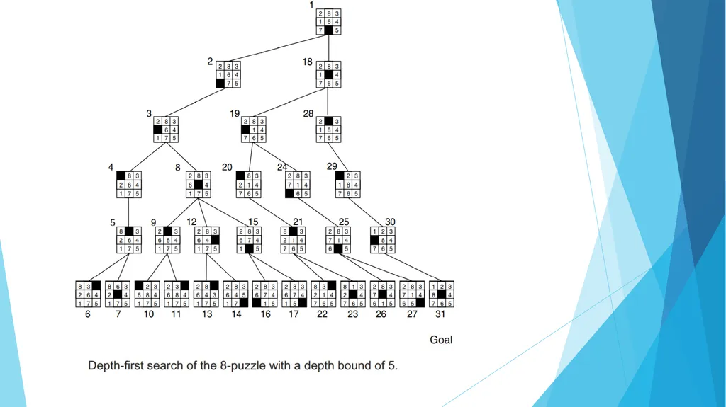
Depth Limited Search<br>

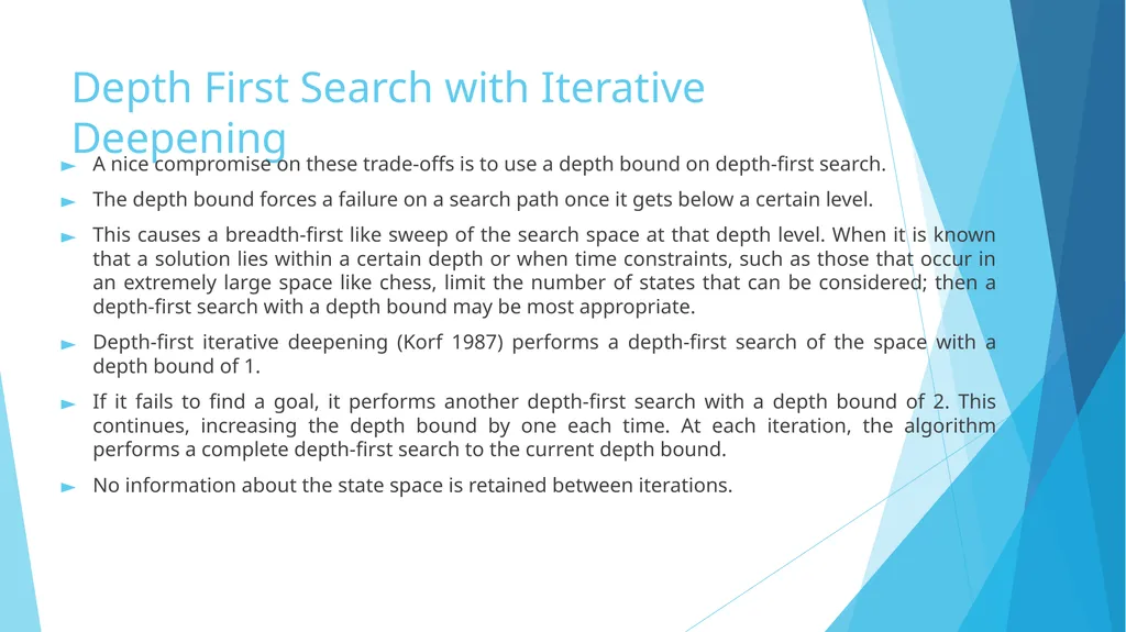
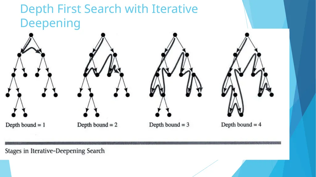
Depth First Search with Iterative Deepening A nice compromise on these trade-offs is to use a depth bound on depth-first search.
The depth bound forces a failure on a search path once it gets below a certain level.
This causes a breadth-first like sweep of the search space at that depth level. When it is known that a solution lies within a certain depth or when time constraints, such as those that occur in an extremely large space like chess, limit the number of states that can be considered; then a depth-first search with a depth bound may be most appropriate.
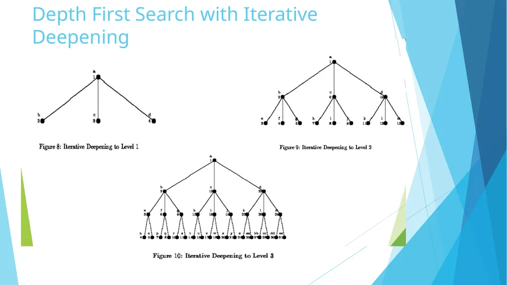
Depth-first iterative deepening (Korf 1987) performs a depth-first search of the space with a depth bound of 1.
If it fails to find a goal, it performs another depth-first search with a depth bound of 2. This continues, increasing the depth bound by one each time. At each iteration, the algorithm performs a complete depth-first search to the current depth bound.
No information about the state space is retained between iterations.<br>

Depth First Search with Iterative Deepening<br>

Depth First Search with Iterative Deepening<br>

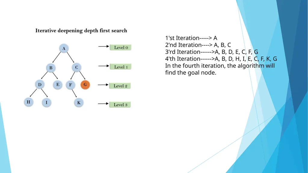
1'st Iteration-----> A2'nd Iteration----> A, B, C3'rd Iteration------>A, B, D, E, C, F, G4'th Iteration------>A, B, D, H, I, E, C, F, K, GIn the fourth iteration, the algorithm will find the goal node.<br>

Completeness:
This algorithm is complete is if the branching factor is finite.
Time Complexity:
If, b is the branching factor and depth is d then the worst-case time complexity is O(bd).

Space Complexity:
The space complexity of IDDFS will be O(bd).

Optimal:
This algorithm is optimal if path cost is a non- decreasing function of the depth of the node.<br>

Depth First Search with Iterative Deepening<br>

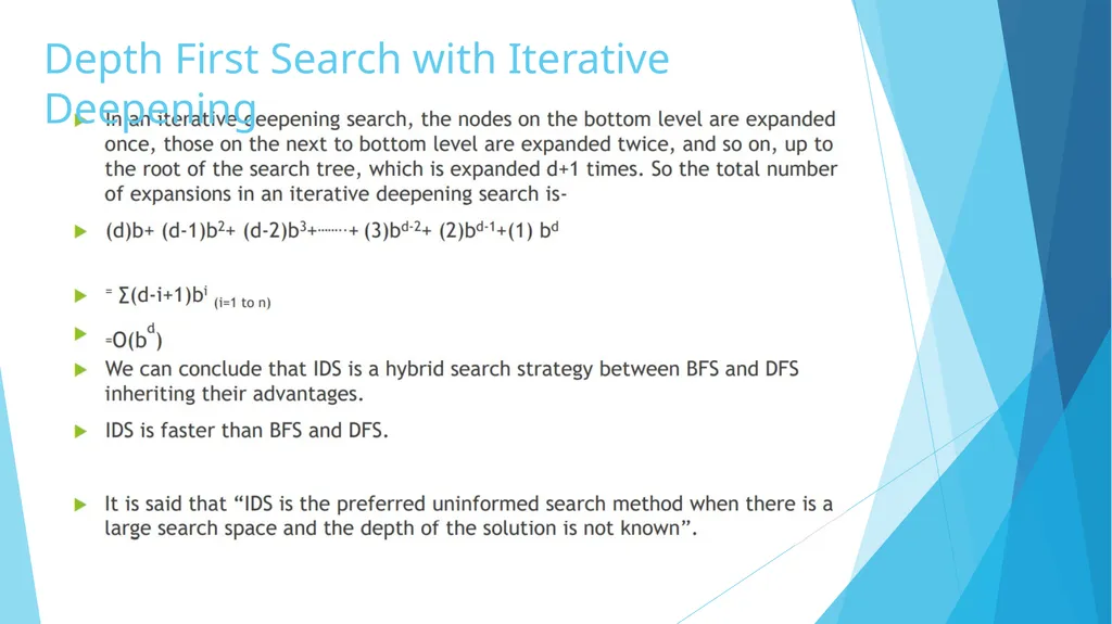
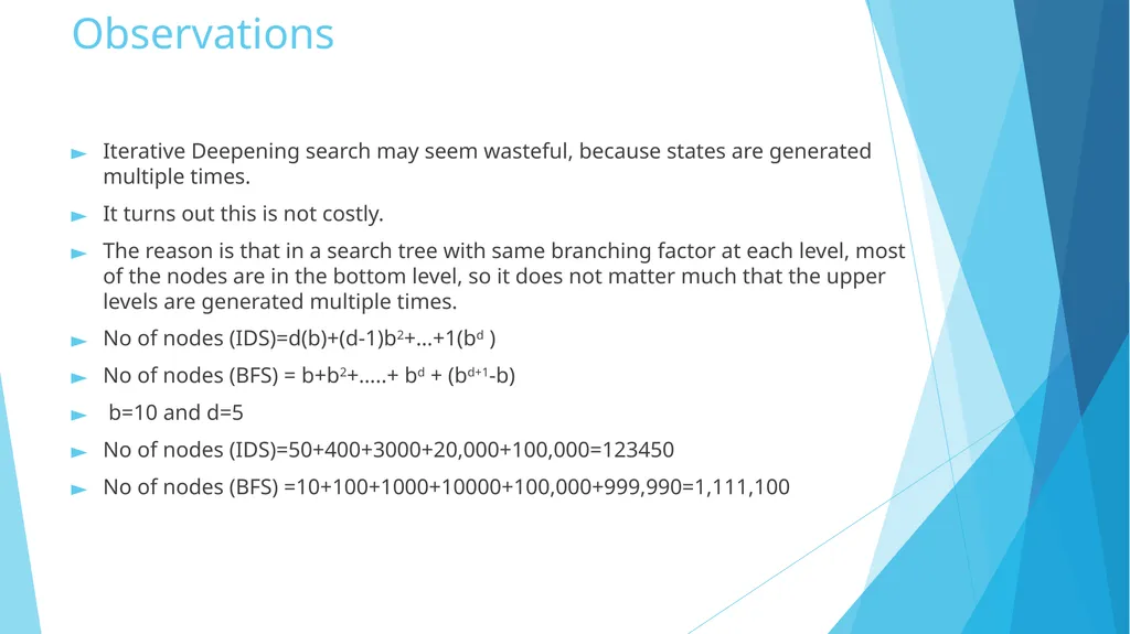
Observations Iterative Deepening search may seem wasteful, because states are generated multiple times.
It turns out this is not costly.
The reason is that in a search tree with same branching factor at each level, most of the nodes are in the bottom level, so it does not matter much that the upper levels are generated multiple times.
No of nodes (IDS)=d(b)+(d-1)b2+…+1(bd )
No of nodes (BFS) = b+b2+…..+ bd + (bd+1-b)
b=10 and d=5
No of nodes (IDS)=50+400+3000+20,000+100,000=123450
No of nodes (BFS) =10+100+1000+10000+100,000+999,990=1,111,100<br>

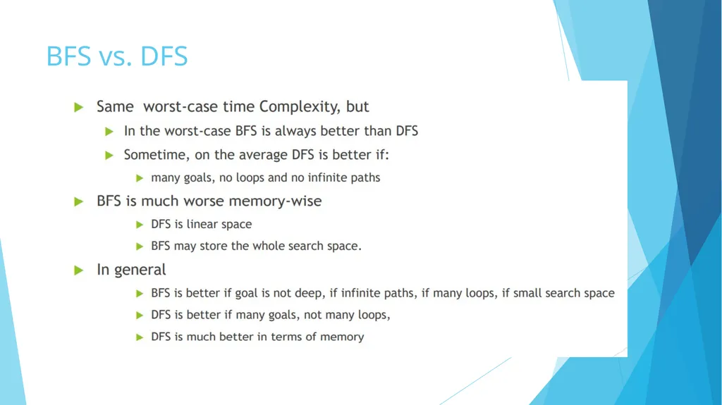
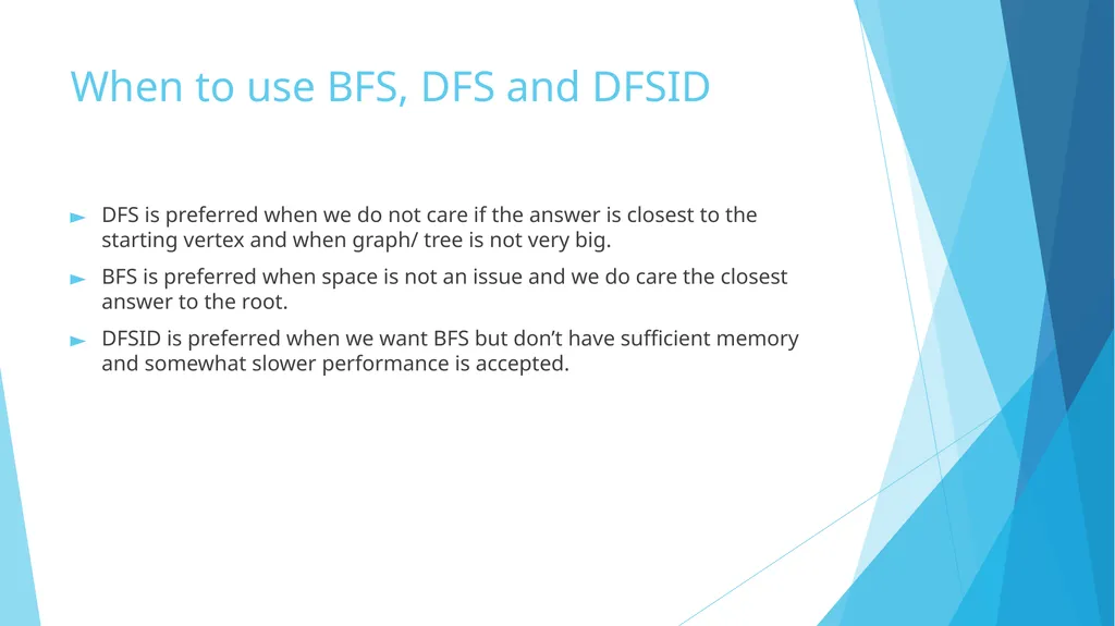
When to use BFS, DFS and DFSID DFS is preferred when we do not care if the answer is closest to the starting vertex and when graph/ tree is not very big.
BFS is preferred when space is not an issue and we do care the closest answer to the root.
DFSID is preferred when we want BFS but don’t have sufficient memory and somewhat slower performance is accepted.<br>