
Stats for Rats Statistical Considerations in Basic

Description: Stats for Rats Statistical Considerations in Basic Science Research Courtney McCracken, M.S., PhD(c) Traci Leong, PhD May 1st, 2012 Overview Biostatistics Core Basic principles of experimental design Sample size and power considerations
Related Topics
Download Presentation
"Stats for Rats Statistical Considerations in Basic" is the property of its rightful owner. Permission is granted to download and print the materials on this website for personal, non-commercial use only, and to display it on your personal computer provided you do not modify the materials and that you retain all copyright notices contained in the materials. By downloading content from our website, you accept the terms of this agreement.
Presentation Transcript
slide1. Stats for Rats
Statistical Considerations in Basic Science Research Courtney McCracken, M.S., PhD(c)
Traci Leong, PhD
May 1st, 2012<br>
slide2. Overview Biostatistics Core
Basic principles of experimental design
Sample size and power considerations
Data management<br>
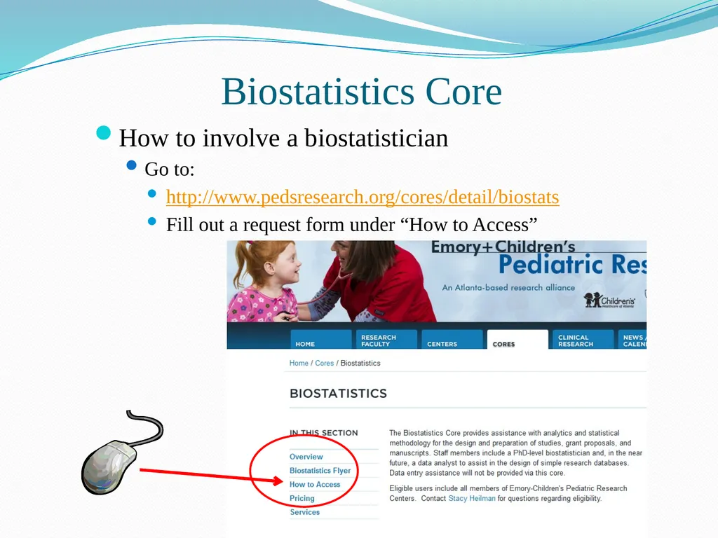
slide3. Biostatistics Core How to involve a biostatistician
Go to:
http://www.pedsresearch.org/cores/detail/biostats
Fill out a request form under “How to Access”<br>
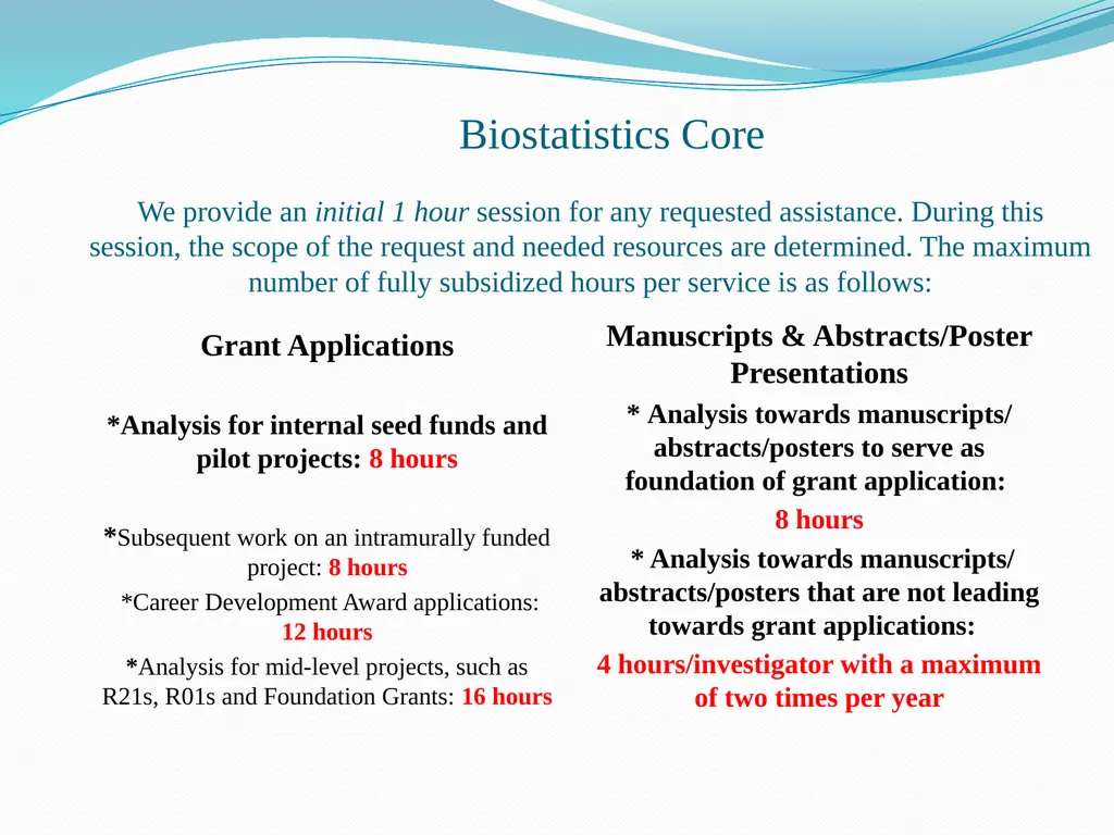
slide4. Biostatistics Core We provide an initial 1 hour session for any requested assistance. During this session, the scope of the request and needed resources are determined. The maximum number of fully subsidized hours per service is as follows: Grant Applications
*Analysis for internal seed funds and pilot projects: 8 hours
*Subsequent work on an intramurally funded project: 8 hours
*Career Development Award applications: 12 hours
*Analysis for mid-level projects, such as R21s, R01s and Foundation Grants: 16 hours Manuscripts & Abstracts/Poster Presentations
* Analysis towards manuscripts/ abstracts/posters to serve as foundation of grant application:
8 hours
* Analysis towards manuscripts/ abstracts/posters that are not leading towards grant applications:
4 hours/investigator with a maximum of two times per year<br>
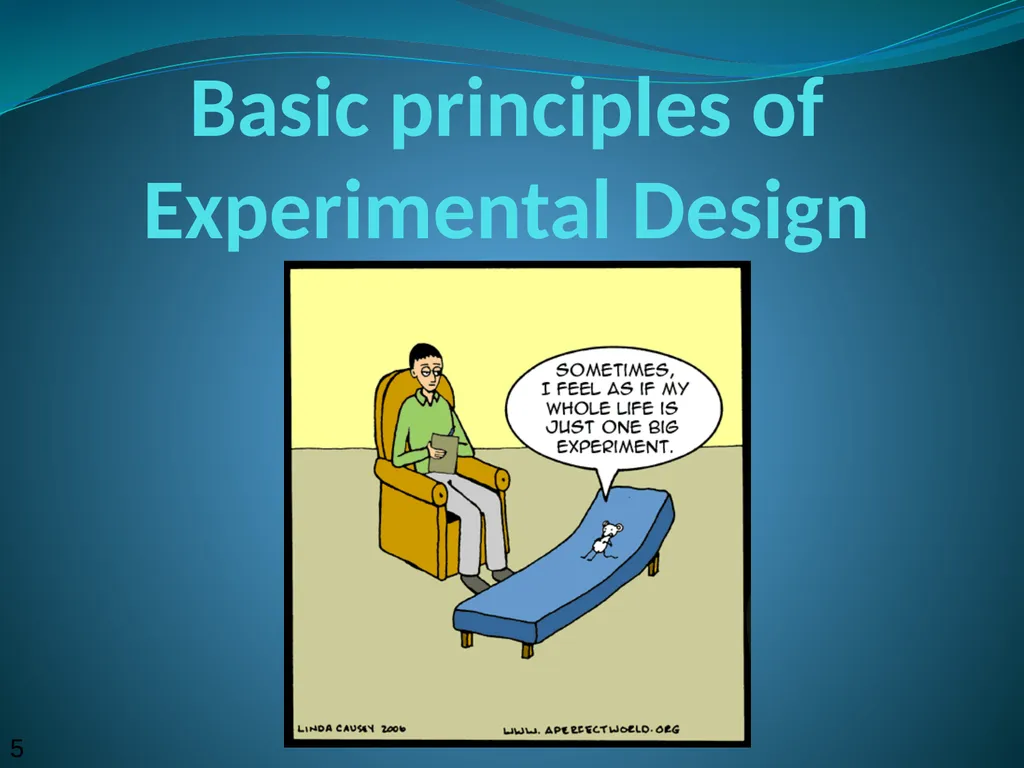
slide5. Basic principles of Experimental Design 5<br>
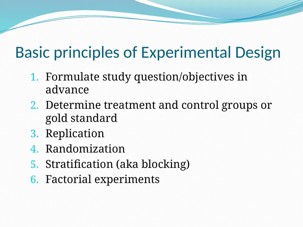
slide6. Basic principles of Experimental Design Formulate study question/objectives in advance
Determine treatment and control groups or gold standard
Replication
Randomization
Stratification (aka blocking)
Factorial experiments 6<br>
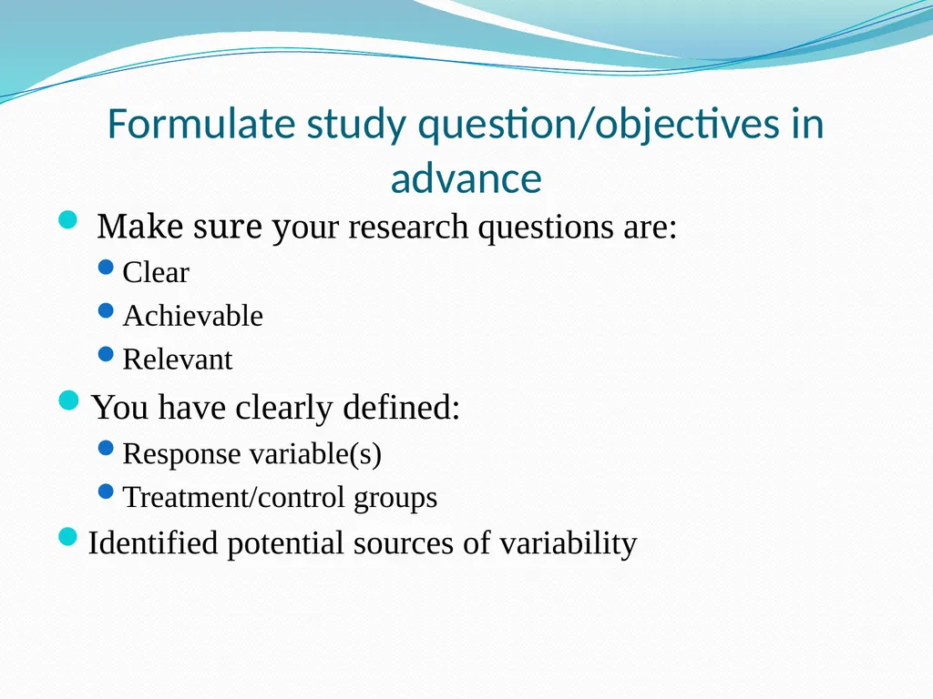
slide7. Formulate study question/objectives in advance Make sure your research questions are:
Clear
Achievable
Relevant
You have clearly defined:
Response variable(s)
Treatment/control groups
Identified potential sources of variability<br>
slide8. Multiple Response Variables
Many trials/experiments measure several outcomes
Must force investigator to rank them for importance
Do sample size on a few outcomes (2-3)
If estimates agree, OK…if not, must seek compromise Formulate study question/objectives in advance<br>
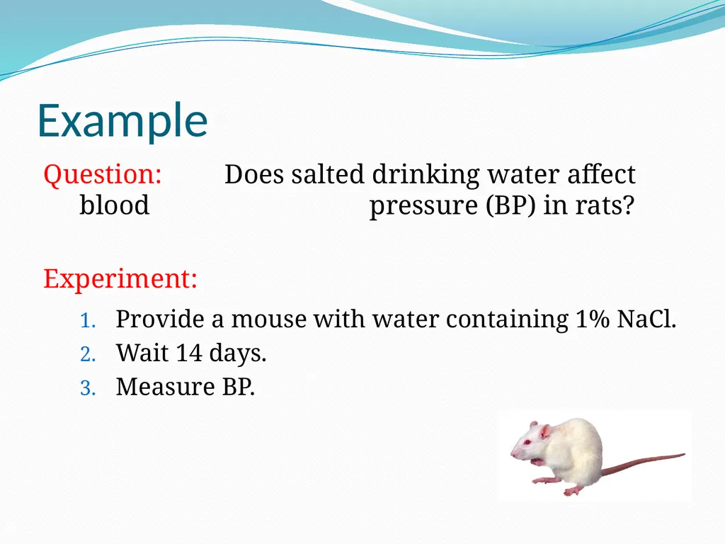
slide9. Example Question: Does salted drinking water affect blood pressure (BP) in rats?
Experiment:
Provide a mouse with water containing 1% NaCl.
Wait 14 days.
Measure BP. 9<br>
slide10. Comparison/control Good experiments are comparative.
Compare BP in rats fed salt water to BP in rats fed plain water.
Compare BP in strain A rats fed salt water to BP in strain B rats fed salt water.
Note: parallel controls are preferable over historical controls
Reduces variability 10<br>
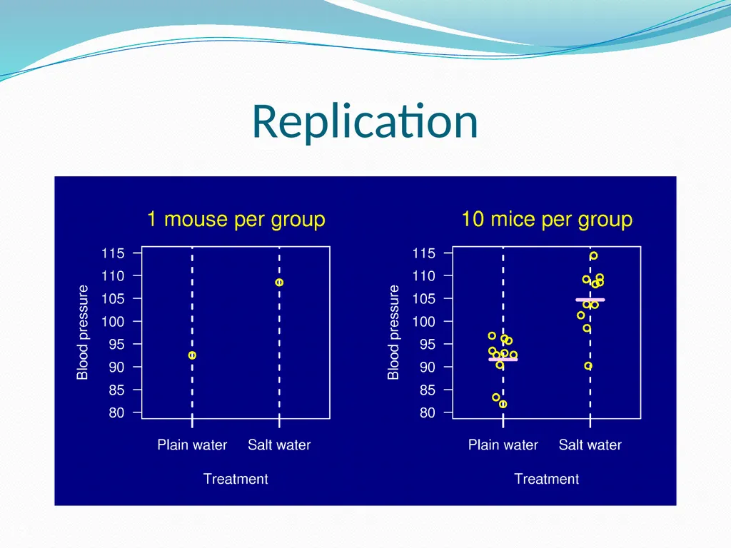
slide11. Replication Performing same experiment under identical conditions
Crucial in laboratory experiments
Reduce the effect of uncontrolled variation
Quantify uncertainty
To assure that results are reliable and valid
Replication can also introduce new sources of variability<br>
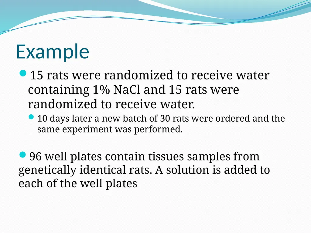
slide12. Example 15 rats were randomized to receive water containing 1% NaCl and 15 rats were randomized to receive water.
10 days later a new batch of 30 rats were ordered and the same experiment was performed.
96 well plates contain tissues samples from genetically identical rats. A solution is added to each of the well plates<br>
slide13. Replication 13<br>
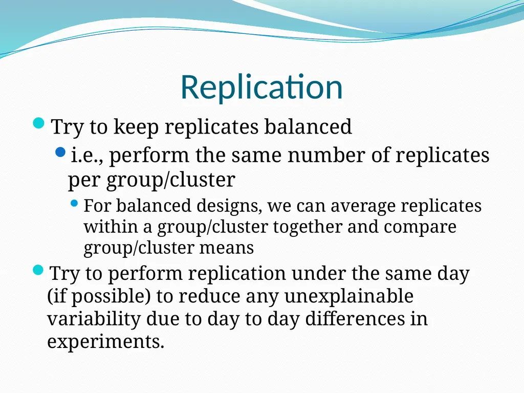
slide14. Replication Try to keep replicates balanced
i.e., perform the same number of replicates per group/cluster
For balanced designs, we can average replicates within a group/cluster together and compare group/cluster means
Try to perform replication under the same day (if possible) to reduce any unexplainable variability due to day to day differences in experiments.<br>
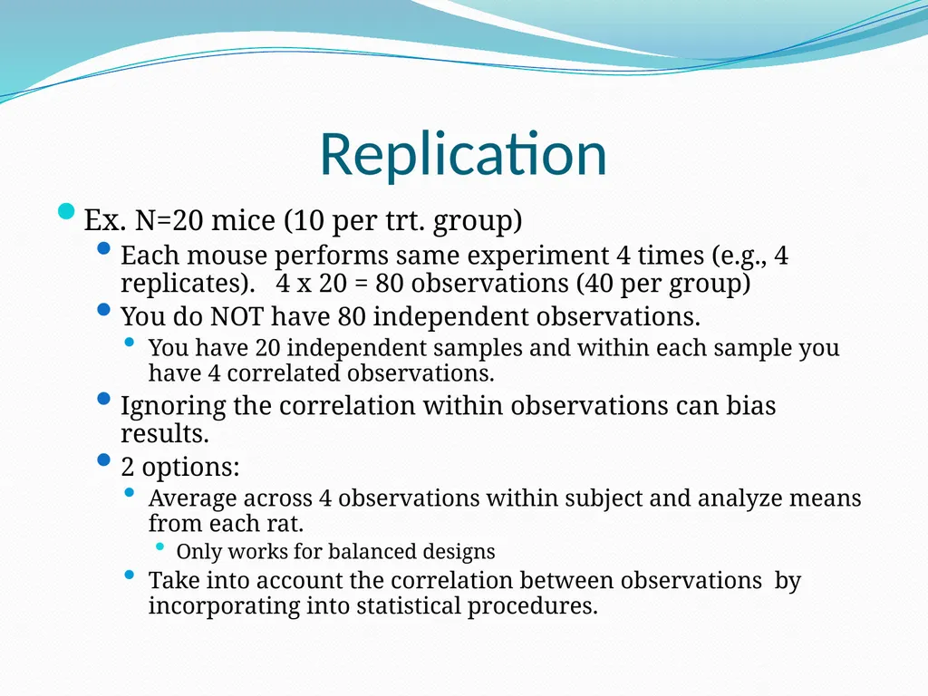
slide15. Replication Ex. N=20 mice (10 per trt. group)
Each mouse performs same experiment 4 times (e.g., 4 replicates). 4 x 20 = 80 observations (40 per group)
You do NOT have 80 independent observations.
You have 20 independent samples and within each sample you have 4 correlated observations.
Ignoring the correlation within observations can bias results.
2 options:
Average across 4 observations within subject and analyze means from each rat.
Only works for balanced designs
Take into account the correlation between observations by incorporating into statistical procedures.<br>
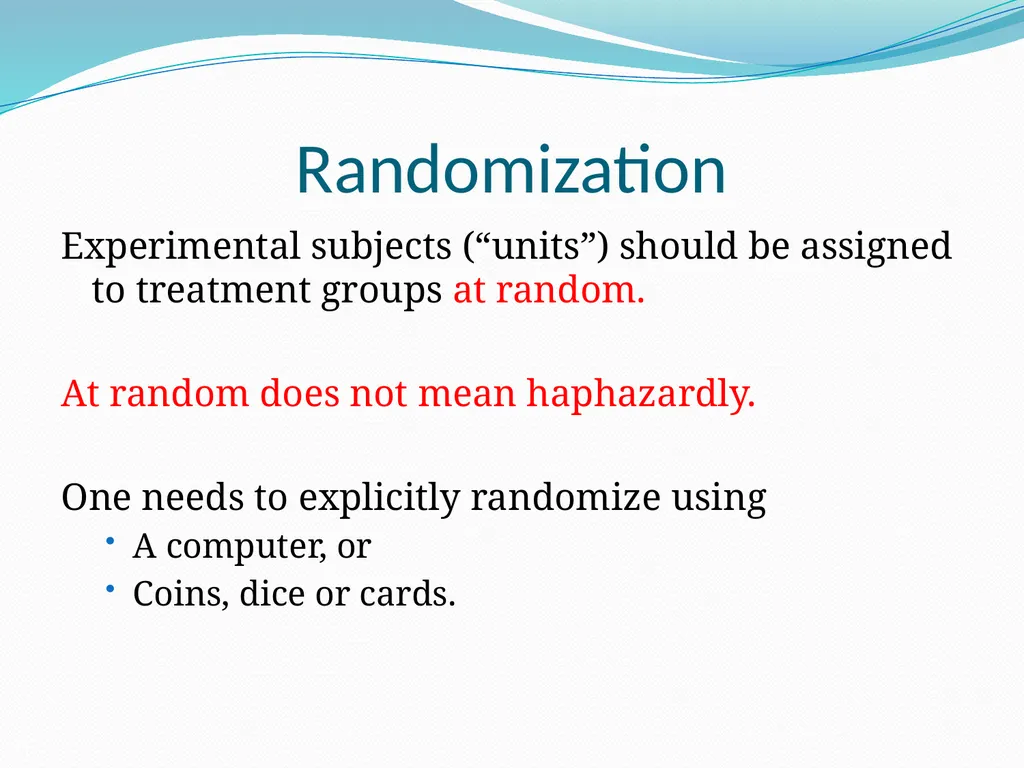
slide16. Randomization Experimental subjects (“units”) should be assigned to treatment groups at random.
At random does not mean haphazardly.
One needs to explicitly randomize using
A computer, or
Coins, dice or cards. 16<br>
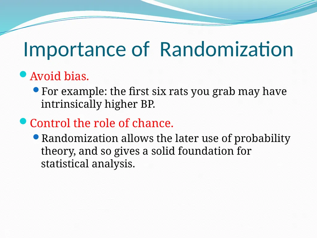
slide17. Importance of Randomization Avoid bias.
For example: the first six rats you grab may have intrinsically higher BP.
Control the role of chance.
Randomization allows the later use of probability theory, and so gives a solid foundation for statistical analysis. 17<br>
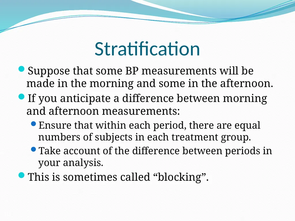
slide18. Stratification Suppose that some BP measurements will be made in the morning and some in the afternoon.
If you anticipate a difference between morning and afternoon measurements:
Ensure that within each period, there are equal numbers of subjects in each treatment group.
Take account of the difference between periods in your analysis.
This is sometimes called “blocking”. 18<br>
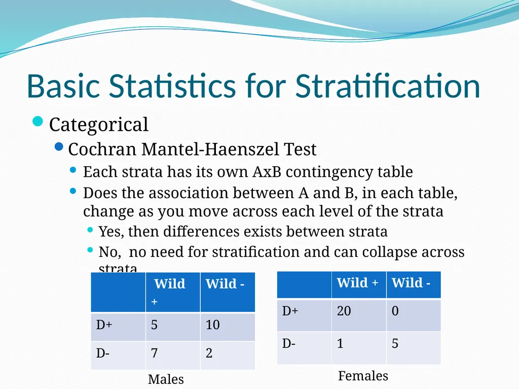
slide19. Basic Statistics for Stratification Categorical
Cochran Mantel-Haenszel Test
Each strata has its own AxB contingency table
Does the association between A and B, in each table, change as you move across each level of the strata
Yes, then differences exists between strata
No, no need for stratification and can collapse across strata Males Females<br>
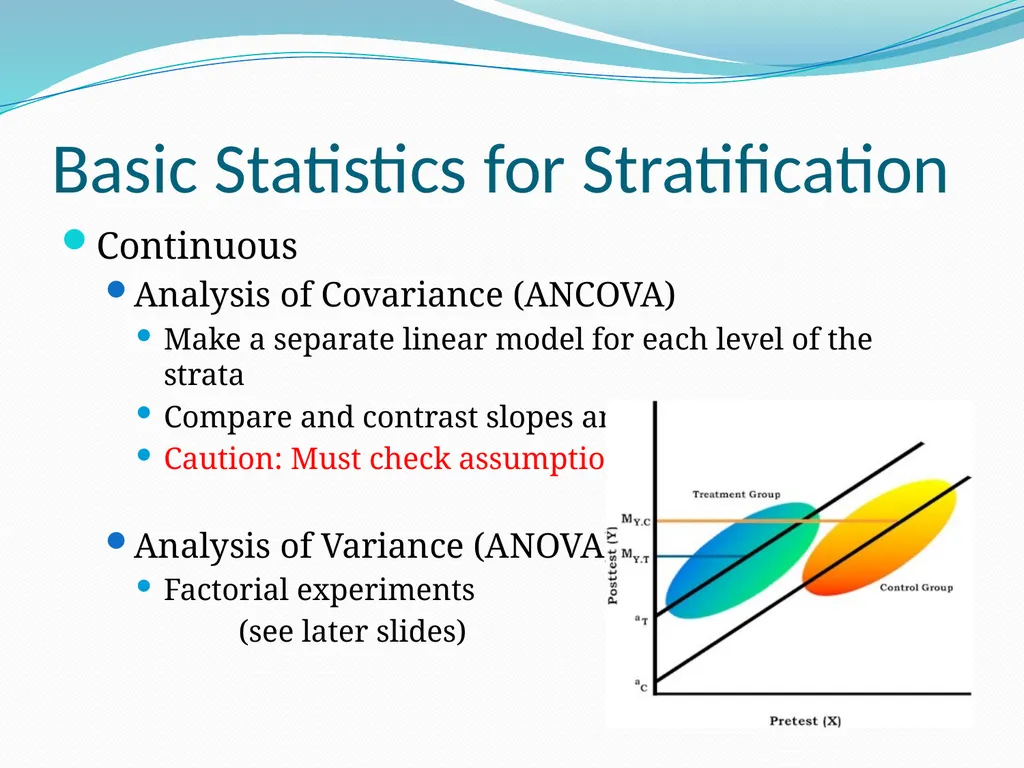
slide20. Basic Statistics for Stratification Continuous
Analysis of Covariance (ANCOVA)
Make a separate linear model for each level of the strata
Compare and contrast slopes and y-intercepts
Caution: Must check assumptions
Analysis of Variance (ANOVA)
Factorial experiments
(see later slides)<br>
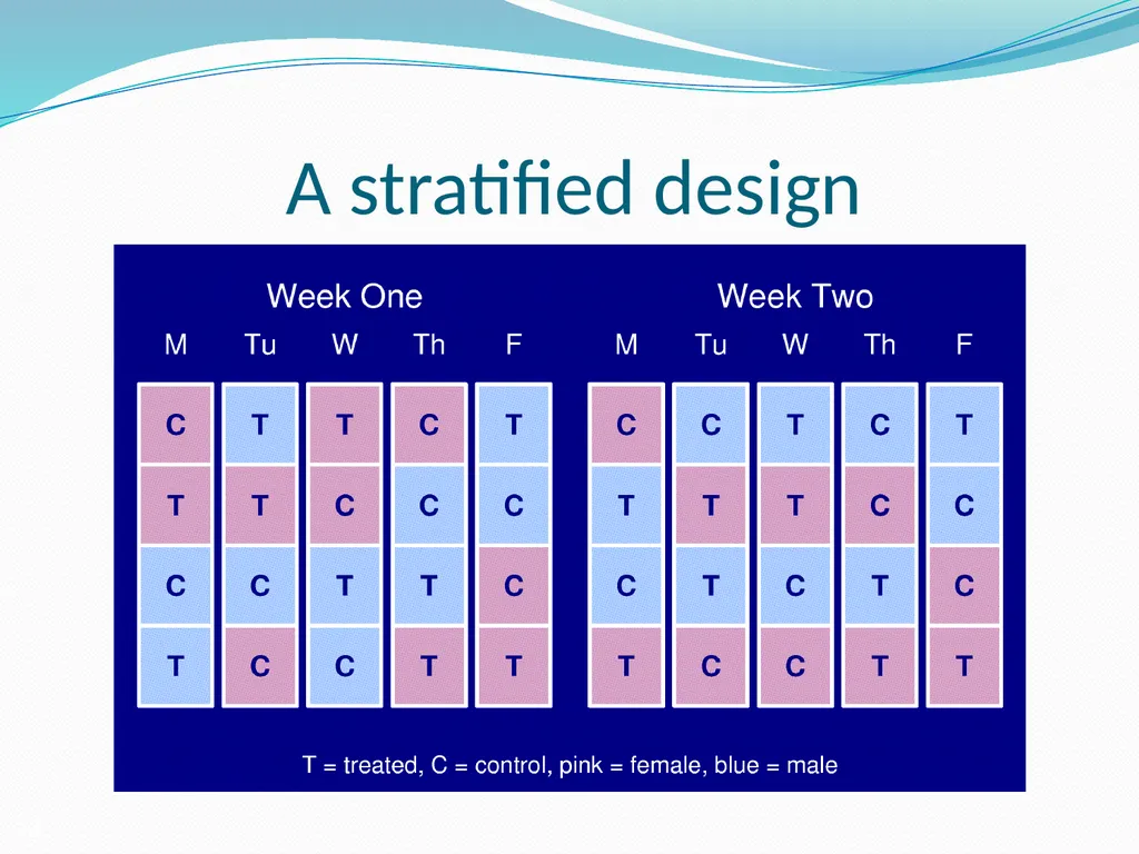
slide21. Example 20 male rats and 20 female rats.
Half to be treated; the other half left untreated.
Can only work with 4 rats per day.
Question? How to assign individuals to treatment
groups and to days? 21<br>
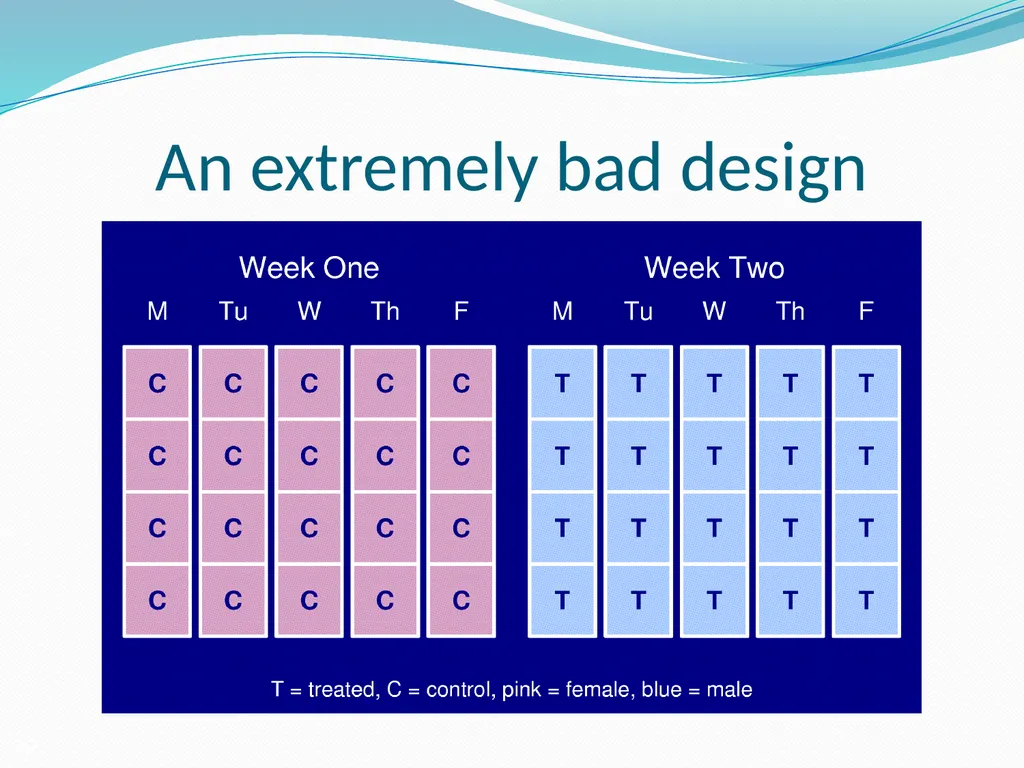
slide22. An extremely bad design 22<br>
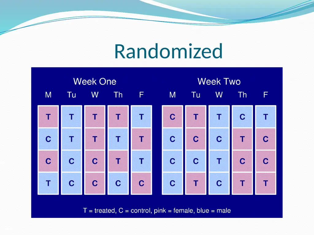
slide23. Randomized 23<br>
slide24. A stratified design 24<br>
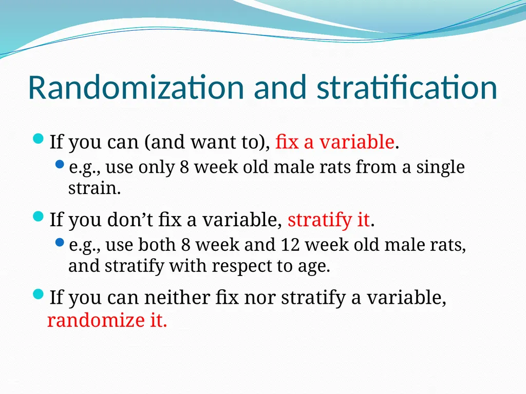
slide25. Randomization and stratification If you can (and want to), fix a variable.
e.g., use only 8 week old male rats from a single strain.
If you don’t fix a variable, stratify it.
e.g., use both 8 week and 12 week old male rats, and stratify with respect to age.
If you can neither fix nor stratify a variable, randomize it. 25<br>
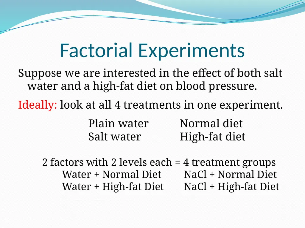
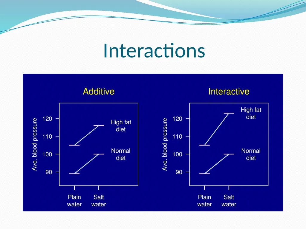
slide26. Factorial Experiments Suppose we are interested in the effect of both salt water and a high-fat diet on blood pressure.
Ideally: look at all 4 treatments in one experiment.
Plain water Normal diet
Salt water High-fat diet
2 factors with 2 levels each = 4 treatment groups
Water + Normal Diet NaCl + Normal Diet
Water + High-fat Diet NaCl + High-fat Diet 26<br>
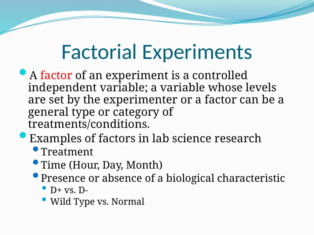
slide27. Factorial Experiments A factor of an experiment is a controlled independent variable; a variable whose levels are set by the experimenter or a factor can be a general type or category of treatments/conditions.
Examples of factors in lab science research
Treatment
Time (Hour, Day, Month)
Presence or absence of a biological characteristic
D+ vs. D-
Wild Type vs. Normal<br>
slide28. Factorial Experiments Adding additional factors leads to:
Increased sample size
Reduced Power
Possible interactions (good and unexplainable)
Additional complexity in modeling
Why do a factorial experiment?
We can learn more.
More efficient than doing all single-factor experiments.<br>
slide29. Interactions 29<br>
slide30. Statistics for Factorial Experiments ANOVA
One-Way
compare several groups of (independent) observations, test whether or not all the means are equal.
2 or more factors
Test for presences of interactions first
If significant report simple effects
condition on each factor at a time
If non-significant, remove from model and examine the main effects
Note: balanced designs are preferable, same n in every group.<br>
slide31. Repeated Factors If you are measuring the same subject repeatedly then observations are not independent
E.g., Measure BP at 1 hour, 2 hours, 4 hours after initiating treatment
We must account for correlation between observations
Try to only perform experiments with one-repeated factor.
Increasing the # of repeated factors significantly increases the sample size (have to model large correlation structures which require n<br>
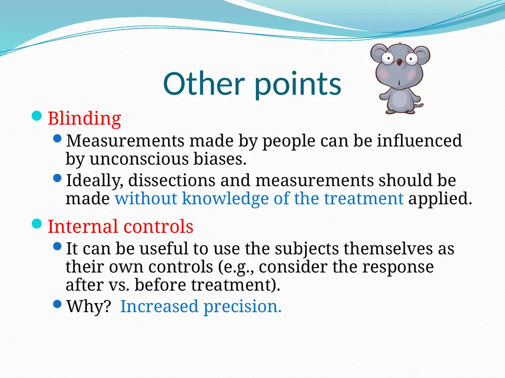
slide32. Other points Blinding
Measurements made by people can be influenced by unconscious biases.
Ideally, dissections and measurements should be made without knowledge of the treatment applied.
Internal controls
It can be useful to use the subjects themselves as their own controls (e.g., consider the response after vs. before treatment).
Why? Increased precision. 32<br>
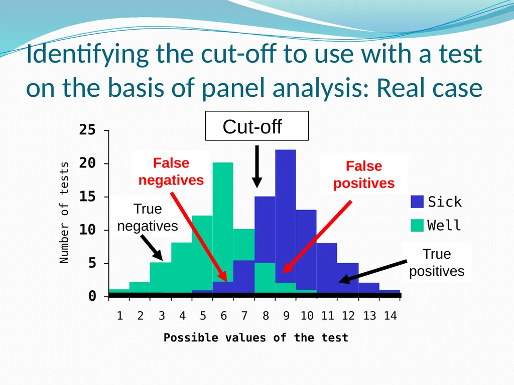
slide33. Identifying the cut-off to use with a test on the basis of panel analysis: Real case Cut-off 0 5 10 15 20 25 1 2 3 4 5 6 7 8 9 10 11 12 13 14 Possible values of the test Number of tests Sick Well<br>
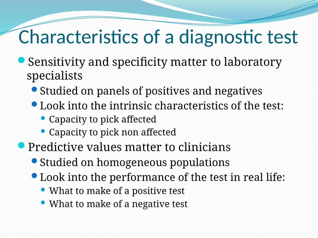
slide34. Characteristics of a diagnostic test Sensitivity and specificity matter to laboratory specialists
Studied on panels of positives and negatives
Look into the intrinsic characteristics of the test:
Capacity to pick affected
Capacity to pick non affected
Predictive values matter to clinicians
Studied on homogeneous populations
Look into the performance of the test in real life:
What to make of a positive test
What to make of a negative test<br>
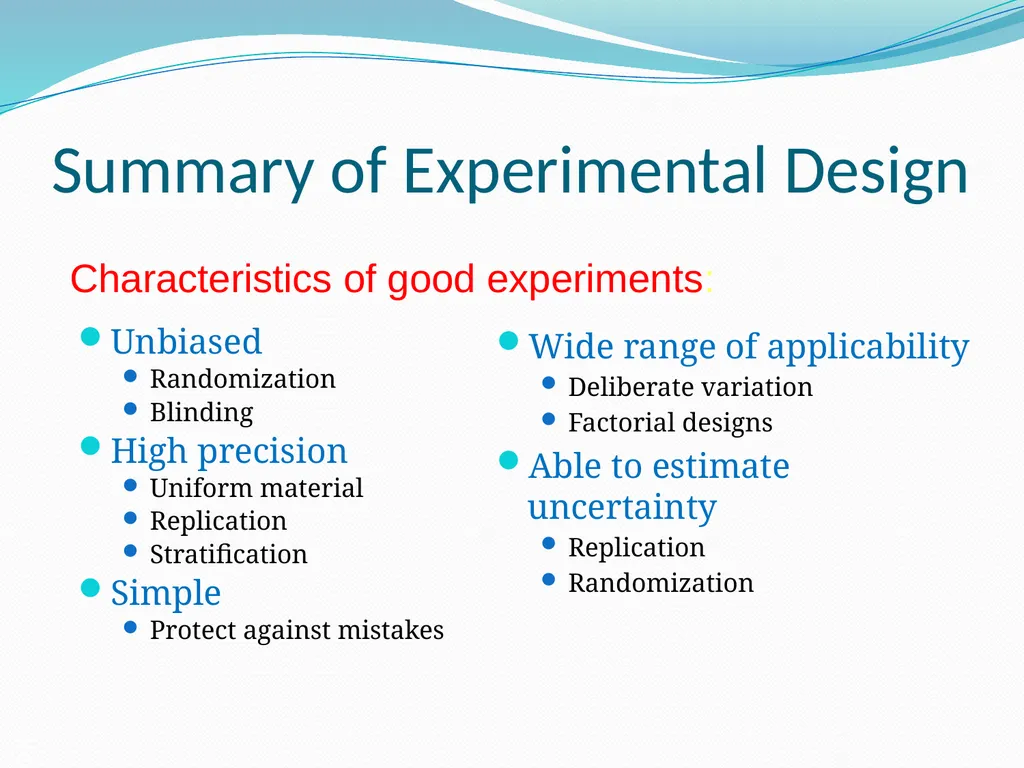
slide35. Summary of Experimental Design Unbiased
Randomization
Blinding
High precision
Uniform material
Replication
Stratification
Simple
Protect against mistakes Wide range of applicability
Deliberate variation
Factorial designs
Able to estimate uncertainty
Replication
Randomization Characteristics of good experiments: 35<br>
slide36. Sample size determination 36<br>
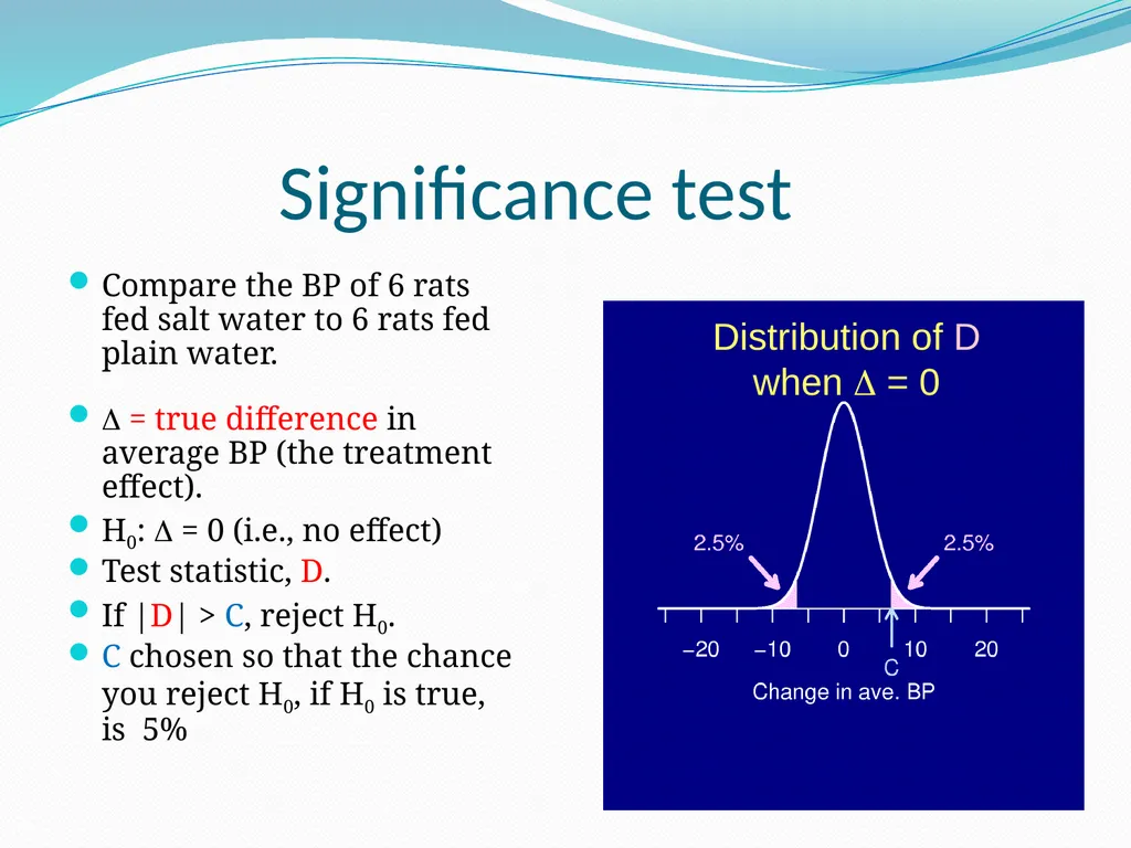
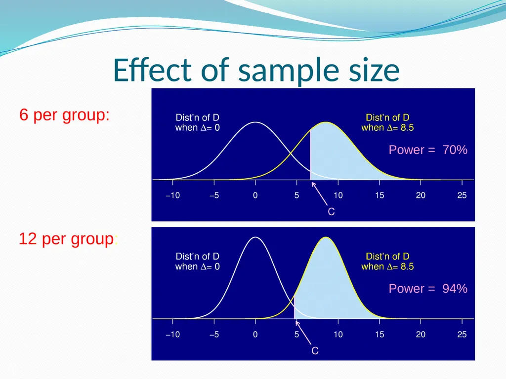
slide37. Significance test Compare the BP of 6 rats fed salt water to 6 rats fed plain water.
= true difference in average BP (the treatment effect).
H0: = 0 (i.e., no effect)
Test statistic, D.
If |D| > C, reject H0.
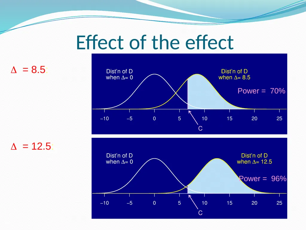
C chosen so that the chance you reject H0, if H0 is true, is 5% Distribution of D when = 0 37<br>
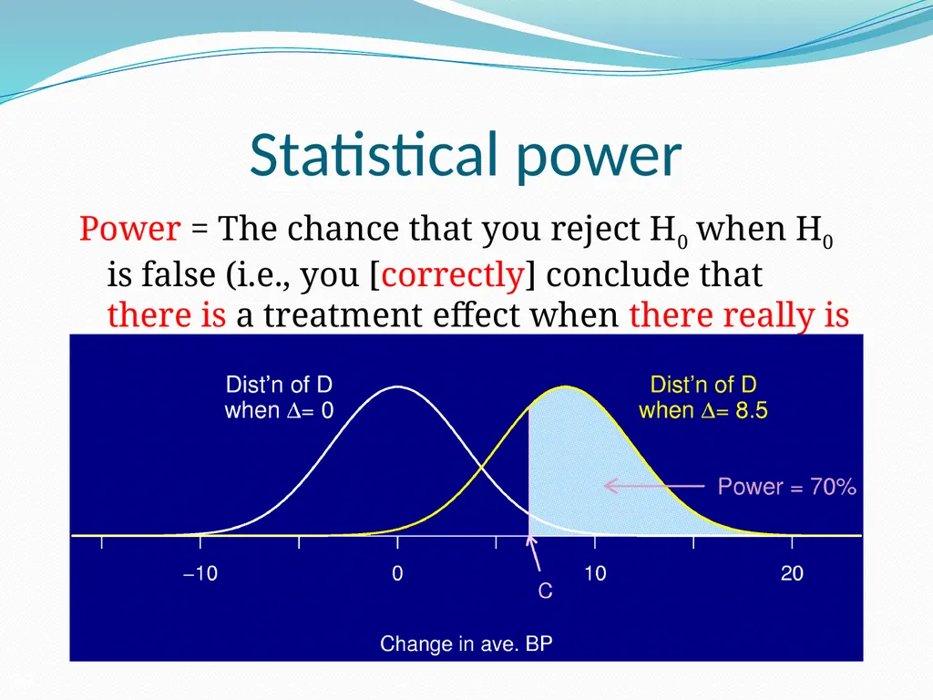
slide38. Statistical power Power = The chance that you reject H0 when H0 is false (i.e., you [correctly] conclude that there is a treatment effect when there really is a treatment effect). 38<br>
slide39. Power and sample size depend on… The design of the experiment
The method for analyzing the data (i.e., the statistical test)
The size of the true underlying effect
The variability in the measurements
The chosen significance level ()
The sample size 39<br>
slide40. Effect of sample size 6 per group: 12 per group: Power = 94% Power = 70% 40<br>
slide41. Effect of the effect = 8.5: = 12.5: Power = 70% Power = 96% 41<br>
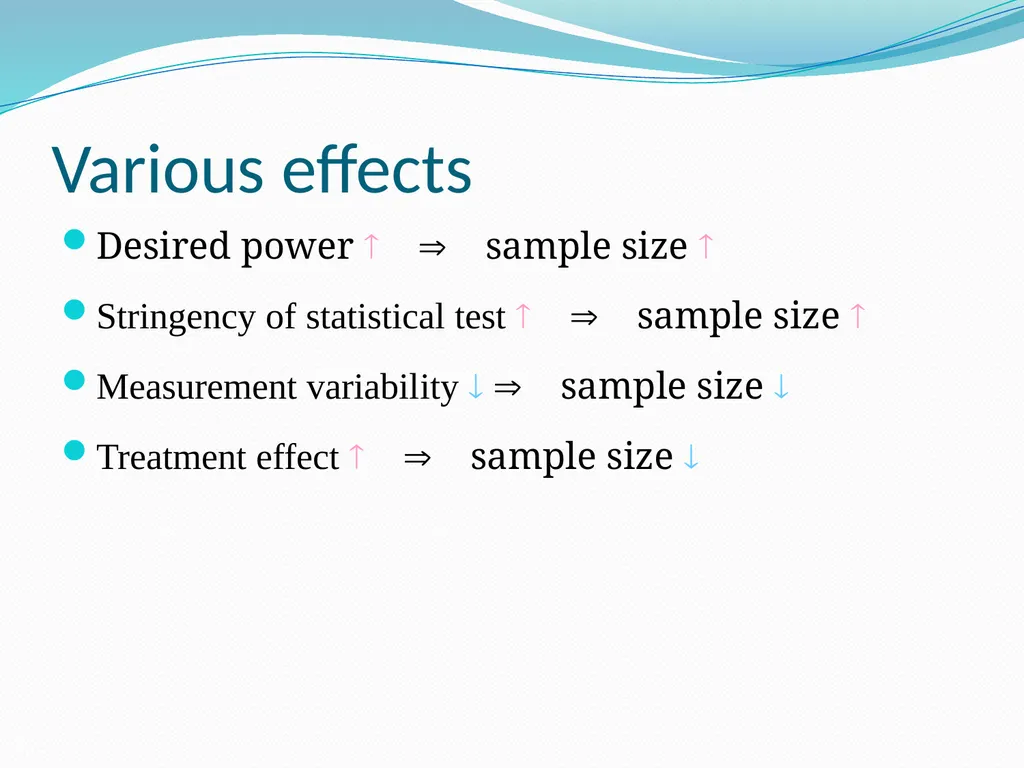
slide42. Various effects Desired power sample size
Stringency of statistical test sample size
Measurement variability sample size
Treatment effect sample size 42<br>
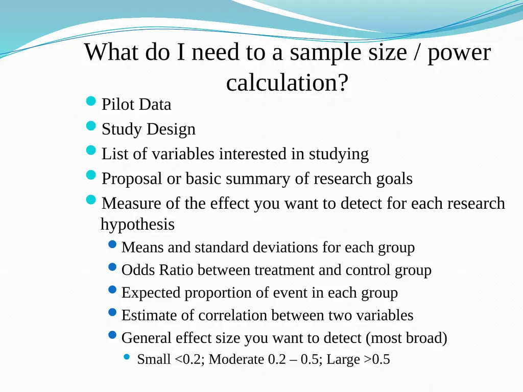
slide43. What do I need to a sample size / power calculation? Pilot Data
Study Design
List of variables interested in studying
Proposal or basic summary of research goals
Measure of the effect you want to detect for each research hypothesis
Means and standard deviations for each group
Odds Ratio between treatment and control group
Expected proportion of event in each group
Estimate of correlation between two variables
General effect size you want to detect (most broad)
Small <0.2; Moderate 0.2 – 0.5; Large >0.5<br>
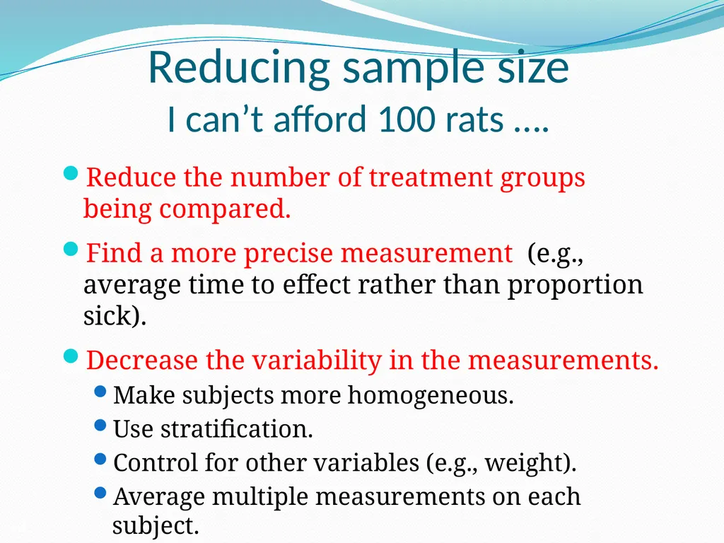
slide44. Reducing sample size I can’t afford 100 rats …. Reduce the number of treatment groups being compared.
Find a more precise measurement (e.g., average time to effect rather than proportion sick).
Decrease the variability in the measurements.
Make subjects more homogeneous.
Use stratification.
Control for other variables (e.g., weight).
Average multiple measurements on each subject. 44<br>
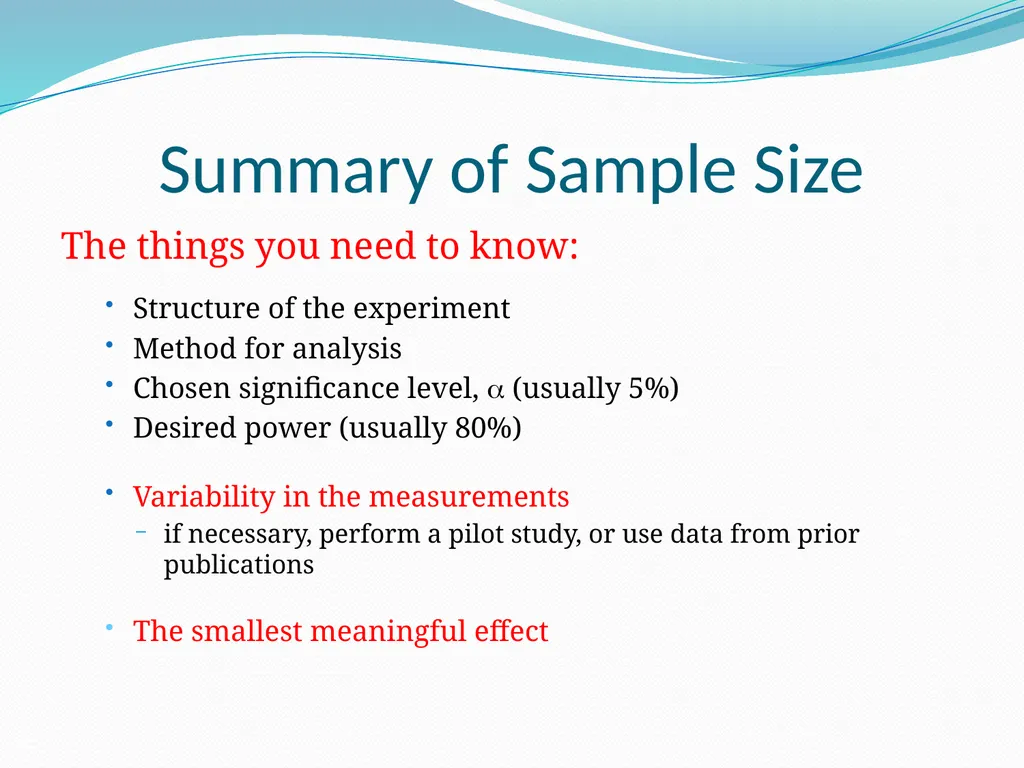
slide45. Summary of Sample Size The things you need to know:
Structure of the experiment
Method for analysis
Chosen significance level, (usually 5%)
Desired power (usually 80%)
Variability in the measurements
if necessary, perform a pilot study, or use data from prior publications
The smallest meaningful effect 45<br>
slide46. Data Management 46<br>
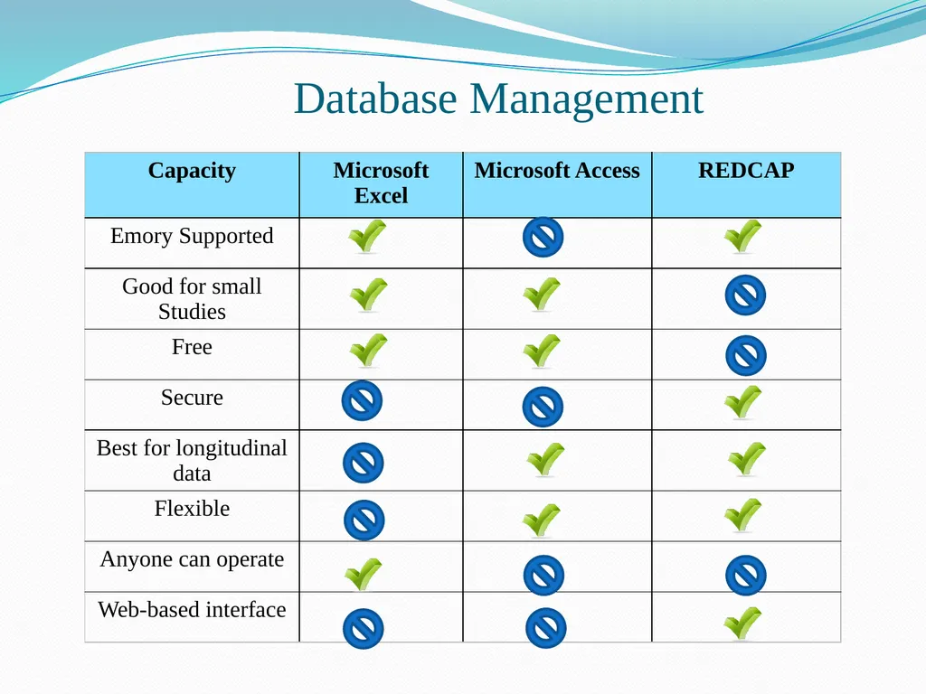
slide47. Database Management<br>
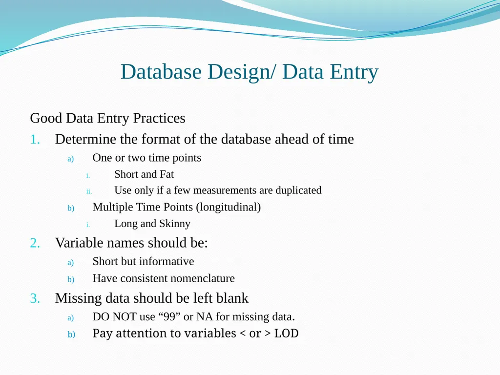
slide48. Database Design/ Data Entry Good Data Entry Practices
Determine the format of the database ahead of time
One or two time points
Short and Fat
Use only if a few measurements are duplicated
Multiple Time Points (longitudinal)
Long and Skinny
Variable names should be:
Short but informative
Have consistent nomenclature
Missing data should be left blank
DO NOT use “99” or NA for missing data.
Pay attention to variables < or > LOD<br>
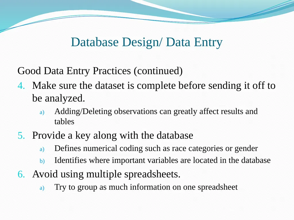
slide49. Good Data Entry Practices (continued)
Make sure the dataset is complete before sending it off to be analyzed.
Adding/Deleting observations can greatly affect results and tables
Provide a key along with the database
Defines numerical coding such as race categories or gender
Identifies where important variables are located in the database
Avoid using multiple spreadsheets.
Try to group as much information on one spreadsheet Database Design/ Data Entry<br>
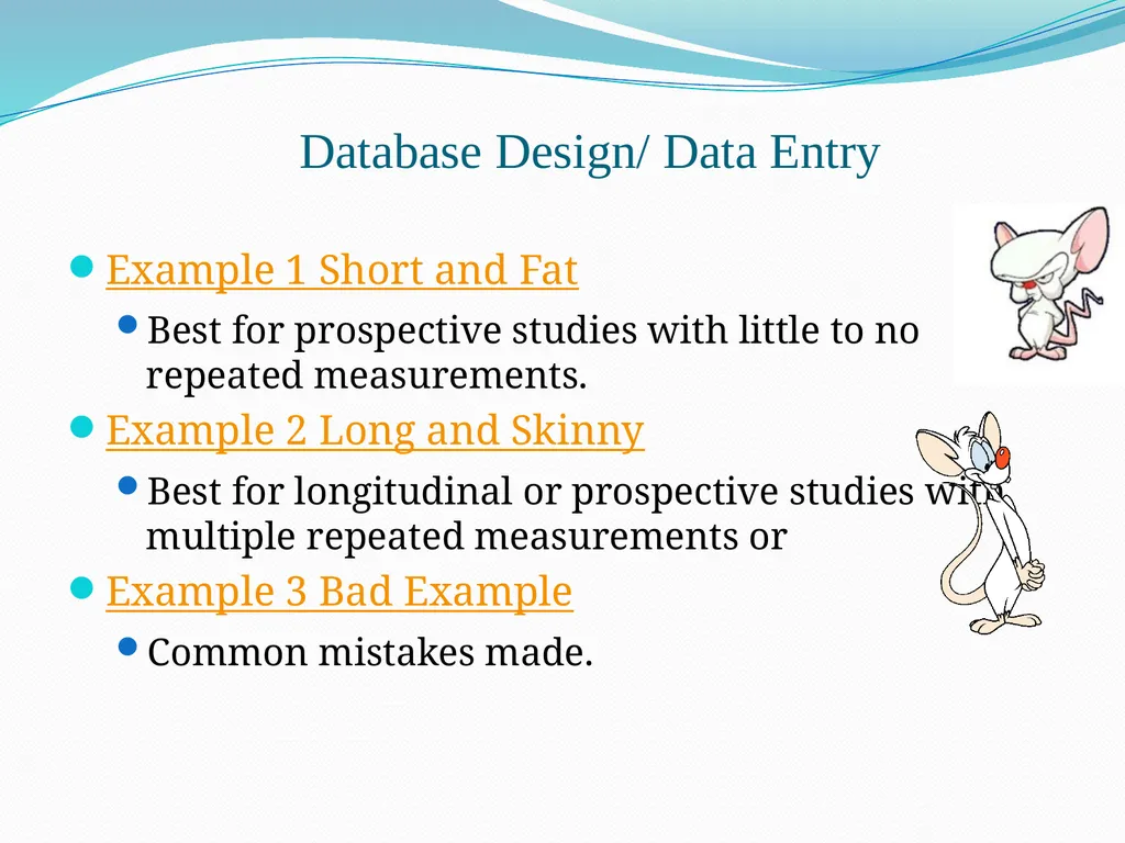
slide50. Example 1 Short and Fat
Best for prospective studies with little to no repeated measurements.
Example 2 Long and Skinny
Best for longitudinal or prospective studies with multiple repeated measurements or
Example 3 Bad Example
Common mistakes made. Database Design/ Data Entry<br>
slide51. Questions?<br>
slide52. Acknowledgement This presentation was adapted from Karl Broman’s lecture on Experimental Data.
This is part of a free lecture series from John Hopkins School of Public Health’s Open Courseware. For more information about additional lecture content from Dr. Broman please go to:
http://ocw.jhsph.edu/courses/StatisticsLaboratoryScientistsI/lectureNotes.cfm<br>
Traci Leong, PhD
May 1st, 2012<br>
slide2. Overview Biostatistics Core
Basic principles of experimental design
Sample size and power considerations
Data management<br>
slide3. Biostatistics Core How to involve a biostatistician
Go to:
http://www.pedsresearch.org/cores/detail/biostats
Fill out a request form under “How to Access”<br>
slide4. Biostatistics Core We provide an initial 1 hour session for any requested assistance. During this session, the scope of the request and needed resources are determined. The maximum number of fully subsidized hours per service is as follows: Grant Applications
*Analysis for internal seed funds and pilot projects: 8 hours
*Subsequent work on an intramurally funded project: 8 hours
*Career Development Award applications: 12 hours
*Analysis for mid-level projects, such as R21s, R01s and Foundation Grants: 16 hours Manuscripts & Abstracts/Poster Presentations
* Analysis towards manuscripts/ abstracts/posters to serve as foundation of grant application:
8 hours
* Analysis towards manuscripts/ abstracts/posters that are not leading towards grant applications:
4 hours/investigator with a maximum of two times per year<br>
slide5. Basic principles of Experimental Design 5<br>
slide6. Basic principles of Experimental Design Formulate study question/objectives in advance
Determine treatment and control groups or gold standard
Replication
Randomization
Stratification (aka blocking)
Factorial experiments 6<br>
slide7. Formulate study question/objectives in advance Make sure your research questions are:
Clear
Achievable
Relevant
You have clearly defined:
Response variable(s)
Treatment/control groups
Identified potential sources of variability<br>
slide8. Multiple Response Variables
Many trials/experiments measure several outcomes
Must force investigator to rank them for importance
Do sample size on a few outcomes (2-3)
If estimates agree, OK…if not, must seek compromise Formulate study question/objectives in advance<br>
slide9. Example Question: Does salted drinking water affect blood pressure (BP) in rats?
Experiment:
Provide a mouse with water containing 1% NaCl.
Wait 14 days.
Measure BP. 9<br>
slide10. Comparison/control Good experiments are comparative.
Compare BP in rats fed salt water to BP in rats fed plain water.
Compare BP in strain A rats fed salt water to BP in strain B rats fed salt water.
Note: parallel controls are preferable over historical controls
Reduces variability 10<br>
slide11. Replication Performing same experiment under identical conditions
Crucial in laboratory experiments
Reduce the effect of uncontrolled variation
Quantify uncertainty
To assure that results are reliable and valid
Replication can also introduce new sources of variability<br>
slide12. Example 15 rats were randomized to receive water containing 1% NaCl and 15 rats were randomized to receive water.
10 days later a new batch of 30 rats were ordered and the same experiment was performed.
96 well plates contain tissues samples from genetically identical rats. A solution is added to each of the well plates<br>
slide13. Replication 13<br>
slide14. Replication Try to keep replicates balanced
i.e., perform the same number of replicates per group/cluster
For balanced designs, we can average replicates within a group/cluster together and compare group/cluster means
Try to perform replication under the same day (if possible) to reduce any unexplainable variability due to day to day differences in experiments.<br>
slide15. Replication Ex. N=20 mice (10 per trt. group)
Each mouse performs same experiment 4 times (e.g., 4 replicates). 4 x 20 = 80 observations (40 per group)
You do NOT have 80 independent observations.
You have 20 independent samples and within each sample you have 4 correlated observations.
Ignoring the correlation within observations can bias results.
2 options:
Average across 4 observations within subject and analyze means from each rat.
Only works for balanced designs
Take into account the correlation between observations by incorporating into statistical procedures.<br>
slide16. Randomization Experimental subjects (“units”) should be assigned to treatment groups at random.
At random does not mean haphazardly.
One needs to explicitly randomize using
A computer, or
Coins, dice or cards. 16<br>
slide17. Importance of Randomization Avoid bias.
For example: the first six rats you grab may have intrinsically higher BP.
Control the role of chance.
Randomization allows the later use of probability theory, and so gives a solid foundation for statistical analysis. 17<br>
slide18. Stratification Suppose that some BP measurements will be made in the morning and some in the afternoon.
If you anticipate a difference between morning and afternoon measurements:
Ensure that within each period, there are equal numbers of subjects in each treatment group.
Take account of the difference between periods in your analysis.
This is sometimes called “blocking”. 18<br>
slide19. Basic Statistics for Stratification Categorical
Cochran Mantel-Haenszel Test
Each strata has its own AxB contingency table
Does the association between A and B, in each table, change as you move across each level of the strata
Yes, then differences exists between strata
No, no need for stratification and can collapse across strata Males Females<br>
slide20. Basic Statistics for Stratification Continuous
Analysis of Covariance (ANCOVA)
Make a separate linear model for each level of the strata
Compare and contrast slopes and y-intercepts
Caution: Must check assumptions
Analysis of Variance (ANOVA)
Factorial experiments
(see later slides)<br>
slide21. Example 20 male rats and 20 female rats.
Half to be treated; the other half left untreated.
Can only work with 4 rats per day.
Question? How to assign individuals to treatment
groups and to days? 21<br>
slide22. An extremely bad design 22<br>
slide23. Randomized 23<br>
slide24. A stratified design 24<br>
slide25. Randomization and stratification If you can (and want to), fix a variable.
e.g., use only 8 week old male rats from a single strain.
If you don’t fix a variable, stratify it.
e.g., use both 8 week and 12 week old male rats, and stratify with respect to age.
If you can neither fix nor stratify a variable, randomize it. 25<br>
slide26. Factorial Experiments Suppose we are interested in the effect of both salt water and a high-fat diet on blood pressure.
Ideally: look at all 4 treatments in one experiment.
Plain water Normal diet
Salt water High-fat diet
2 factors with 2 levels each = 4 treatment groups
Water + Normal Diet NaCl + Normal Diet
Water + High-fat Diet NaCl + High-fat Diet 26<br>
slide27. Factorial Experiments A factor of an experiment is a controlled independent variable; a variable whose levels are set by the experimenter or a factor can be a general type or category of treatments/conditions.
Examples of factors in lab science research
Treatment
Time (Hour, Day, Month)
Presence or absence of a biological characteristic
D+ vs. D-
Wild Type vs. Normal<br>
slide28. Factorial Experiments Adding additional factors leads to:
Increased sample size
Reduced Power
Possible interactions (good and unexplainable)
Additional complexity in modeling
Why do a factorial experiment?
We can learn more.
More efficient than doing all single-factor experiments.<br>
slide29. Interactions 29<br>
slide30. Statistics for Factorial Experiments ANOVA
One-Way
compare several groups of (independent) observations, test whether or not all the means are equal.
2 or more factors
Test for presences of interactions first
If significant report simple effects
condition on each factor at a time
If non-significant, remove from model and examine the main effects
Note: balanced designs are preferable, same n in every group.<br>
slide31. Repeated Factors If you are measuring the same subject repeatedly then observations are not independent
E.g., Measure BP at 1 hour, 2 hours, 4 hours after initiating treatment
We must account for correlation between observations
Try to only perform experiments with one-repeated factor.
Increasing the # of repeated factors significantly increases the sample size (have to model large correlation structures which require n<br>
slide32. Other points Blinding
Measurements made by people can be influenced by unconscious biases.
Ideally, dissections and measurements should be made without knowledge of the treatment applied.
Internal controls
It can be useful to use the subjects themselves as their own controls (e.g., consider the response after vs. before treatment).
Why? Increased precision. 32<br>
slide33. Identifying the cut-off to use with a test on the basis of panel analysis: Real case Cut-off 0 5 10 15 20 25 1 2 3 4 5 6 7 8 9 10 11 12 13 14 Possible values of the test Number of tests Sick Well<br>
slide34. Characteristics of a diagnostic test Sensitivity and specificity matter to laboratory specialists
Studied on panels of positives and negatives
Look into the intrinsic characteristics of the test:
Capacity to pick affected
Capacity to pick non affected
Predictive values matter to clinicians
Studied on homogeneous populations
Look into the performance of the test in real life:
What to make of a positive test
What to make of a negative test<br>
slide35. Summary of Experimental Design Unbiased
Randomization
Blinding
High precision
Uniform material
Replication
Stratification
Simple
Protect against mistakes Wide range of applicability
Deliberate variation
Factorial designs
Able to estimate uncertainty
Replication
Randomization Characteristics of good experiments: 35<br>
slide36. Sample size determination 36<br>
slide37. Significance test Compare the BP of 6 rats fed salt water to 6 rats fed plain water.
= true difference in average BP (the treatment effect).
H0: = 0 (i.e., no effect)
Test statistic, D.
If |D| > C, reject H0.
C chosen so that the chance you reject H0, if H0 is true, is 5% Distribution of D when = 0 37<br>
slide38. Statistical power Power = The chance that you reject H0 when H0 is false (i.e., you [correctly] conclude that there is a treatment effect when there really is a treatment effect). 38<br>
slide39. Power and sample size depend on… The design of the experiment
The method for analyzing the data (i.e., the statistical test)
The size of the true underlying effect
The variability in the measurements
The chosen significance level ()
The sample size 39<br>
slide40. Effect of sample size 6 per group: 12 per group: Power = 94% Power = 70% 40<br>
slide41. Effect of the effect = 8.5: = 12.5: Power = 70% Power = 96% 41<br>
slide42. Various effects Desired power sample size
Stringency of statistical test sample size
Measurement variability sample size
Treatment effect sample size 42<br>
slide43. What do I need to a sample size / power calculation? Pilot Data
Study Design
List of variables interested in studying
Proposal or basic summary of research goals
Measure of the effect you want to detect for each research hypothesis
Means and standard deviations for each group
Odds Ratio between treatment and control group
Expected proportion of event in each group
Estimate of correlation between two variables
General effect size you want to detect (most broad)
Small <0.2; Moderate 0.2 – 0.5; Large >0.5<br>
slide44. Reducing sample size I can’t afford 100 rats …. Reduce the number of treatment groups being compared.
Find a more precise measurement (e.g., average time to effect rather than proportion sick).
Decrease the variability in the measurements.
Make subjects more homogeneous.
Use stratification.
Control for other variables (e.g., weight).
Average multiple measurements on each subject. 44<br>
slide45. Summary of Sample Size The things you need to know:
Structure of the experiment
Method for analysis
Chosen significance level, (usually 5%)
Desired power (usually 80%)
Variability in the measurements
if necessary, perform a pilot study, or use data from prior publications
The smallest meaningful effect 45<br>
slide46. Data Management 46<br>
slide47. Database Management<br>
slide48. Database Design/ Data Entry Good Data Entry Practices
Determine the format of the database ahead of time
One or two time points
Short and Fat
Use only if a few measurements are duplicated
Multiple Time Points (longitudinal)
Long and Skinny
Variable names should be:
Short but informative
Have consistent nomenclature
Missing data should be left blank
DO NOT use “99” or NA for missing data.
Pay attention to variables < or > LOD<br>
slide49. Good Data Entry Practices (continued)
Make sure the dataset is complete before sending it off to be analyzed.
Adding/Deleting observations can greatly affect results and tables
Provide a key along with the database
Defines numerical coding such as race categories or gender
Identifies where important variables are located in the database
Avoid using multiple spreadsheets.
Try to group as much information on one spreadsheet Database Design/ Data Entry<br>
slide50. Example 1 Short and Fat
Best for prospective studies with little to no repeated measurements.
Example 2 Long and Skinny
Best for longitudinal or prospective studies with multiple repeated measurements or
Example 3 Bad Example
Common mistakes made. Database Design/ Data Entry<br>
slide51. Questions?<br>
slide52. Acknowledgement This presentation was adapted from Karl Broman’s lecture on Experimental Data.
This is part of a free lecture series from John Hopkins School of Public Health’s Open Courseware. For more information about additional lecture content from Dr. Broman please go to:
http://ocw.jhsph.edu/courses/StatisticsLaboratoryScientistsI/lectureNotes.cfm<br>